Original Research Paper
A comparative empirical analysis of statistical
models for evaluating highway segment
crash frequency
Bismark R. D. K. Agbelie
*School of Civil Engineering, Purdue University, West Lafayette, IN 47907, USA
a r t i c l e i n f o
Article history:Available online 20 July 2016
Keywords: Highway segment Crash frequency Noise barriers Marginal effects Negative binomial model Random-parameters
a b s t r a c t
The present study conducted an empirical highway segment crash frequency analysis on the basis of fixed-parameters negative binomial and random-parameters negative bino-mial models. Using a 4-year data from a total of 158 highway segments, with a total of 11,168 crashes, the results from both models were presented, discussed, and compared. About 58% of the selected variables produced normally distributed parameters across highway segments, while the remaining produced fixed parameters. The presence of a noise barrier along a highway segment would increase mean annual crash frequency by 0.492 for 88.21% of the highway segments, and would decrease crash frequency for 11.79% of the remaining highway segments. Besides, the number of vertical curves per mile along a segment would increase mean annual crash frequency by 0.006 for 84.13% of the highway segments, and would decrease crash frequency for 15.87% of the remaining highway segments. Thus, constraining the parameters to be fixed across all highway segments would lead to an inaccurate conclusion. Although, the estimated parameters from both models showed consistency in direction, the magnitudes were significantly different. Out of the two models, the random-parameters negative binomial model was found to be statistically superior in evaluating highway segment crashes compared with the parameters negative binomial model. On average, the marginal effects from the fixed-parameters negative binomial model were observed to be significantly overestimated compared with those from the random-parameters negative binomial model.
©2016 Periodical Offices of Chang'an University. Production and hosting by Elsevier B.V. on behalf of Owner. This is an open access article under the CC BY-NC-ND license (http:// creativecommons.org/licenses/by-nc-nd/4.0/).
1.
Introduction
Numerous studies have been conducted in the past using count data methodologies to evaluate crash data on highway
segments (Agbelie and Roshandeh, 2015; Savolainen and
Tarko, 2005). Two of the popular techniques adopted by most researchers are the traditional Poisson model, and negative binomial model. These modeling frameworks were found to be appropriate methodologies for analyzing crash frequency
*Corresponding author. Tel.:þ1 765 494 2255. E-mail address:[email protected].
Peer review under responsibility of Periodical Offices of Chang'an University.
Available online at
www.sciencedirect.com
ScienceDirect
journal homepage: www .e lsev ie r.com/locate/jtte
http://dx.doi.org/10.1016/j.jtte.2016.07.001
2095-7564/©2016 Periodical Offices of Chang'an University. Production and hosting by Elsevier B.V. on behalf of Owner. This is an open access article under the CC BY-NC-ND license (http://creativecommons.org/licenses/by-nc-nd/4.0/).
data. In order to account for zero crash observations and other variations in the count data, modified count data methods including zero-inflated Poisson, zero-inflated negative bino-mial, ConwayeMaxwellePoisson generalized linear models, Poisson model with random effects, and negative binomial
model with random effects were also considered (Cameron
and Trivedi, 1986; Gustavsson and Svensson, 1976; Lord et al., 2008).
While the modified count-data techniques have enriched the comprehension of the myriad of factors influencing traffic safety at intersections and highway segments, the underlying assumption for many of these modified methods is that the estimated parameters are fixed across intersections or high-way segments. Thus, one of the main restrictions for these methods is the inability to allow for possible variation of estimated parameters across observations. However, it is possible for some of the estimated variables to vary across observations, and if this is not adequately accounted for in the modeling framework, it will lead to inconsistent estimated parameters (Agbelie, 2014).
Recent methods in accident analysis in the literature have observed the need to incorporate or allow the estimated pa-rameters to vary across observations so as to account for the possibility of unobserved heterogeneity across intersections or highway segments, and the primary type of model is the random-parameters (Agbelie, 2016; Bhat, 2001; McFadden and Train, 2000; Milton et al., 2008). The fixed-parameters negative binomial model has been used to evaluate crash frequency data, when the mean and variance of the crash frequency significantly varies, and these results have been used to recommend appropriate safety-related countermeasures. Recently, the random-parameters negative binomial model has also been used, although, on a smaller scale compared with the fixed-parameters negative binomial. Nonetheless, a comprehensive study that compares and evaluates the results and the marginal effect values from these two models is limited in the literature.
The purpose of the present study is to investigate the marginal effects of highway geometric, traffic flow, weather, and spatial features on crash frequency along a highway segment using fixed-parameters negative binomial and random-parameters negative binomial models, and examine which of the two models is statistically superior in the eval-uation of highway crash frequency.
2.
Empirical setting
In order to compare the statistical efficiency of the modeling
frameworks (fixed-parameters negative binomial and
random-parameters negative binomial models), detailed po-lice-reported data from Washington State was obtained from the Highway Safety Information System. The broad group of data available for the present study include highway in-ventory, traffic flow, weather, and crash. A total of 158 high-way segments were considered for the analysis from 2008 to 2011, with a total of 11,168 crashes. A highway segment is the unit of analysis for the present study, and it is considered as a section with identical characteristics that has a starting and ending points. The detailed highway inventory dataset
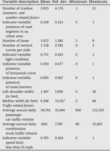
available for the present study include highway functional class, highway segment length, terrain category (i.e., level, rolling, and mountainous), type of gradient (i.e., vertical curve, angle point or gap), direction of grade, percentage of grade, type of access control, shoulder width and type, median width and type, lane type and number, pavement surface condition, and light condition (i.e., dawn, dusk, daylight, dark with road lighted, dark with street lights off, and dark with no street lights). The traffic flow features include intersection control type, posted speed limit, average annual daily passenger traffic volume, percentage of combination truck traffic, and average annual daily combination truck traffic volume. The crash data include crash severity (i.e., fatality, injury, and property damage only), crash category (has over twenty de-scriptions including rear end collision), and number of crashes on a highway segment. The remaining variable groups include weather, and period of the year/month during the crash. But not all the variables were available for the duration of the analysis, which leads to the reduction of the highway seg-ments to 158. The descriptive statistics of the variables found to be statistically significant in the forthcoming modeling frameworks are presented inTable 1.
3.
Methodology
To analyze the impacts of the selected variables related to highway geometric, traffic flow, weather, and spatial features
Table 1eDescriptive statistics of selected variables.
Variable description Mean Std. dev. Minimum Maximum Number of crashes 3.815 4.176 1 51 Geometric- and weather-related factors Indicator variable: presence of road segment in an urban area 0.109 0.312 0 1 Number of lanes 3.472 1.382 2 8 Number of vertical
curves per mile
1.158 0.582 0 3 Indicator variable: light condition 0.751 0.432 0 1 Indicator variable: presence of horizontal curve 0.350 0.477 0 1 Indicator variable: presence of noise barriers 0.005 0.067 0 1
Left shoulder width (in feet)
1.397 2.830 0 30 Median width (in feet) 6.346 14.327 0 84 Traffic-related factors
Average annual daily passenger car traffic volume
34,743 33,444 856 212,333
Average annual daily combination truck traffic volume
1841 1799 60 31,850
Indicator variable: speed limit less than 55 mph
on crash frequency along a highway segment, a count data modeling technique is considered to be a suitable method, because highway crashes are nonnegative integers. There are a number of count data techniques that have been used in the literature including Poisson regression, negative binomial, and their derivatives (zero-inflated Poisson regression and zero-inflated negative binomial models) (Agbelie and Rosh-andeh, 2015; Mannering and Bhat, 2014).
In order to establish the basis of analysis, a simple Poisson framework for analyzing crash frequencies along a highway segment is shown as follow
Pð4iÞ ¼
expðtiÞti4i
4i!
(1) wherePð4iÞis the probability of a highway segmentihaving4i
crashes per year, ti is the specified Poisson parameter for
highway segment i. This specified Poisson parameter is
highwayi's expected crash frequencies,Eð4iÞ.
The Poisson regression specifies the crash frequency parametertias a function of explanatory variables using a
log-linear function is shown as
ti¼expðbXiÞ (2)
wherebis a vector of parameters that will be estimated,Xiis a
vector of explanatory variables.
If the Poisson model has to be selected, the data available
must have mean equal to the variance, such that
Eð4iÞ ¼Varð4iÞ. However, if this constraint is not met, the data
can be considered as either overdispersedðEð4iÞ<Varð4iÞÞor
underdispersedðEð4iÞ>Varð4iÞÞ.
Nonetheless, if the constraint is ignored during analysis, the standard errors of the estimated parameter vector will be inconsistent resulting in erroneous conclusions. To account for the likelihood of either overdispersion or underdispersion in the available data, a modified framework, a negative bino-mial model, is generally selected and it is derived by modi-fying Eq.(2)as
ti¼expðbXiþ3iÞ (3)
where expð3iÞis a gamma-distributed error term with mean 1
and variancem.
The extra term is included so that the variance can be allowed to be flexible and vary from the mean as Varð4iÞ ¼Eð4iÞ½1þmEð4iÞ ¼Eð4iÞ þmE2ð4iÞ.
The negative binomial probability density function can be written in this form as
Pð4iÞ ¼G½ð 1=mÞ þ4i Gð1=mÞ4i! 1=m ð1=mÞ þti 1=m t i ð1=mÞ þti 4i (4) whereGð$Þis a gamma function.
Asmapproaches zero, the Poisson regression becomes a
restrictive model of the negative binomial regression. There-fore, in cases where the dispersion factor,m is statistically significant, the selection of the negative binomial may be appropriate. Thus, the selection of either a Poisson model or a negative binomial model is dependent on the dispersion factor.
To account for the possible heterogeneity in the data which could vary from one highway segment to another, a
random-parameters model can be introduced. Besides, the individual parameters that can be estimated can be written as
bi¼bþai (5)
where ai is a randomly distributed term for each highway
segmenti.
There are a number of distributions that this term can take including Weibull, log-normal, Erlang, logistic, normal, etc. On the basis of Eq.(5), the crash frequency parametertibecomes tijai¼expðbXiþ3iÞ in the negative binomial with the
corresponding probabilities for Poisson or negative binomial nowPð4ijaiÞ. In this case, the log-likelihood function for the
random-parameters negative binomial is written as
LL¼X ci ln Z ai gðaiÞPð4ijaiÞdai (6)
wheregð$Þis the probability density function ofai.
In order to estimate the random-parameters model, the required numerical integration of the modeling using maximum likelihood estimation is computationally cumber-some (Agbelie, 2015). Therefore, a simulation-based maximum likelihood method is selected for the analysis, and the estimated parameters are those that maximize the simulated log-likelihood function while allowing for the
likelihood that the variance ai for highway segments is
statistically significant. In order to ensure efficient
distribution of draws for the numerical analysis, the simulation-based maximum likelihood was facilitated using Halton draws (Halton, 1960), which was demonstrated with be more superior compared with purely random draws (Greene, 2012).
To illustrate the relative magnitude between the response variable,ti (i.e., crash frequency), and the explanatory
vari-ables, on the basis of estimated parameters, marginal effect values are computed. For highway crash analysis, the mar-ginal effect values indicate the change in the frequency of crashes given a unit change in an explanatory variablex, and computed as the partial derivativevti=vx. Although marginal
effect values are computed for each highway segmenti, the averages over the highway segment population will be stated and discussed.
4.
Estimation results
In order to evaluate the impact of the explanatory variables on highway crash frequency, negative binomial and random-parameters negative binomial models are considered. The two modeling methods are used in the analysis due to over-dispersion in the data. The random-parameters model is estimated on the basis of a simulation-based maximum like-lihood. To estimate the model, a 200 Halton draws is consid-ered because this number of draws has been proven to produce consistent and accurate parameter estimates ( Agbe-lie and Roshandeh, 2015; Bhat, 2003), and the efficiency of Halton draws is also significant compared with random draws (Train, 2003). A number of distributions, including triangular, uniform, log-normal, and normal, are initially examined to facilitate the selection of the random-parameters negative
binomial density functional forms. However, the normal distribution provides the best fitting among distributions examined. In order to test whether an estimated parameter should be considered as randomly distributed or fixed, the standard deviation of the parameter density is examined. When the standard deviation of a parameter density is found to be statistically significant, the estimated parameter is considered randomly distributed across the population of
highway segments being considered. However, the
estimated parameter will be considered fixed, if the estimated standard deviation is not statistically significant. In the present paper, a 1% significance level is considered, thus, the critical value for a two-tailed test is 2.576.
The estimated results are presented inTable 2, and the marginal effects are presented in Table 3. The dispersion factors observed from both models are found to be statistically significant, suggesting a significant difference between the variance and the mean of the dependent variable. The dispersion factor for the random-parameters model is 22.456, and thet-statistics value of 12.169 is greater than the critical value for a two-tailed test of 2.576.
The random-parameters negative binomial results inTable 2show a significantly better log-likelihood at convergence and better overall fit with ther2improving from 0.18 in the fixed-parameters negative binomial model to 0.68 in the random-parameters model. In order to test which of the two models was statistically superior, a likelihood ratio test was
conducted. The equation of test statistics is
c2¼ 2½LLðb
FPÞ LLðbRPÞ, where LLðbFPÞis the log-likelihood at convergence of the fixed-parameters negative binomial model, LLðbRPÞ is the log-likelihood at convergence of the random-parameters negative binomial model (Greene, 2012). The statistic, c2, distributed with degrees of freedom equal to the difference in the numbers of estimated parameters between the random-parameters negative binomial model and the traditional fixed-parameters negative binomial model. The computedc2value is 32,378.4 with 7 degrees of freedom, giving a p-value closed to 0. The likelihood ratio test indicates that this study is more than 99.98% confidence that the random-parameters negative binomial model is
statistically superior to the fixed-parameters negative
binomial model. Besides, some of the estimated parameters for the fixed-parameters negative binomial model are found to be statistically insignificant at 1% significance level, while all the estimated parameters for the random-parameters negative binomial model are observed to be statistically significant at 1% significance level. On the basis of enhanced statistical significance and the better overall fit of the
random-parameters negative binomial model, the
impending discussions of the estimated parameters will be based on the results from the random-parameters negative binomial model.
The results of the random-parameters negative binomial model are presented in Table 2, and 12 variables produced
Table 2eNegative binomial and random-parameters negative binomial models for annual accident frequencies (all random parameters are normally distributed).
Variable description Negative binomial Random-parameters negative binomial
Estimated parameter t-statistic value p-value Estimated parameter
t-statistic value p-value Constant
(standard
deviation of parameter distribution)
0.521 7.260 0.000 0.574 (0.033) 11.305 (5.716) 0.000
Geometric- and weather-related factors Indicator variable: presence of
road segment in an urban area
0.261 3.314 0.009 0.199 3.780 0.000 Number of lanes (standard deviation
of parameter distribution)
0.051 5.401 0.000 0.042 (0.054) 6.048 (23.818) 0.000 Number of vertical curves per mile
(standard deviation of parameter distribution)
0.002 16.513 0.000 0.002 (0.002) 18.574 (27.479) 0.000 Indicator variable: light condition 0.070 4.716 0.000 0.052 4.117 0.000 Indicator variable: presence of horizontal curve 0.084 2.274 0.023 0.084 2.788 0.005 Indicator variable: presence of noise barriers 0.298 5.768 0.000 0.163 (0.517) 4.487 (85.927) 0.000 Left shoulder width (in feet) 0.027 7.803 0.000 0.022 8.469 0.000
Median width (in feet) 0.002 1.903 0.057 0.002 2.655 0.008
Traffic-related factors
Average annual daily passenger car traffic
volume (standard deviation of parameter distribution)
4.585104 16.702 0.000 3.436106
(3.527106)
14.790 (29.021) 0.000 Average annual daily combination truck traffic volume
(standard deviation of parameter distribution)
1.449104 1.935 0.053 0.002 (0.007) 1.980 (9.648) 0.047
Indicator variable: speed limit less than 55 mph (standard deviation of parameter distribution)
0.263 10.169 0.000 0.188 (0.169) 9.291 (52.516) 0.000 Dispersion parameter 0.465 44.448 0.000 22.456 12.169 0.000 Number of observations 158 Log-likelihood at zero LL(0) 32,090.77 Log-likelihood at convergence LL(b) 26,312.43 10,123.21 r2¼1LLðbÞ =LLð0Þ 0.18 0.68
statistically significant parameters, including the constant term. In Table 2, the numbers in parenthesis indicate that the estimated parameter varies significantly across highway segments, and the standard deviation of the parameter distribution is also shown under each parameter, and the corresponding t-statistics value. In order to appreciate the broad factors considered in the present study and for easy comprehension, the parameters are broadly divided into geometric- and weather-related factors (i.e., road segment in an urban area, number of lanes, number of vertical curves per mile, daylight condition, presence of horizontal curve, presence of noise barriers, left shoulder width, and median width), and traffic-related factors (i.e., average annual daily
passenger car traffic volume, average annual daily
combination truck traffic volume, and speed limit less than 55 mph).
Examination of the results show that a highway segment located in an urban area (population greater than 50,000 people) is more likely to have a decreased highway crash frequency compared with a highway segment outside an urban area. The presence of an urban area reduces highway crashes by a fixed rate of 0.604 crashes per year.
The number of lanes on a highway segment produces a normally distributed parameter that is positive for 78.16% of the highway segments and negative for 21.84% of the highway segments. A unit increase in the number of lanes will increase crash frequency by 0.127 for 78.16% of the highway segments, but decrease crash frequency for 21.84% of the highway segments.
The number of vertical curves per mile along a segment produces a normally distributed parameter that is positive for 84.13% of the highway segments and negative for 15.87% of the
highway segments. A unit increase in the number of vertical curves per mile along a highway segment would increase mean annual crash frequency by 0.006 for most of the highway segments, and this could be possibly due to the unfamiliarity of the alignment by road users resulting in the increase of crashes when they approach sections with more vertical curves. Nonetheless, the estimated parameter also decreased crash frequency for 15.87% of the highway segments.
The number of crashes occurring on light highways has a negative fixed parameter. Thus, the presence of light on a highway results in a 0.157 decrease in the average annual number of crashes. The result indicates that an increase in light condition would reduce crash frequency, and it could be likely due to the drivers being able to see, thus, drivers have adequate sight distances and can properly respond to changes on highway segments.
The presence of a horizontal curve along a highway segment is found to increase average annual crash frequency. The variable yielded a fixed positive parameter estimate, and a unit increase in the presence of horizontal curves along a highway segment would increase mean annual crash fre-quency by 0.254. This finding indicates the increased likeli-hood of crashes along highway segments with the presence of horizontal curves.
Noise barriers are primarily used to mitigate the frequency and intensity of sound transmitted to buildings due to prox-imity of buildings to highways. The presence of them on a highway segment produces a normally distributed parameter that is positive for 88.21% of the highway segments and negative for 11.79% of the highway segments. Besides, it would increase mean annual crash frequency by 0.492 for most of the highway segments. However, the presence of noise barriers also decreases crash frequency for 11.79% of the highway segments.
The effect of left shoulder width on a highway was inves-tigated. A unit increase in left shoulder width decreases mean annual crash frequency by 0.067. Besides, highway median width produced a fixed parameter and a unit increase in me-dian width would decrease annual number of crashes by 0.006 along highway segments. The result likely suggests that wider median serves as a buffer zone for exit, assuming there is potential for a crash.
All three traffic-related estimated parameters, including average annual daily passenger car traffic volume, average annual daily combination truck traffic volume, and speed limit less than 55 mph, produce normally distributed param-eters across highway segments. The number of passenger cars along a highway segment produced a normally distributed parameter and a unit increase in passenger car daily volume will increase crash frequency by 1.038103for 83.50% of the highway segments, and decrease the number of crashes per year for 16.50% of the segments. A unit increase in the number of combination trucks along a highway segment would decrease crash frequency by 0.007 for 61.25% of the highway segments, and increase the number of crashes per year for 38.75% of the segments. The effect of traffic volume is mixed. For passenger vehicles, an increase in their numbers increases crash frequencies, while for combination trucks, an increase in traffic volume decreases crash frequency. The results imply that increasing the number of passenger vehicles on the
Table 3eMarginal effects: negative binomial model vs. random-parameters negative binomial model for annual accident frequencies (all random parameters are normally distributed).
Variable description Negative
binomial marginal effects (NBME) RP negative binomial marginal effects (RPNBME) Geometric- and weather-related factors Indicator variable: presence of
road segment in an urban area
1.000 0.604 Number of lanes 0.195 0.127 Number of vertical curves per mile 0.008 0.006 Indicator variable: light condition 0.267 0.157 Indicator variable: presence
of horizontal curve
0.039 0.254 Indicator variable: presence
of noise barriers
1.139 0.492 Left shoulder width (in feet) 0.104 0.067 Median width (in feet) 0.008 0.006 Traffic-related factors
Average annual daily passenger car traffic volume
1.755103 1.038103
Average annual daily combination truck traffic volume
5.546104 0.007
Indicator variable: speed limit less than 55 mph
highway increases the number of crashes and the result could be due to the increased interaction of motorists on a highway segment as the traffic volume increases. The increased interaction of passenger vehicles could be likely due to lower speeds on these segments. The speed limit indicator variable result shows that, highway segments with speed limits lower than 55 mph are found to have 0.568 (Table 3) more crashes per year for 86.7% of the highway segments, but less crashes for the remaining 13.3% of the highway segments.
5.
Conclusions
The present study conducts an empirical highway segment crash frequency analysis on the basis of two models, negative binomial and random-parameters negative binomial. The data used for the analysis are obtained from police-reported highway segment crash data related to highway geometric, weather, spatial features and traffic conditions from Wash-ington State. Using a total of 158 highway segments from 2008 to 2011, with 11,168 crashes, the results from both models were presented, discussed, and compared.
Out of a total of 12 final variables for the models, including the constant term, 7 variables (i.e., constant term, number of lanes, number of vertical curves per mile, presence of noise barriers, average annual daily passenger car traffic volume, average annual daily combination truck traffic volume, and speed limit less than 55 mph) produce normally distributed parameters across highway segments, while the remaining 5 produces fixed parameters.
The random-parameters negative binomial analysis is found to adequately account for unobserved heterogeneity in crash frequency across highway segments compared with the traditional negative binomial model. Out of the two models (negative binomial and random-parameters negative bino-mial), the random-parameters negative binomial model is found to be a superior model due to a relatively higher log-likelihood at convergence, better overall model fit, r2, and improved statistical significance of the estimated parameters. Besides, the random-parameters model adequately accounts for the variation of parameters across highway segments to ensure consistent parameter estimates. In practice, the results of the random-parameters model can be used to enhance the understanding of the significant variables that impact highway segment crash frequency. Overall, the results indicate that the use of the random-parameters negative binomial model is able to better capture the statistical significance of most of the pa-rameters compared with the fixed negative binomial model, and also explains the variation in the data adequately compared with the traditional negative binomial model.
Acknowledgments
The author is grateful to Highway Safety Information System for the assistance in providing the dataset. The opinions expressed in the present paper are, however, solely those of the author.
r e f e r e n c e s
Agbelie, B.R.D.K., 2014. An empirical analysis of three econometric frameworks for evaluating economic impacts of transportation infrastructure expenditures across countries. Transportation Policy 35, 304e310.
Agbelie, B.R.D.K., 2015. Random-parameters analysis of energy consumption and economic output on carbon dioxide emissions. Energy Systems. http://dx.doi.org/10.1007/s12667-015-0181-5.
Agbelie, B.R.D.K., 2016. Random-parameters analysis of highway characteristics on crash frequency and injury severity. Journal of Traffic and Transportation Engineering (English Edition) 3 (3), 236e242.
Agbelie, B.R.D.K., Roshandeh, A.M., 2015. Safety impacts of signal-related characteristics at urban signalized intersections. Journal of Transportation Safety&Security 7 (3), 199e207.
Bhat, C.R., 2001. Quasi-random maximum simulated likelihood estimation of the mixed multinomial logit model. Transportation Research Part B: Methodological 35 (7), 677e693.
Bhat, C.R., 2003. Simulation estimation of mixed discrete choice models using randomized and scrambled Halton sequences. Transportation Research Part B: Methodological 37 (9), 837e855.
Cameron, A., Trivedi, P., 1986. Econometric models based on count data: comparisons and applications of some estimators and tests. Journal of Applied Econometrics 1 (1), 29e53.
Greene, W., 2012. Econometric Analysis, seventh ed. Prentice-Hall, Boston.
Gustavsson, J., Svensson, A., 1976. A Poisson regression model applied to classes of road accidents with small frequencies. Scandinavian Journal of Statistics 3 (2), 49e60.
Halton, J., 1960. On the efficiency of certain quasi-random sequences of points in evaluating multi-dimensional integrals. Numerische Mathematik 2 (1), 84e90.
Lord, D., Guikema, S.D., Geedipally, S.R., 2008. Application of the ConwayeMaxwellePoisson generalized linear model for analyzing motor vehicle crashes. Accident Analysis &
Prevention 40 (3), 1123e1134.
Mannering, F., Bhat, C.R., 2014. Analytic methods in accident research: methodological frontier and future directions. Analytic Methods in Accident Research 1, 1e22.
McFadden, D., Train, K., 2000. Mixed MNL models for discrete response. Journal of Applied Econometrics 15 (5), 447e470.
Milton, J., Shankar, V., Mannering, F., 2008. Highway accident severities and the mixed logit model: an exploratory empirical analysis. Accident Analysis & Prevention 40 (1), 260e266.
Savolainen, P.T., Tarko, A.P., 2005. Safety impacts at intersections on curved segments. Transportation Research Record 1908, 130e140.
Train, K., 2003. Discrete Choice Methods with Simulation. Cambridge University Press, Cambridge.
Bismark R. D. K. Agbelieis currently a post-doctoral researcher and a visiting instructor at the Lyles School of Civil Engineering at Purdue University, West Lafayette. His research interests include transportation systems analysis; transportation infrastruc-ture economics, finance, and management; transportation safety, policy analysis, and costs analysis of engineering systems.