UW Biostatistics Working Paper Series
6-22-2016
A Powerful Statistical Framework for
Generalization Testing in GWAS, with Application
to the HCHS/SOL
Tamar Sofer
University of Washington, [email protected]
Ruth Heller
Tel-Aviv University, [email protected]
Marina Bogomolov
Technion-Israel Institute of Technology, [email protected]
Christy L. Avery
University of North Carolina at Chapel Hill, [email protected]
Mariaelisa Graff
University of N Carolina, Chapel Hill, [email protected] See next page for additional authors
Suggested Citation
Sofer, Tamar; Heller, Ruth; Bogomolov, Marina; Avery, Christy L.; Graff, Mariaelisa; North, Kari E.; Reiner, Alex; Thornton, Timothy A.; Rice, Kenneth; Benjamini, Yoav; Laurie, Cathy C.; and Kerr, Kathleen F., "A Powerful Statistical Framework for Generalization
Authors
Tamar Sofer, Ruth Heller, Marina Bogomolov, Christy L. Avery, Mariaelisa Graff, Kari E. North, Alex Reiner, Timothy A. Thornton, Kenneth Rice, Yoav Benjamini, Cathy C. Laurie, and Kathleen F. Kerr
A Powerful Statistical Framework for Generalization Testing
in GWAS, with Application to the HCHS/SOL
Tamar Sofer,1⇤ Ruth Heller,2 Marina Bogomolov,3 Christy L. Avery,4
Mariaelisa Gra↵,4 Kari E. North,4 Alex P. Reiner,5 Timothy A. Thornton,1
Kenneth Rice,1 Yoav Benjamini,1 Cathy C. Laurie,1 and Kathleen F. Kerr1 1Department of Biostatistics, University of Washington, Seattle, WA 98105, USA
2Department of Statistics and Operations Research, Tel-Aviv University, Tel-Aviv, 6997801, Israel
3Faculty of Industrial Engineering and Management, Technion-Israel Institute of Technology, Haifa 3200003, Israel 4Department of Epidemiology, University of North Carolina, Chapel Hill, NC 27514, USA
5Division of Public Health Sciences, Fred Hutchinson Cancer Research Center, Seattle, WA 98195, USA
Abstract
In GWAS, “generalization” is the replication of genotype-phenotype association in a population with di↵erent ancestry than the population in which it was first identi-fied. The standard for reporting findings from a GWAS requires a two-stage design, in which discovered associations are replicated in an independent follow-up study. Current practices for declaring generalizations rely on testing associations while controlling the Family Wise Error Rate (FWER) in the discovery study, then separately controlling error measures in the follow-up study. While this approach limits false generaliza-tions, we show that it does not guarantee control over the FWER or False Discovery Rate (FDR) of the generalization null hypotheses. In addition, it fails to leverage the two-stage design to increase power for detecting generalized associations. We develop a formal statistical framework for quantifying the evidence of generalization that ac-counts for the (in)consistency between the directions of associations in the discovery and follow-up studies. We develop the directional generalization FWER (FWERg) and FDR (FDRg) controlling r-values, which are used to declare associations as general-ized. This framework extends to generalization testing when applied to a published list of SNP-trait associations. We show that our framework accommodates various SNP selection rules for generalization testing based onp-values in the discovery study, and still control FWERg or FDRg. A key finding is that it is often beneficial to use a more lenientp-value threshold then the genome-wide significance threshold. For instance, in a GWAS of Total Cholesterol (TC) in the Hispanic Community Health Study/Study of Latinos (HCHS/SOL), when testing all SNPs withp-values<5⇥10 8 (15 genomic
regions) for generalization in a large GWAS of whites, we generalized SNPs from 15 re-gions. But when testing all SNPs withp-values<6.6⇥10 5(89 regions), we generalized SNPs from 27 regions.
Introduction
When presenting results from genome-wide association studies (GWAS), current standards require a “two-stage design” in which possible discoveries in the first stage are replicated in an independent study (Cohen, 1999). ‘Generalization’ is the replication of a genotype-phenotype association in a population with di↵erent ancestry (or other characteristics) than the population in which it was first identified. Increasingly, generalization testing is performed as part of this two-stage design, primarily because GWAS is expanding into populations of diverse ancestry. First, with non-white discovery populations, there tend to be fewer similar studies available, so only generalization and not replication is feasi-ble. Second, if the discovery study population is admixed (e.g. Hispanics/Latinos), it is customary to seek generalization in some of its parental populations.
Interestingly, even though the current standard for GWAS mandates replication, er-ror controlling multiple testing adjustment procedures are often applied separately in the discovery and follow-up stages, without employing a replication- or generalization- based statistical framework. Bogomolov and Heller (2013) have shown that such approaches do not guarantee control over false generalization claims. Let the generalization null hypoth-esis state that a SNP is not associated with the trait in the discovery population, the follow-up population or both; and this null is rejected if evidence of association exists for both populations. Define generalization testing as any multiple testing adjustment
pro-cedure that controls measures of generalization error such as the Family-Wise Error Rate (FWERg) or the False Discovery Rate (FDRg). In this paper, we propose methods to test
the generalization null hypotheses in GWAS, by expanding and adapting recent statistical methods developed for replication.
Bogomolov and Heller (2013) considered replication testing using discovery and follow-up studies, and developed multiple testing procedures with protection against erroneous replicability claims by controlling the FWERg or the FDRg. They showed that one must
account for multiple testing in both the discovery and the follow-up studies to avoid a high number of erroneous replicability claims. Heller et al. (2014) suggested improvements to these procedures when used for GWAS, and developedr-values to quantify the evidence for replication while controlling FWERg or FDRg in GWAS. However, the r-values in Heller
et al. (2014) do not account for the direction of the observed association. In this work we extend the r-values approach to incorporate the direction of observed associations. This acknowledges that we do not want to claim that an association generalizes if the direction of e↵ect is di↵erent in the two populations. Our procedure performs directional control by using one-sided p-values to compute directional r-values at the generalization testing stage, despite using two-sided tests in the discovery stage. This makes our procedure more powerful than the procedure of Heller et al. (2014) for discovering associations with the same direction in both studies. We perform extensive simulations to study fixed and data-adaptive rules for selecting SNPs based on their p-values in the discovery study, and compare multiple-testing adjustment procedures in combination with these selection rules.
Materials and Methods
The generalization multiple testing framework
Expanding on the formal framework for replication of Heller et al. (2014), here we describe the generalization null hypothesis, propose a multiple testing adjustment procedure for generalization analysis, and contrast it with procedures currently used for single-stage studies.
Generalization versus discovery null hypotheses
There are two crucial di↵erences between testing SNPs in a single-stage versus two-stage study design. In a single-stage design, all eligible SNPs in a single study are tested (after quality control filters). In contrast, in a two-stage design (1) the set of SNPs considered for generalization testing is based on results from the discovery study, and (2) tests of the null hypotheses are based on association analysis results from both the discovery and the generalization studies. Thus, suppose that m SNPs are tested in the discovery study. In a single-stage design, the discovery null is rejected for all significant associations in this study. However, in a two-stage design, the generalization null hypothesis is rejected when a SNP is associated with the trait in the generalization study as well, and the directions of association are the same.
Measures of false generalization
In multiple testing, there are two common measures of error: the FWER, and the FDR. In a single-stage GWAS, FWER is the probability of rejecting at least one null hypothesis
corresponding to a SNP not associated with the trait. FDR is the expected proportion of false null rejections out of all rejections, i.e. the expected proportion of falsely detected SNPs out of all those reported as associated with the trait. We describe the FWER and FDR for generalization testing.
Define the left-sided (right-sided) alternative as the scenario in which a given SNP allele is negatively (positively) associated with the trait in a given study (either discovery or follow-up). Let Hij = 8 > > > > > < > > > > > :
1 if the right-sided alternative is true for SNP j in populationi
0 if the null hypothesis of no association is true for SNP j in populationi 1 if the left-sided alternative is true for SNP j in populationi
Let Hj = {h= (h1j, h2j) :hij 2{ 1,0,1}} be the set of 9 possible configurations of the
vectorHj = (H1j, H2j) for two-sided alternatives for SNPj. The set of possible
configu-rations is depicted in Figure 1. The generalization null hypothesis for SNP j is true ifHj
belongs to the set H0 = {( 1,1),( 1,0),(1, 1),(1,0), (0,0),(0, 1),(0,1)}. A SNP for
which the generalization null is false hasHj 2HA={(1,1),( 1, 1)}.
For a SNPj, denote byRR
j and RLj the indicators of whether a generalization null
re-jection (“generalization claim”) is made in the right or left direction, respectively. Suppose thatR generalization claims are made by an analysis. The number of true generalization claims is S= X {j:Hj=(1,1)} RRj + X {j:Hj=( 1, 1)} RLj,
The directional generalization (and replication) FWER and FDR are given by: FWERg = P r(R S >0), FDRg = E ✓ R S max(R,1) ◆ .
Controlling for false generalizations
Heller et al. (2014) proposed r-values for testing associations in both the discovery and generalization (or replication) studies. Notably, Heller et al. (2014)’s procedure is not con-cerned with directional consistency. We now extend the procedure proposed by Heller et al. (2014) to the directionalr-values framework and procedure for directional control in gen-eralization testing. Following the definitions given below, the procedures are provided, and the proofs that these procedures control FDRg/FWERg are relegated to the supplemental
material.
Definition: The directional FDRg/FWERg r-value for a SNP is the lowest FDR/FWER
level at which we can say that the SNP association is generalized with the same direction of association in both the discovery and generalizing studies.
The directionalp-values: Denote the left- and right-sidedp-values for SNP associationj in studyi2{1,2}bypLij, pRij respectively. For continuous test statistics,pRij = 1 pLij. The p-values (p01j, p02j) corresponding to variant jused in generalization analysis are defined as:
p01j = 8 > < > : pL 1j ifpL1j < pR1j pR1j ifpL1j > pR1j p02j = 8 > < > : pL 2j ifpL1j < pR1j pR2j ifpL1j > pR1j.
Note that the one-sidedp-values from both studies are guided by the estimated direction of association in the discovery study, so that if the association of SNP j was in the nega-tive (posinega-tive) direction, then p01j <0.5 is the left (right) sided hypothesis p-value in the discovery study, andp02j is the left (right) sided hypothesisp-value in the follow-up study. Therefore, if the evidence towards association is in the same direction in both studies, both p01j, p02j <0.5, but if the estimated associations are in opposite directions in the two studies, thenp02j >0.5.
Data and parameters required for FDRg/FWERg r-values computation:
1. m, the number of SNPs examined in the discovery study.
2. R1, the set of SNPs selected for follow-up based on discovery study results. Let R1 =|R1|be their number.
3. The directionalp-values for the followed-up SNPs {(p01j, p02j) :j2R1}.
4. l002[0,1), the user-specified lower bound on the fraction of SNP associations, out of
them SNPs examined in the discovery study, that are null in both studies. Default value for a GWAS isl00= 0.8, following Heller et al. (2014).
5. c22(0,1), the emphasis given to the follow-up study (see Section Variations in Heller
et al. (2014)), default value isc2 = 0.5.
Computation of the FDRg/FWERg r-values
1. Defining functionsfF DR
(a) Computec1(x) = 1 l001(1c2c2x), the inverse weight function for thep-values from
the discovery study.
(b) For every SNPj2R1 compute the following e-values:
ej(x) = max ✓ m c1(x) p01j, R1 c2 p02j ◆ , j 2R1. (C) [FDR] LetfF DR i (x) = min{j:ej(x) ei(x),j2R1} ej(x)
rank[ej(x)], whererank[ej(x)] is the rank of thee-value for a SNPj2R1 (with maximum rank for ties).
(C) [FWER] LetfjF W ER(x) =ej(x).
2. The FDRg (FWERg) r-value for SNP i 2 R1 is the solution to fiF DR(ri) = ri
(fF W ER
i (ri) = ri) if a solution exists in (0,1), and 1 otherwise. The solution is
unique, see Lemma S1.1 in Heller et al. (2014).
The directional procedure for establishing generalization with FDRg/FWERg
control at level q.
1. Compute the FDRg/FWERg r-values.
2. Declare as generalized all SNPs with FDRg/FWERg r-value at mostq. Denote this
set of SNPs byR2.
3. If a SNP j 2R2 hasp01j = pL1j, then declare this SNP as having a generalized
left-sided alternative; If SNP j 2 R2 has p01j = pR1j, then declare the SNP as having a
Selection rules
In generalization analysis, SNP associations are first tested in the discovery study, and then a smaller subset of these SNPs is selected for testing in the follow-up study, accord-ing to a selection rule. The most well known selection rule is the one that selects SNPs with p-value< 5⇥10 8 in the discovery study. This selection rule originates in single-stage designs, in which one has to report significant findings in the discovery study while controlling the FWER, assuming that m = 106. We consider other selection rules for a generalization/replication-based study design where the null hypothesis is the generaliza-tion null hypothesis.
1. Selection rule 1, recommended by Heller et al. (2014) for FDRg control. Apply
the FDR controlling BH procedure (Benjamini and Hochberg, 1995) on allp-values from the discovery study to obtain BH-adjusted p-values. Choose all SNPs with BH-adjustedp-valuet, where
t = c1(q)⇤q, with (1)
c1(x) =
0.5 1 l00(1 0.5x)
.
Useq= 0.05 to control FDRg at the 0.05 level. The rationale behind selection rule 1
is that every SNP with BH-adjusted discoveryp-value larger thanthas no chance of generalizing. Heller et al. (2014) applied this selection rule in settings where either both discovery and replication used two-sided p-values, or both used one-sided p -values with pre-determined direction. We can also apply it on one-sided p-values
2. Selection rule 2, recommended by Heller et al. (2014) for FWERg control. This rule
selects all SNPs with discoveryp-valuet0, where
t0=c1(q)⇥q/m. (2)
As in selection rule 1, SNPs withp-value> t0 have no chance of generalizing using the FWERg controlling procedure and selecting them may only reduce power. Again, we
can apply this selection rule on the one-sidedp-values used for generalization testing. Note that selection rule 1 is data adaptive, and depends on the distribution of signals in the discovery study. Selection rule 2 is a fixed threshold rule. In selection rule 2, if l00 = 0.8, q = 0.05, and m = 106, we get t0 = 1.14⇥10 7. When one-sided p-values are
used for generalization testing, the original two-sided p-values passing this threshold are
2.28⇥10 7.
Linkage Disequilibrium (LD)
GWAS datasets may potentially contain tens of millions of genotyped and imputed SNPs. Many of these SNPs are in linkage disequilibrium; that is, allelic variation within one SNP is correlated with allelic variation in another SNP. Often, when a discovery study association is detected, the locus may contain tens of correlated SNPs with low p-value. All of the significant SNPs may be tagging the same underlying causal genetic variant, or there may be multiple causal variants (referred to as “allelic heterogeneity”). Usually, the SNP with lowest p-value among the set of correlated SNPs is identified as the “lead”, or “sentinel”, SNP and is the one reported. There are two important issues in generalization testing of
1. When testing all associated SNPs (compared to a single SNP from any set of SNPs in LD), the multiple testing burden is larger than when testing only independent SNPs. In applying FWER-type control, this issue is sometimes handled by calculating the e↵ective number of independent SNPs, and using this number in applying a Bonferroni correction. In contrast, this is not a problem for FDR control, which is concerned with fractions of false positives.
2. The pattern of LD usually di↵er between two di↵erent populations, and consequently di↵erent SNPs may best tag the underlying causal genetic variation.
Therefore, if appropriate information is available (e.g. the LD matrix of the SNPs in the generalization study), we recommend following-up on all SNPs passing the appropriate p-value threshold and using the e↵ective number of tests instead of the actual number of selected SNPs in computingr-values.
Simulation studies: discovery and generalization GWAS
In this section, we examine the performance of our methods when the discovery study hypotheses tests are two-sided. In particular, we examine the gain in power from using one-sided p-values guided by the evidence in the discovery study, compared to applying the two-sided p-values in the procedure suggested by Heller et al. (2014). We also assess the impact of using di↵erent selection rules on generalization power.
In the simulation study described below, we directly simulated test statistics for two studies. This approach allowed us to conduct a large number of simulations, and study
low minor allele counts), where inflation means that thep-values distribution is left-skewed rather than uniform under the null. First, test statistics were calculated in the discovery study, and then SNPs were selected for generalization testing based on several selection rules. We used selection rules 1 (for FDRg control) and 2 (for FWERg control), applied
on both one- and two-sidedp-values. We also used the selection rules that take all SNPs withp-values<1⇥10 6,1⇥10 7, and<5⇥10 8 in the discovery study.
In an additional simulation study, we investigated GWAS of cohorts designed to mimic realistic data sets with di↵erences in LD structure and MAFs between the discovery and the generalization cohort (supplemental material) in a smaller number of simulations. There, we also compared generalization testing of all SNPs satisfying the selection rule with the testing of only the lead SNPs from each of the detected loci.
Simulating test statistics with null inflation
In each of 1,000 repetitions of the simulations, we sampled a million independent test statistics for both the discovery and the follow-up studies. Of these SNPs, 100 were causal in the discovery study and 100 were causal in the follow-up study. 50 of the causal SNPs overlapped between the studies. We considered two common generalization scenarios. In the first setting the discovery study had relatively low power, and the follow-up study has high power. For instance, this happens when discovery is performed in the HCHS/SOL, and follow-up is pursued in a large meta-analysis GWAS in individuals of Europeans ancestry. In the second setting the discovery study had high power, and the follow-up study had low power. This happens when investigators in the HCHS/SOL study the generalization
to Hispanics/Latinos of associations that were formerly reported in large meta-analyses of whites.
In both settings, the test statistics corresponding to causal SNPs in the discovery study 1 were sampled, in each simulation, asz1,j ⇠N(u1j,1) where u1j is a realization of
a random variable sampled from unif(ul, uh) distribution. When the discovery study had
lower power we setul = 4, uh= 5. Corresponding two-sided p-values had a medianp-value
of 7⇥10 6, with an inter-quartile range of [2⇥10 7,1⇥10 4]. When the discovery study
had high power we set ul = 5, uh = 6. Corresponding two-sidedp-values had a median p
-value of 4⇥10 8, with an inter-quartile range of [5⇥10 10,2⇥10 6]. The 100 test statistics corresponding to the causal SNPs in study 2 were similarly sampled as z2,j ⇠ N(u2j,1)
whereu2j ⇠unif(5,6) when the follow-up study had high power, andu2j ⇠unif(3,4) when
the follow-up study had low power; the latter had corresponding two-sidedp-values with a medianp-value of 5⇥10 4 and an inter-quartile range of [3⇥10 5,5⇥10 3]. Finally, we generated inflation via a simple procedure in which the test statistics corresponding to non-causal (null) SNPs, in both the discovery and the generalizing cohorts, were independently sampled from a Normal distribution with mean of zero and variance of 1.21, corresponding to gc = 1.21 (Devlin and Roeder, 1999).
We studied additional simulation settings: a 90% overlap of the causal SNPs between the two populations, a larger number of causal SNPs (1,000 and 10,000), and a discovery study with u1j ⇠unif(4,5), corresponding to two-sided p-values having a median p-value
of 7⇥10 6, with an inter-quartile range of [2⇥10 7,1⇥10 4], and follow-up study with u2j ⇠ unif(3,4). Overall, our simulations covered many plausible scenarios of the power
of the discovery and follow-up studies (high, medium, and low discovery power, and high and low follow-up study power), and reasonable assumptions on the overlap between the genetic component of the two populations, and on the number of SNPs associated with the trait. Finally, we also studied the e↵ect of setting l00 to 0.9,0.95.
The HCHS/SOL
The HCHS/SOL (LaVange et al., 2010; Sorlie et al., 2010), is a community based cohort study, following self-identified Hispanic individuals from four field centers (Chicago, IL; Miami, FL; Bronx, NY; and San Diego, CA). Individuals were sampled via a two-stage sampling scheme, in which households were randomly sampled from sampled block groups. Almost 13,000 study participants consented for genotyping. This study was approved by the institutional review boards at each field center, where all subjects gave written informed consent.
Genotyping, imputation and quality control
Blood samples from HCHS/SOL individuals were genotyped on a custom array consisting of Illumina Omni 2.5M content plus⇠150,000 custom markers selected to include ancestry-informative markers, variants characteristic of Amerindian populations, known GWAS hits and other candidate gene polymorphisms. Quality control was similar to the procedure de-scribed in Laurie et al. (2010), and included checks for sample identity, batch e↵ects, miss-ing call rate, chromosomal anomalies (Laurie et al., 2012), deviation from Hardy-Weinberg equilibrium, Mendelian errors, and duplicate sample discordance. 12,803 samples passed
quality control, and 2,232,944 SNPs passed quality filters. Pairwise kinship coefficients and principal components reflecting ancestry were estimated in an iterative procedure which accounts for admixture (Conomos, 2014; Conomos et al., 2016). Genome-wide imputation was done using the 1000 Genomes Project phase 1 reference panel.1000 Genomes Project Consortium (2012) Genotypes were first pre-phased with SHAPEIT2 (Delaneau et al., 2013) (v2.r644) and then imputed with IMPUTE2 (Howie et al., 2009) (v2.3.0).
Identifying SNP-TC associations in the HCHS/SOL
To study our proposed methods for identifying SNP-trait associations, we performed a GWAS of TC in the HCHS/SOL followed by generalization testing using publicly avail-able GWAS results. Our goal was to demonstrate that by using selection rules that are geared towards a two-stage study design, we can identify more generalized associations of independent loci, compared to selection rules that are based on a single-stage design.
The analysis was adjusted for sex, age, 5 principal components to control for confound-ing bias due to ancestry, and study design variables (e.g. study center, samplconfound-ing weights). Analysis was performed using linear mixed e↵ect models, with random e↵ects correspond-ing to block groups, households, and kinship. As advocated by Kraft et al. (2009), the HCHS/SOL analyses were matched to the published analyses, so that the same trait trans-formation was used in both analyses. Thus, we first regressed TC values on covariates, and then applied a rank-based inverse normal transformation on the residuals. We then used the transformed residuals as the trait in the association testing.
Con-sortium (GLGC) TC GWAS (Willer et al., 2013), conducted in a large meta-analysis of multiple cohorts of European ancestry comprising of over 180,000 individuals, to compare multiple generalization analyses of TC. First, we considered generalization geared towards establishing new associations, in which we perform a GWAS in the HCHS/SOL as a dis-covery stage, with generalizations to the independent GLGC data set. Second, we consider generalization with the goal of testing whether previously established associations extend to the HCHS/SOL. For this, we selected SNPs published by Teslovich et al. (2010) and Willer et al. (2013) to generalize to the HCHS/SOL.
As mentioned previously, we expect multiple SNPs from each detected locus to be associated with TC, due to LD. Therefore, we define a locus as the region of size 1Mb around a SNP. We tested all SNPs satisfying the selection rule criterion, even if they were in LD with each other. However, we report generalization results both in terms of SNP associations, and by loci: after generalization testing, we identified the first locus by taking the SNP with smallest discovery p-value (lead discovery SNP) to represent it. We then “removed” all SNPs in its vicinity, and continued to select other SNPs in a similar manner. A locus with any SNP that generalized is declared a generalized locus.
Results
Simulations
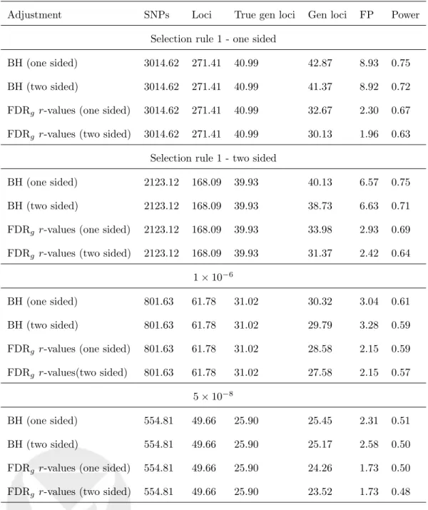
Tables 1 and 2 provide the simulation results when the discovery power was low and the follow-up study had high power, when the goal was to control FDRg and FWERg,
respectively. Tables 3 and 4 provide similar results for the setting where the discovery study power was high and the follow-up study had low power. In all tables we omitted the results for the selection rules that selected SNPs for follow-up based on discovery two-sided p-value10 7, as this resulted in “intermediate” results in terms of power between selection rules of higher and lower p-value thresholds, and is less beneficial than other selection rules.
For each selection rule, the characteristics of the selected SNP sets and generalization tests are provided, averaged across the iterations of simulations. The latter are provided in terms of estimated power, calculated as the average proportion of generalized SNPs, out of all generalizable SNPs in the simulation, false positives (FP) as the average number of generalizations of SNPs that are not in fact generalizable. In addition, when the selection rules and multiple testing adjustment methods were aimed at FDRg control (Tables 1 and
3), we also provide false discovery proportion (FDPg), which is the average proportion of
false positives out of all generalized SNPs, and estimates FDRg, and the standard deviation
of the false discovery proportion across all the simulations, SD(FDPg). When the selection
rules and multiple testing adjustment methods were aimed at FWERg control (Tables 2
and 4), we provide the estimated FWERg, as the proportion of simulations having at least
one false positive generalization, i.e. the mean of I[V >0], the indicator function of having at least one false generalization, i.e. V = R S >0, and also SD(I[V >0]). The standard
errors of all measures are also provided.
As expected throughout, the higher the p-value threshold implied by the selection rule, the larger the number of selected SNPs, and the larger the number of true generalizable
SNPs selected. As expected by chance, 50% of the non-generalizable candidate SNPs have di↵erent direction of estimated e↵ects in the two studies, so the one-sided p-values from the generalization study for these SNPs are higher than 0.5. Therefore, it is not surprising to see fewer false positive generalizations under directional control (using one-sided p -values). In both simulation settings and under both FDRgand FWERgcontrol, directional
control also had higher generalization power compared to using two-sided p-values, with less di↵erence when the selection rule had very lowp-values, or in other words, when fewer SNPs were under the null. In the settings in which the discovery study had high discovery power there was consequently higher generalization power, but also slightly higher error rates. Importantly, both FDRg and FWERg r-values always protected their target error
measures.
FDRg control: Focusing on directional FDRg r-values, selection rule 1 applied with
either one- or two-sided p-values was most powerful in the low discovery power setting, and selection rule 1 applied on two-sidedp-values was most powerful in the high discovery power setting. Generalization testing using BH on the follow-up study alone did not control FDRg when selection rule 1 was applied on one-sided p-values, and it also did
not control FDRg when applied on two-sided p-values. In lower p-value thresholds, when
a high proportion of the tested SNPs were under the alternative, FDRg was controlled
when BH was used on the follow-up study alone. Since the r-values approach is slightly more stringent than the BH on the follow-up approach, FDRg r-values are expected to be
somewhat less powerful. The di↵erence in power is small when the follow-up SNPs were highly significant. More specifically, the power is identical when the discovery power is low
and the selection rule is discoveryp-value10 6 or5⇥10 8, and the power di↵ered by only 0.03 for the same selection rules, when the discovery power is high.
FWERg control: Selection rule 2 applied on one-sided p-values was the most powerful
selection rule in both settings. Generalization testing using Bonferroni correction on the follow-up study alone never controlled FWERg, though error rates were slightly improved
by using one-sidedp-values.
Finally, additional simulations (results unreported) revealed the same pattern of results, overall suggesting that selection rule 1 applied on two-sided p-values is the most powerful for FDRgcontrol, and selection rule 2 applied on one-sidedp-values is the most powerful for
FWERg control. Settingl00 to higher values{0.9,0.95}had almost no e↵ect on the results
when selection rules with two-side discoveryp-values10 6 (or lower) were used, and had mixed e↵ects on power when selection rule 1 was used (beneficial in the low discovery power setting, but less powerful in the high discovery power setting).
The HCHS/SOL TC GWAS
HCHS/SOL as the primary discovery study in a two-stage design
We performed a GWAS of TC in the HCHS/SOL, to establish generalized SNP-TC asso-ciations. We test using both FDRg and FWERg controlling r-values, and compare them
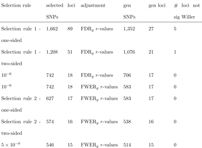
in combination with di↵erent selection rules. In Table 5, for each combination of selection rule and multiple testing adjustment method, we report the number of SNPs followed-up that are available in both the HCHS/SOL and the GLGC TC GWAS, the number of loci they correspond to, the number of generalized SNPs and generalized loci, and the number
of loci with none of the SNPs havingp-value<5⇥10 8 in Willer et al. (2013)’s GWAS. As expected, the number of SNPs selected for follow-up increased as thep-value thresh-old became higher; usually, the number of generalized loci increased as well. When the selection rule was all SNPs withp-value<5⇥10 8, the followed-up SNPs corresponded to 15 loci, all of which generalized under FWERg (and FDRg) control. For FWERg control,
the number of generalized loci was the same, and maximal (17 loci), with selection rule 2 (on one-sided p-values) and p-value< 10 6. This is consistent with the rationale behind
selection rule 2, because SNPs with HCHS/SOL two-sidedp-value>2.28⇥10 7 cannot be generalized under FWERg control.
In the FDRg-controlling analysis applied on SNPs satisfying selection rule 1 on
two-sidedp-values, 21 loci generalized. These included a single generalized locus that would not be reported in either the HCHS/SOL or the GLGC GWAS alone. The lead SNP, rs870992 on chromosome 5, had r-value= 0.008, HCHS/SOL p-value= 2⇥10 5, and GLGC p -value= 5.2⇥10 5. This SNP was formerly associated with concentration of liver enzymes in plasma in a GWAS(Chambers et al., 2011). In the FDRg-controlling analysis applied
on SNPs satisfying selection rule 1 with one-sided p-values, there were 22 loci with strong evidence of association in the GLGC GWAS (SNPs with p-values<5⇥10 8), and 5 loci
generalized that would not been detected in the HCHS/SOL or GLGC GWAS alone. One of them was the locus that includes rs870992. Another SNP, rs2072781 in chromosome 6, hadr-value= 0.009 (HCHS/SOLp-value= 2.1⇥10 5, GLGCp-value= 1⇥10 4). This SNP is in the MYLIP gene, formerly associated with high TC in Mexicans (Weissglas-Volkov et al., 2011). Three additional loci had relatively higher p-values in the GLGC GWAS
(0.007-0.05) andr-values in the range 0.01-0.05. The five loci are reported in Table S9 in the supplemental material.
In all analyses, there was a generalized locus in which the HCHS/SOL lead SNP did not generalize, as it had p-value= 0.92 in Willer et al. (2013), but a di↵erent SNP in the same locus hadp-value= 1.4⇥10 46in Willer et al. (2013) and generalized. This supports a strategy that analyzes all SNPs, rather than an LD-pruned set.
Generalizing previously reported TC-SNP associations
There are 74 SNPs previously reported as associated with TC withp-values5⇥10 8 and
are available for generalization testing in the HCHS/SOL data set. Teslovich et al. (2010), in a meta-analysis of more than 100,000 individuals, reported 51 SNPs, that were later replicated in Willer et al.,Willer et al. (2013) which further meta-analyzed their association testing results with additional results from the GLGC study. Willer et al. (2013) reported an additional set of 23 SNPs (that were not meta-analyzed with Teslovich et al.’sTeslovich et al. (2010) results). Therefore, we performed two generalization analyses: one for the 51 SNPs that were replicated and had meta-analysis results combining the two studies, and one for the set of 23 SNPs reported only in Willer et al.Willer et al. (2013) In this analysis, 33 of the formerly replicated SNPs generalized to the HCHS/SOL, while none of the SNPs that were only reported in Willer et al. (2013) generalized. This is likely due to their low e↵ect sizes.
In the supplemental material, we provide an additional analysis in which we follow-up for generalization testing all SNPs withp-value<10 6 in the GLGC GWAS, without any
SNP pruning. This analysis generalized 9 more loci than the analysis that tested only the published lead SNPs.
Discussion
In this work, we propose to leverage two-stage design to increase generalization power in GWAS. We show that by using a multiple testing adjustment framework tailored to the two-stage study design we can combine testing results from the discovery and follow-up studies to increase power with essentially no increase in the rate of false positive findings. We introduce procedures for calculating directional FDRg and FWERgr-values, computed
based on one-sidedp-values. We prove thatr-values control their directional error measures when there is no genomic inflation, and show via simulation that errors are controlled in the presence of inflation. These procedures are, by construction, more powerful than those based on two-sided p-values when the direction of association is consistent between discovery and follow-up populations. We studied SNP selection rules that are geared towards generalization-based designs, and found in simulation studies that by choosing SNPs for generalization testing based on p-values less conservative than the genome-wide significance threshold, e.g. selection rules 1 and 2 for FDRg control and FWERg control,
respectively, we are able to generalize more SNPs while controlling the desired error rate. Finally, we demonstrated our procedure on a GWAS of TC in the HCHS/SOL. First, we consider the scenario in which HCHS/SOL is a discovery study and generalization is required for reporting a significant finding. Second, we considered the scenario in which there are established SNP-trait associations that we want to generalize to the HCHS/SOL.
An approach that was promoted in the past to increase power in a two-stage design was to perform a joint analysis of the two studies via meta-analysis (Skol et al., 2006). However, this approach does not test the generalization null hypothesis, and an associ-ation may appear significant even if it exists only in one populassoci-ation. In contrast, our approach is focused in generalization testing; generalizations makes stronger statements on the underlying similarity in genetic associations between populations.
We provide practical recommendations based on our results. First, in terms of selection rules, we recommend selection rule 2 for FWERg control at the↵level, which selects SNPs
with two-sided discovery p-value< 2.28⇥10 7 for ↵ = 0.05. For FDRg control at the
↵ = 0.05 level, we recommend selecting SNPs with discovery p-value10 6, or based on selection rule 1 if it is more conservative. If selection rule 1 applied to one-sidedp-values is conservative, it is preferable to other selection rules since it limits the set of SNPs to those that can potentially be generalized. Second, we recommend follow-up on all SNPs satisfying the selection rule. Limiting follow-up to lead SNPs from the discovery study may reduce generalization power due to di↵erent LD patterns between the discovery and follow-up populations, in which the best tag SNP in one may not be the best tag SNP in the other. Finally, while FDRg control allows for more false positive generalizations compared to
FWERg control, it also allows for more generalizations. This is well known, and the GWAS
culture favors caution and prioritizes FWER control. In generalization, however, FDRg
may be more appropriate than FWERg, since the investigator may be willing to tolerate a
small fraction of false positives among the generalizations, as the overall number of reported false associations may already be dramatically reduced by generalization testing, compared
to reported associations from a discovery GWAS alone.
In this work we focus on generalization testing of associations from European ancestry populations to Hispanics/Latinos, and the other way around. Hispanics/Latinos are ad-mixed and have large proportion of European ancestry; therefore we expect a large overlap in genetic architecture between the two populations. However, we do expect our conclu-sions to hold also when studying generalizations from Africans to Europeans, and other population as well. We performed additional simulations studies in similar scenarios re-ported in this manuscript but with varying degrees of overlap between causal SNPs and distributions of test statistics, corresponding to many plausible generalization scenarios. The conclusions remained the same.
While our methodology focuses on generalization of variants, in the data analysis we reported results by loci. The loci generalization framework still needs to be developed. Consider the null hypothesis of no generalization of a locus that states that none of the SNPs in the locus generalized. We here reported a locus as generalized if at least one of its associated SNPs generalized, but we did not o↵er a measure of locus-generalization evidence. Assigning ar-value for this null hypothesis is a topic of future work.
Supplemental Data
Supplemental Data include the description of an additional simulation study and its results in eight tables, a table of data analysis results, and mathematical derivations.
Software
An R package to perform generalization analysis can be installed using the R commands
library(devtools)
install_github("tamartsi/generalize", subdir = "generalize")
Also, a web applet that computesr-values based on one-sidedp-values from the discovery and follow-up study, and does not require any software installation, is available in
http://www.math.tau.ac.il/~ruheller/App.html
Acknowledgements
The authors thank the sta↵and participants of HCHS/SOL for their important contribu-tions. This work was supported in part by NHLBI HHSN268201300005C. The Hispanic Community Health Study/Study of Latinos was carried out as a collaborative study sup-ported by contracts from the National Heart, Lung, and Blood Institute (NHLBI) to the University of North Carolina (N01-HC65233), University of Miami (N01-HC65234), Albert Einstein College of Medicine (N01-HC65235), Northwestern University (N01-HC65236), and San Diego State University (N01-HC65237). The following Institutes/Centers/Offices contribute to the HCHS/SOL through a transfer of funds to the NHLBI: National Institute on Minority Health and Health Disparities, National Institute on Deafness and Other Com-munication Disorders, National Institute of Dental and Craniofacial Research, National Institute of Diabetes and Digestive and Kidney Diseases, National Institute of Neurolog-ical Disorders and Stroke, NIH Institution-Office of Dietary Supplements. The Genetic
contracts (HHSN268201300005C AM03 and MOD03). The research of YB has received funding from the European Research Council under the European Community’s Seventh Framework Programme (FP7/2007-2013) / ERC grant agreement n [294519] (PSARPS).
References
1000 Genomes Project Consortium (2012). An integrated map of genetic variation from 1,092 human genomes. Nature,49156–65.
Benjamini, Y.andHochberg, Y.(1995). Controlling the false discovery rate: a practical and powerful approach to multiple testing.Journal of the Royal Statistical Society. Series
B (Methodological) 289–300.
Bogomolov, M. and Heller, R. (2013). Discovering findings that replicate from a primary study of high dimension to a follow-up study.Journal of the American Statistical
Association,108 1480–1492.
Chambers, J. C., Zhang, W., Sehmi, J., Li, X., Wass, M. N., Van der Harst, P., Holm, H., Sanna, S., Kavousi, M., Baumeister, S. E., Coin, L. J., Deng, G.,Gieger, C.,Heard-Costa, N. L.,Hottenga, J.-J.,Kuhnel, B.,Kumar, V., Lagou, V.,Liang, L.,Luan, J.,Vidal, P. M.,Mateo Leach, I.,O’Reilly, P. F., Peden, J. F., Rahmioglu, N., Soininen, P., Speliotes, E. K.,Yuan, X., Thor-leifsson, G., Alizadeh, B. Z., Atwood, L. D., Borecki, I. B., Brown, M. J., Charoen, P., Cucca, F., Das, D., de Geus, E. J. C., Dixon, A. L., Doring, A., Ehret, G., Eyjolfsson, G. I., Farrall, M., Forouhi, N. G., Friedrich,
N., Goessling, W., Gudbjartsson, D. F., Harris, T. B., Hartikainen, A.-L., Heath, S., Hirschfield, G. M., Hofman, A., Homuth, G., Hypponen, E., Janssen, H. L. A., Johnson, T., Kangas, A. J., Kema, I. P., Kuhn, J. P., Lai, S., Lathrop, M., Lerch, M. M., Li, Y., Liang, T. J., Lin, J.-P., Loos, R. J. F.,Martin, N. G.,Moffatt, M. F.,Montgomery, G. W.,Munroe, P. B., Musunuru, K.,Nakamura, Y.,O’Donnell, C. J.,Olafsson, I.,Penninx, B. W., Pouta, A.,Prins, B. P.,Prokopenko, I.,Puls, R.,Ruokonen, A.,Savolainen, M. J.,Schlessinger, D., Schouten, J. N. L.,Seedorf, U., Sen-Chowdhry, S., Siminovitch, K. A., Smit, J. H., Spector, T. D., Tan, W., Teslovich, T. M., Tukiainen, T., Uitterlinden, A. G., Van der Klauw, M. M., Vasan, R. S., Wallace, C.,Wallaschofski, H.,Wichmann, H.-E.,Willemsen, G.,Wurtz, P., Xu, C.,Yerges-Armstrong, L. M.,Abecasis, G. R.,Ahmadi, K. R.,Boomsma, D. I., Caulfield, M., Cookson, W. O., van Duijn, C. M., Froguel, P., Mat-suda, K., McCarthy, M. I., Meisinger, C., Mooser, V., Pietilainen, K. H., Schumann, G.,Snieder, H.,Sternberg, M. J. E.,Stolk, R. P.,Thomas, H. C., Thorsteinsdottir, U., Uda, M., Waeber, G., Wareham, N. J., Waterworth, D. M., Watkins, H., Whitfield, J. B., Witteman, J. C. M., Wolffenbuttel, B. H. R., Fox, C. S., Ala-Korpela, M., Stefansson, K., Vollenweider, P., Volzke, H.,Schadt, E. E.,Scott, J.,Jarvelin, M.-R.,Elliott, P.andKooner, J. S.(2011). Genome-wide association study identifies loci influencing concentrations of liver enzymes in plasma. Nat Genet,431131–1138.
Conomos, M., Laurie, C., Stilp, A., Gogarten, S., McHugh, C., Nelson, S., Sofer, T., Fernandez-Rhodes, L., Justice, A., Graff, M., Young, K., Sey-erle, A., Avery, C., Taylor, K., Rotter, J., Talavera, G., Daviglus, M., Wassertheil-Smoller, S.,Schneiderman, N.,Heiss, G.,Kaplan, R., Frances-chini, N.,Reiner, A.,Shaffer, J., Barr, R.,Kerr, K.,Browning, S., Brown-ing, B., Weir, B., Avil´es-Santa, M., Papanicolaou, G., Lumley, T., Szpiro, A.,North, K., Rice, K., Thornton, T. and Laurie, C. (2016). Genetic Diversity and Association Studies in US Hispanic/Latino Populations: Applications in the His-panic Community Health Study/Study of Latinos. The American Journal of Human
Genetics,98165 – 184.
Conomos, M. P.(2014).Inferring, estimating and accounting for population and pedigree
structure in genetic analyses. Ph.D. thesis, University of Washington, Seattle.
Delaneau, O.,Zagury, J.-F. and Marchini, J.(2013). Improved whole-chromosome phasing for disease and population genetic studies. Nature methods,105–6.
Devlin, B.andRoeder, K.(1999). Genomic control for association studies. Biometrics,
55997–1004.
Heller, R., Bogomolov, M. and Benjamini, Y. (2014). Deciding whether follow-up studies have replicated findings in a preliminary large-scale omics study. Proceedings of
the National Academy of Sciences,111 16262–16267.
imputation method for the next generation of genome-wide association studies. PLoS
Genet,5 e1000529.
Kraft, P., Zeggini, E. and Ioannidis, J. P. (2009). Replication in genome-wide as-sociation studies. Statistical Science: A review journal of the Institute of Mathematical
Statistics,24561.
Laurie, C. et al. (2010). Quality control and quality assurance in genotypic data for genome-wide association studies. Genetic Epidemiology,34591–602.
Laurie, C. C.,Laurie, C. A. et al.(2012). Detectable clonal mosaicism from birth to old age and its relationship to cancer. Nature Genetics,44 642–650.
LaVange, L. M.,Kalsbeek, W. D.,Sorlie, P. D.,Avil´es-Santa, L. M., Kaplan, R. C.,Barnhart, J.,Liu, K.,Giachello, A.,Lee, D. J.,Ryan, J. et al. (2010). Sample design and cohort selection in the Hispanic Community Health Study/Study of Latinos. Annals of epidemiology,20642–649.
Skol, A. D.,Scott, L. J.,Abecasis, G. R. and Boehnke, M.(2006). Joint analysis is more efficient than replication-based analysis for two-stage genome-wide association studies. Nature genetics,38209–213.
Sorlie, P. D., Avil´es-Santa, L. M., Wassertheil-Smoller, S., Kaplan, R. C., Daviglus, M. L.,Giachello, A. L.,Schneiderman, N.,Raij, L.,Talavera, G., Allison, M. et al. (2010). Design and implementation of the hispanic community health study/study of latinos. Annals of epidemiology,20629–641.
Teslovich, T. M., Musunuru, K., Smith, A. V., Edmondson, A. C., Stylianou, I. M., Koseki, M., Pirruccello, J. P., Ripatti, S., Chasman, D. I., Willer, C. J. et al. (2010). Biological, clinical and population relevance of 95 loci for blood lipids. Nature,466 707–713.
Weissglas-Volkov, D.,Calkin, A. C.,Tusie-Luna, T.,Sinsheimer, J. S.,Zelcer, N., Riba, L., Tino, A. M. V., Ordo˜nez-S´anchez, M. L., Cruz-Bautista, I., Aguilar-Salinas, C. A. et al.(2011). The N342S MYLIP polymorphism is associated with high total cholesterol and increased LDL receptor degradation in humans. The
Journal of clinical investigation,121 3062–3071.
Willer, C. J., Schmidt, E. M., Sengupta, S., Peloso, G. M., Gustafsson, S., Kanoni, S., Ganna, A., Chen, J., Buchkovich, M. L., Mora, S. et al. (2013). Discovery and refinement of loci associated with lipid levels. Nature Genetics, 45 1274 – 1283.
HH HH HH HH HHH Follow-up Discovery
Left Null Right
Left ( 1, 1) (0, 1) (1, 1) Null ( 1,0) (0,0) (1,0) Right ( 1,1) (0,1) (1,1)
Figure 1: The set of possible configuration of the vectorHj = (H1j, H2j). The association
of SNPj with the trait is defined as generalized association (marked as gray) when both alternatives are either left (negative direction of allele-trait association, Hj = ( 1, 1)),
Nu m Tr u e Dis c Tr u e Gen ad ju st men t p ow er (S E ) F P (S E ) F D Pg (SE) SD (FDP g ) S el ect ion ru le 1 (on e-si d ed ), on av er age 1 . 4 ⇥ 10 4 600. 72 74. 39 37. 15 BH (on e-si d ed ) 0. 74 (0. 00) 4. 15 (0. 07) 0. 08 (0. 00) 0. 04 BH (t w o-si d ed ) 0. 74 (0. 00) 4. 70 (0. 08) 0. 08 (0. 00) 0. 04 FDR g r -v al u es (on e-si d ed ) 0. 48 (0. 00) 0. 16 (0. 01) 0. 00 (0.00) 0. 01 FDR g r -v al u es (t w o-si d ed ) 0. 41 (0. 00) 0. 10 (0. 01) 0. 00 (0. 00) 0. 01 S el ect ion ru le 1 (t w o-si d ed ), on av er age 1 . 7 ⇥ 10 5 151. 03 57. 80 28. 84 BH (on e-si d ed ) 0. 58 (0. 00) 2. 18 (0. 05) 0. 05 (0. 00) 0. 03 BH (t w o-si d ed ) 0. 58 (0. 00) 2. 50 (0. 05) 0. 06 (0. 00) 0. 04 FDR g r -v al u es (on e-si d ed ) 0. 48 (0. 00) 0. 55 (0. 02) 0. 01 (0.00) 0. 02 FDR g r -v al u es (t w o-si d ed ) 0. 42 (0. 00) 0. 34 (0. 02) 0. 01 (0. 00) 0. 02 10 6 44. 12 35. 48 17. 63 BH (on e-si d ed ) 0. 35 (0. 00) 0. 91 (0. 03) 0. 03 (0. 00) 0. 03 BH (t w o-si d ed ) 0. 35 (0. 00) 0. 98 (0. 03) 0. 03 (0. 00) 0. 03 FDR g r -v al u es (on e-si d ed ) 0. 35 (0. 00) 0. 50 (0. 02) 0. 02 (0.00) 0. 02 FDR g r -v al u es (t w o-si d ed ) 0. 35 (0. 00) 0. 54 (0. 02) 0. 02 (0. 00) 0. 03 5 ⇥ 10 8 (t w o-s id ed ) 18. 87 18. 13 9. 09 BH (on e-si d ed ) 0. 18 (0. 00) 0. 40 (0. 02) 0. 02 (0. 00) 0. 03 BH (t w o-si d ed ) 0. 18 (0. 00) 0. 43 (0. 02) 0. 02 (0. 00) 0. 03 FDR g r -v al u es (on e-si d ed ) 0. 18 (0. 00) 0. 23 (0. 01) 0. 01 (0.00) 0. 02 FDR g r -v al u es (t w o-si d ed ) 0. 18 (0. 00) 0. 23 (0. 02) 0. 01 (0. 00) 0. 02 ab le 1: S im u lat ion s ch ar act er ist ics an d gen er al izat ion test in g res ul ts from 1, 000 si m u lat ion s in wh ic h th e d isco ver y u d y h ad lo w p ow er an d th e fol lo w-up st u d y h ad h igh p ow er , wh en th e goal is to con tr ol F D Rg . Nu m is th e er age n u m b er of fol lo w ed -u p S NP s. “T ru e D is c” an d “T ru e G en” ar e th e av er age n u m b er of tr u e e ↵ ect S NP s in e d isco v er y, an d in b ot h th e d isco ver y an d fol lo w-u p st u d y, resp ect iv el y, of th ose sel ect ed. S el ect ion ru les w er e p li ed on ei th er tw o-or on e-si d ed p -v al u es. F or test in g, th e comp ar ed met h o d s ar e BH on th e fol lo w-u p st u d y on e, an d F D Rg r -v al u es. F or b ot h met h o d s w e comp ar ed st and ar d an al y si s wi th ou t d ir ect ion al con tr ol b y u si n g o-s ide d p -v al u es , and d ir ect ion al con tr ol v ia on e-s ide d p -v al u es. P ow er is th e av er age pr op or ti on of gen er al ized NP s ou t of th e tr u ly gen er al ized S NP s, F P is th e av er age n u m b er of fal sel y gen er al ized S NP s, F D Pg is th e av er age se d isco ver y p rop or ti on , an d S D (F D Pg ) is the st an d ar d d ev iat ion of th e F D Pg acr oss si m u lat ion s. S tan d ar d er ror s e in p ar en th eses.
Nu m T rue D isc T ru e G en ad ju st men t p ow er (S E ) F P (S E ) F W E Rg (SE) SD ( I[V> 0] ) 10 6 44. 12 35. 48 17. 63 Bon fer ron i (on e-si d ed ) 0. 35 (0. 00) 0. 08 (0. 01) 0. 07 (0. 01) 0. 07 (0. 26) Bon fer ron i (t w o-si d ed ) 0. 35 (0. 00) 0. 09 (0. 01) 0. 08 (0. 01) 0. 08 (0. 28) FWER g r -v al u es (on e-si d ed ) 0. 25 (0. 00) 0. 03 (0. 01) 0. 03 (0. 01) 0. 03 (0. 17) FWER g r -v al u es (t w o-si d ed ) 0. 21 (0. 00) 0. 02 (0. 00) 0. 02 (0. 00) 0. 02 (0. 14) S el ect ion ru le 2 (on d -si d ed ) 28. 38 25. 86 12. 88 Bon fer ron i (on e-si d ed ) 0. 26 (0. 00) 0. 06 (0. 01) 0. 06 (0. 01) 0. 06 (0. 24) Bon fer ron i (t w o-si d ed ) 0. 25 (0. 00) 0. 06 (0. 01) 0. 06 (0. 01) 0. 06 (0. 24) FWER g r -v al u es (on e-si d ed ) 0. 25 (0. 00) 0. 04 (0. 01) 0. 04 (0. 01) 0. 04 (0. 18) FWER g r -v al u es (t w o-si d ed ) 0. 22 (0. 00) 0. 03 (0. 01) 0. 03 (0. 01) 0. 03 (0. 18) S el ect ion ru le 2 (t w o-si d ed ) 23. 51 22. 06 11. 01 Bon fer ron i (on e-si d ed ) 0. 22 (0. 00) 0. 06 (0. 01) 0. 06 (0. 01) 0. 06 (0. 24) Bon fer ron i (t w o-si d ed ) 0. 22 (0. 00) 0. 06 (0. 01) 0. 06 (0. 01) 0. 06 (0. 24) FWER g r -v al u es (on e-si d ed ) 0. 22 (0. 00) 0. 04 (0. 01) 0. 04 (0. 01) 0. 04 (0. 19) FWER g r -v al u es (t w o-si d ed ) 0. 22 (0. 00) 0. 04 (0. 01) 0. 04 (0. 01) 0. 04 (0. 19) 5 ⇥ 10 8 (t w o-s id ed ) 18. 87 18. 13 9. 09 Bon fer ron i (on e-si d ed ) 0. 18 (0. 00) 0. 06 (0. 01) 0. 06 (0. 01) 0. 06 (0. 24) Bon fer ron i (t w o-si d ed ) 0. 18 (0. 00) 0. 07 (0. 01) 0. 06 (0. 01) 0. 06 (0. 24) FWER g r -v al u es (on e-si d ed ) 0. 18 (0. 00) 0. 03 (0. 01) 0. 03 (0. 01) 0. 03 (0. 18) FWER g r -v al u es (t w o-si d ed ) 0. 18 (0. 00) 0. 03 (0. 01) 0. 03 (0. 01) 0. 03 (0. 18) ab le 2: S im u lat ion s ch ar act er ist ics an d gen er al izat ion test in g res ul ts from 1, 000 si m u lat ion s in wh ic h th e d isco ver y u d y h ad lo w p ow er an d th e fol lo w-u p st u d y h ad h igh p ow er , wh en th e goal is to con tr ol F W E Rg . Nu m is th e er age n u m b er of fol lo w ed -u p S NP s. “T ru e D is c” an d “T ru e G en” ar e th e av er age n u m b er of tr u e e ↵ ect S NP s in e d isco v er y, an d in b ot h th e d isco ver y an d fol lo w-u p st u d y, resp ect iv el y, of th ose sel ect ed. S el ect ion ru les w er e p li ed on ei th er tw o-or on e-si d ed p -v al u es . F or test in g, th e comp ar ed met h o d s ar e Bon fer ron i cor rect ion on th e lo w-u p st u d y al on e, an d F W E Rg r -v al u es. F or b ot h met h o d s w e comp ar ed st an d ar d an al y si s wi th ou t d ir ect ion al tr ol b y u si n g tw o-si d ed p -v al u es, an d d ir ect ion al con tr ol v ia on e-si d ed p -v al u es. P ow er is th e av er age p rop or ti on ge ne ral ize d S NP s ou t of th e tr u ly gen er al ized S NP s, F P is th e av er age n u m b er of fal sel y gen er al ized S NP s, an d g is th e av er age n u m b er of si m u lat ion s wi th an y fal se p osi ti v e gen er al izat ion (t h e mean of I[V> 0] ), w he re I[V> 0] th e in d icat or of at le ast on e fal se gen er al izat ion acr oss si m u lat ion s. S tan d ar d er ror s ar e in p ar en th eses.
Nu m Tr u e Dis c Tr u e Gen ad ju st men t p ow er (S E ) F P (S E ) F D Pg (SE) SD (FDP g ) S el ect ion ru le 1 (on e-si d ed ), on av er age 1 . 6 ⇥ 10 4 673. 96 94. 92 47. 41 BH (on e-si d ed ) 0. 72 (0. 00) 4. 14 (0. 07) 0. 08 (0. 00) 0. 04 BH (t w o-si d ed ) 0. 65 (0. 00) 4. 32 (0. 07) 0.08 (0. 00) 0. 04 FDR g r -v al u es (on e-si d ed ) 0. 54 (0. 00) 0. 21 (0. 01) 0. 01 (0. 00) 0. 01 FDR g r -v al u es (t w o-si d ed ) 0. 43 (0. 00) 0. 15 (0. 01) 0. 00 (0. 00) 0. 01 S el ect ion ru le 1 (t w o-si d ed ), on av er age 2 . 4 ⇥ 10 5 212. 73 88. 92 44. 43 BH (on e-si d ed ) 0. 77 (0. 00) 2. 86 (0. 05) 0. 05 (0. 00) 0. 03 BH (t w o-si d ed ) 0. 71 (0. 00) 3. 12 (0. 06) 0.06 (0. 00) 0. 03 FDR g r -v al u es (on e-si d ed ) 0. 66 (0. 00) 0. 77 (0. 03) 0. 02 (0. 00) 0. 02 FDR g r -v al u es (t w o-si d ed ) 0. 56 (0. 00) 0. 54 (0. 02) 0. 01 (0. 00) 0. 02 10 6 80. 64 72. 00 35. 99 BH (on e-si d ed ) 0. 66 (0. 00) 1. 49 (0. 04) 0. 03 (0. 00) 0. 02 BH (t w o-si d ed ) 0. 63 (0. 00) 1. 59 (0. 04) 0.04 (0. 00) 0. 03 FDR g r -v al u es (on e-si d ed ) 0. 63 (0. 00) 0. 80 (0. 03) 0. 02 (0. 00) 0. 02 FDR g r -v al u es (t w o-si d ed ) 0. 58 (0. 00) 0. 84 (0. 03) 0. 02 (0. 00) 0. 02 5 ⇥ 10 8 (t w o-s id ed ) 52. 76 52. 02 25. 92 BH (on e-si d ed ) 0. 48 (0. 00) 0. 98 (0. 03) 0. 03 (0. 00) 0. 03 BH (t w o-si d ed ) 0. 46 (0. 00) 1. 05 (0. 03) 0.03 (0. 00) 0. 03 FDR g r -v al u es (on e-si d ed ) 0. 45 (0. 00) 0. 53 (0. 02) 0. 02 (0. 00) 0. 02 FDR g r -v al u es (t w o-si d ed ) 0. 42 (0. 00) 0. 57 (0. 02) 0. 02 (0. 00) 0. 02 ab le 3: S im u lat ion s ch ar act er ist ics an d gen er al izat ion test in g res ul ts from 1, 000 si m u lat ion s in wh ic h th e d isco ver y u d y h ad h igh p ow er an d th e fol lo w-u p st u d y h ad lo w p ow er , wh en th e goal is to con tr ol F D Rg . Nu m is th e er age n u m b er of fol lo w ed -u p S NP s. “T ru e D is c” an d “T ru e G en” ar e th e av er age n u m b er of tr u e e ↵ ect S NP s in e d isco v er y, an d in b ot h th e d isco ver y an d fol lo w-u p st u d y, resp ect iv el y, of th ose sel ect ed. S el ect ion ru les w er e p li ed on ei th er tw o-or on e-si d ed p -v al u es. F or test in g, th e comp ar ed met h o d s ar e BH on th e fol lo w-u p st u d y on e, an d F D Rg r -v al u es. F or b ot h met h o d s w e comp ar ed st and ar d an al y si s wi th ou t d ir ect ion al con tr ol b y u si n g o-s ide d p -v al u es , and d ir ect ion al con tr ol v ia on e-s ide d p -v al u es. P ow er is th e av er age pr op or ti on of gen er al ized NP s ou t of th e tr u ly gen er al ized S NP s, F P is th e av er age n u m b er of fal sel y gen er al ized S NP s, F D Pg is th e av er age se d isco ver y p rop or ti on , an d S D (F D Pg ) is the st an d ar d d ev iat ion of th e F D Pg acr oss si m u lat ion s. S tan d ar d er ror s e in p ar en th eses.
Nu m T rue D isc T ru e G en ad ju st men t p ow er (S E ) F P (S E ) F W E Rg (SE) SD ( I[V> 0] ) 10 6 80. 64 72. 00 35. 99 Bon fer ron i (on e-si d ed ) 0. 43 (0. 00) 0. 09 (0. 01) 0. 08 (0. 01) 0. 08 (0. 28) Bon fer ron i (t w o-si d ed ) 0. 38 (0. 00) 0. 09 (0. 01) 0. 09 (0. 01) 0. 09 (0. 28) FWER g r -v al u es (on e-si d ed ) 0. 33 (0. 00) 0. 04 (0. 01) 0. 04 (0. 01) 0. 04 (0. 19) FWER g r -v al u es (t w o-si d ed ) 0. 26 (0. 00) 0. 04 (0. 01) 0. 04 (0. 01) 0. 04 (0. 19) S el ect ion ru le 2 (on d -si d ed ) 64. 92 62. 39 31. 13 Bon fer ron i (on e-si d ed ) 0. 39 (0. 00) 0. 07 (0. 01) 0. 07 (0. 01) 0. 07 (0. 26) Bon fer ron i (t w o-si d ed ) 0. 34 (0. 00) 0. 09 (0. 01) 0. 08 (0. 01) 0. 08 (0. 28) FWER g r -v al u es (on e-si d ed ) 0. 34 (0. 00) 0. 05 (0. 01) 0. 05 (0. 01) 0. 05 (0. 21) FWER g r -v al u es (t w o-si d ed ) 0. 27 (0. 00) 0. 04 (0. 01) 0. 04 (0. 01) 0. 04 (0. 20) S el ect ion ru le 2 (t w o-si d ed ) 59. 10 57. 66 28. 76 Bon fer ron i (on e-si d ed ) 0. 37 (0. 00) 0. 07 (0. 01) 0. 07 (0. 01) 0. 07 (0. 26) Bon fer ron i (t w o-si d ed ) 0. 32 (0. 00) 0. 08 (0. 01) 0. 08 (0. 01) 0. 08 (0. 28) FWER g r -v al u es (on e-si d ed ) 0. 32 (0. 00) 0. 05 (0. 01) 0. 05 (0. 01) 0. 05 (0. 22) FWER g r -v al u es (t w o-si d ed ) 0. 28 (0. 00) 0. 04 (0. 01) 0. 04 (0. 01) 0. 04 (0. 20) 5 ⇥ 10 8 (t w o-s id ed ) 52. 76 52. 02 25. 92 Bon fer ron i (on e-si d ed ) 0. 33 (0. 00) 0. 08 (0. 01) 0. 07 (0. 01) 0. 07 (0. 26) Bon fer ron i (t w o-si d ed ) 0. 3 (0. 00) 0. 08 (0. 01) 0. 08 (0. 01) 0. 08 (0. 27) FWER g r -v al u es (on e-si d ed ) 0. 3 (0. 00) 0. 05 (0. 01) 0. 05 (0. 01) 0. 05 (0. 22) FWER g r -v al u es (t w o-si d ed ) 0. 26 (0. 00) 0. 04 (0. 01) 0. 04 (0. 01) 0. 04 (0. 20) ab le 4: S im u lat ion s ch ar act er ist ics an d gen er al izat ion test in g res ul ts from 1, 000 si m u lat ion s in wh ic h th e d isco ver y u d y h ad h igh p ow er an d th e fol lo w-up st u d y h ad lo w p ow er , wh en th e goal is to con tr ol F W E Rg . Nu m is th e er age n u m b er of fol lo w ed -u p S NP s. “T ru e D is c” an d “T ru e G en” ar e th e av er age n u m b er of tr u e e ↵ ect S NP s in e d isco v er y, an d in b ot h th e d isco ver y an d fol lo w-u p st u d y, resp ect iv el y, of th ose sel ect ed. S el ect ion ru les w er e p li ed on ei th er tw o-or on e-si d ed p -v al u es . F or test in g, th e comp ar ed met h o d s ar e Bon fer ron i cor rect ion on th e lo w-u p st u d y al on e, an d F W E Rg r -v al u es. F or b ot h met h o d s w e comp ar ed st an d ar d an al y si s wi th ou t d ir ect ion al tr ol b y u si n g tw o-si d ed p -v al u es, an d d ir ect ion al con trol v ia on e-si d ed p -v al u es . P ow er is th e av erage p rop or ti on of er al ized S NP s ou t of th e tr u ly gen er al ized S NP s, F P is th e av er age n u m b er of fal sel y gen er al ized S NP s, F W E Rg th e av er age n u m b er of si m u lat ion s wi th an y fal se p osi ti v e gen er al izat ion (t h e mean of I[V> 0] ), w he re I[V> 0] is the d icat or of at least on e fals e gen er al izat ion acr oss si m u lat ion s. S tan d ar d er ror s ar e in p ar en th ese s.
Selection rule selected SNPs
loci adjustment gen SNPs
gen loci # loci not sig Willer Selection rule 1 -one-sided 1,662 89 FDRg r-values 1,352 27 5 Selection rule 1 -two-sided 1,208 51 FDRg r-values 1,076 21 1 10 6 742 18 FDRg r-values 706 17 0 10 6 742 18 FWERg r-values 583 17 0 Selection rule 2 -one-sided 627 17 FWERg r-values 583 17 0 Selection rule 2 -two-sided 574 16 FWERg r-values 538 16 0 5⇥10 8 546 15 FWERg r-values 514 15 0
Table 5: Generalization testing results from a set of analyses based on a HCHS/SOL GWAS as the discovery study, and GLGC GWAS as the follow-up study. For each selection rule we report the number of SNPs selected for follow-up testing, and the number of loci containing these SNPs. For combinations of selection rules and multiple testing adjustment method we report the number of generalized loci, and the number of generalized loci that did not contain any SNP with p-value<5⇥10 8 in the GLGC GWAS.
Supplementary Material:
A Powerful Statistical Framework for Generalization Testing
in GWAS, with Application to the HCHS/SOL
Tamar Sofer, Ruth Heller, Marina Bogomolov, Christy L. Avery, Mariaelisa Gra↵, Kari E. North, Alex P. Reiner, Timothy A. Thornton, Kenneth Rice, Yoav Benjamini, Cathy C. Laurie, and Kathleen F. Kerr
Contents
1 Additional simulation study: simulating diverse cohorts 2
1.1 Simulation set-up . . . 2 1.2 Results - generalization testing of CEU results in MEX . . . 3 1.3 Results - generalization testing of MEX results in CEU . . . 4
2 Additional data analysis results 14
2.1 SNPs that generalized in the FDRg directional r-values TC analysis but
were not discovered in HCHS/SOL or GLGC GWAS alone . . . 14
2.2 Generalization of total cholesterol SNPs discovered in Europeans - without SNP pruning . . . 16
3 Mathematical derivations 16
3.1 Proof of Theorem 1 . . . 18 3.2 Proof of Theorem 2 . . . 22
1
Additional simulation study: simulating diverse cohorts
1.1 Simulation set-up
Using Hapgen2 (Su et al., 2011), we simulated two populations, one of 20,000 Europeans, derived from the CEU Hapmap (Gibbs et al., 2003) sample, that represented the discovery cohort, and one of 10,000 Mexicans derived from the MEX Hapmap sample that represented the generalizing cohort. The smaller MEX population size reflects the fact that often, cohorts of diverse ethnicities are smaller than those of Europeans. For each population,
we simulated 90 causal SNPs a↵ecting a quantitative outcome, of which 45 overlapped,
in 5 di↵erent simulation scenarios. The 5 simulation scenarios di↵ered only by the list of causal SNPs, to allow for potential di↵erences in generalization power due to di↵erence in LD structure. The MAFs of the causal SNPs in the CEU ranged between 0.04 to 0.49,
and were di↵erent in the MEX for the same SNPs, since they were the Hapmap MAFs for
these populations. The outcome model was ypi=gTpi p+✏pi, withgpi being the vector of 90 allelic counts of individuali in population p, corresponding to the causal SNPs in this population. p was the vector of SNP e↵ects of population p, and ✏pi ⇠N(0,1) was the residual error. The median simulated j in CEU was 0.07, and the largest e↵ect sizes were 0.20 and 0.25. Of the 45 simulated causal SNPs that overlapped between populations, 12 had the same e↵ect size in CEU and MEX so that CEU,k = M EX,k fork= 1, . . . ,12, and 33 had e↵ect sizes in MEX sampled from a uniform distribution around the CEU e↵ect, so that M EX,k ⇠unif(0.2⇥ CEU,k,1.8⇥ CEU,k).
simulations of GWAS in two cohorts. In each simulation, we tested about 800,000 SNPs were tested for association with the simulated outcome. According to the GWAS results in the discovery population (either CEU or MEX), we performed a look-up of results in the follow-up population (either MEX or CEU). For the two combinations of discovery and follow-up populations, we report two sets of results. In the first analysis, SNPs that were followed up were pruned, so that no two SNPs closer than 1M base pairs to each other were followed-up (i.e. we follow-up for generalization testing only lead SNPs). We determined if the SNPs was a “true signal” if the correlation (due to LD) between the detected SNP and any simulated causal SNP was higher than 0.5. In the second set of results, we follow-up all SNPs satisfying the selection rules and tested all. We then determined how many loci generalized by defining loci as regions of 1M SNPs (here we did not use LD information, to reduce computations).
1.2 Results - generalization testing of CEU results in MEX
To study the instance in which the first stage of the study performs a GWAS in a large study of European individuals, and the follow-up study is a smaller study of Hispanic/Latino in-dividuals, we provide generalization testing results for the case were the GWAS in the CEU is treated as the discovery study, and the GWAS in the MEX population as the follow-up. Results are given in Tables S1-S4. To summarize the conclusions from these simulations, FDRg and FWERg r-values provide better control agains false positive gener-alization claims compared to procedures that limit the FWER/FDR on the follow-up study alone. With FDR control, it is more powerful to follow all SNPs satisfying the selection rule
compared to pruning SNPs, especially when applying the more lenient selection rules. The di↵erence in power diminishes as the selection rule becomes more stringent. However, the number of false positives also increases somewhat when SNPs are not pruned. For FWER control, it is more powerful to follow only lead SNPs. With any method of error control, and with and without pruning of SNPs, it was beneficial to follow-up on a larger set of SNPs than that dictated by the genome-wide significance level. In particular, selection rules 1 and 2 are powerful.
Similar simulations were performed with a smaller population in the follow-up study of 6,000 MEX individuals. The conclusions remained the same, only the generalization power decreased.
1.3 Results - generalization testing of MEX results in CEU
To study the instance in which the first stage of the study performs a GWAS in a relatively small study of Hispanic/Latino individuals (or other diverse, non-European population), and the follow-up study is a larger study, we provide generalization testing results for the case were the GWAS in the MEX is treated as the discovery study, and the GWAS in the CEU population as the follow-up. Results are given in Tables S5-S8. To
summa-rize the conclusions from these simulations, FDRg and FWERg r-values provide better
control agains false positive generalization claims compared to procedures that limit the FWER/FDR on the follow-up study alone. Not pruning SNPs is slightly more powerful (in terms of power) than pruning SNPs when applying FDRg control, but this di↵erence is essentially non-existent in when FWERg is controlled. With any method of error control,
and with and without pruning of SNPs, it was beneficial to follow-up on a larger set of SNPs than that dictated by the genome-wide significance level. In particular, selection rules 1 and 2 are powerful.
Compare to generalizing results from CEU to MEX, here we have lower power, as expected, since less discoveries are made in the first study. In addition, it is striking that when implementing FDRgcontrol and following-up on all SNPs satisfying the selection rule, with no further pruning, the number of false positives is much larger when generalizing from CEU to MEX, than the other way around. This may also be due to the higher power of the CEU GWAS.
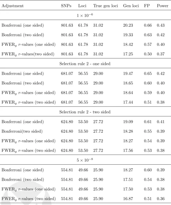
Adjustment Loci True gen loci Gen loci FP Power 1⇥10 6
Bonferroni (one sided) 61.78 22.75 22.49 0.80 0.48
Bonferroni (two sided) 61.78 22.75 21.34 0.74 0.46
FWERg r-values (one sided) 61.78 22.75 20.40 0.70 0.44 FWERg r-values (two sided) 61.78 22.75 19.09 0.62 0.41
Selection rule 2 - one sided
Bonferroni (one sided) 56.55 21.91 21.62 0.77 0.46
Bonferroni (two sided) 56.55 21.91 20.55 0.72 0.44
FWERg r-values (one sided) 56.55 21.91 20.54 0.71 0.44 FWERg r-values (two sided) 56.55 21.91 19.16 0.62 0.41
Selection rule 2 - two sided
Bonferroni (one sided) 53.50 21.35 21.02 0.71 0.45
Bonferroni (two sided) 53.50 21.35 20.09 0.67 0.43
FWERg r-values (one sided) 53.50 21.35 20.08 0.66 0.43 FWERg r-values (two sided) 53.50 21.35 19.21 0.62 0.41
5⇥10 8
Bonferroni (one sided) 49.66 20.19 19.95 0.68 0.43
Bonferroni (two sided) 49.66 20.19 19.16 0.65 0.41
FWERg r-values (one sided) 49.66 20.19 19.15 0.64 0.41 FWERg r-values (two sided) 49.66 20.19 18.37 0.61 0.39