Inhibition in Multiclass Classification
Ram ´on HuertaShankar Vembu
BioCircuits Institute, University of California, San Diego, La Jolla, CA 92093-0402, U.S.A.
Jos´e M. Amig ´o
Department of Statistics, Mathematics, and Computer Science, Universidad Miguel Hern´andez, Elche 03202, Spain
Thomas Nowotny
School of Informatics, University of Sussex, Falmer, Brighton BN1 9QJ, U.K.
Charles Elkan
Department of Computer Science and Engineering, University of California, San Diego, La Jolla, CA 92093-0404, U.S.A.
The role of inhibition is investigated in a multiclass support vector ma-chine formalism inspired by the brain structure of insects. The so-called mushroom bodies have a set of output neurons, or classification func-tions, that compete with each other to encode a particular input. Strongly active output neurons depress or inhibit the remaining outputs without knowing which is correct or incorrect. Accordingly, we propose to use a classification function that embodies unselective inhibition and train it in the large margin classifier framework. Inhibition leads to more robust classifiers in the sense that they perform better on larger areas of appro-priate hyperparameters when assessed with leave-one-out strategies. We also show that the classifier with inhibition is a tight bound to proba-bilistic exponential models and is Bayes consistent for 3-class problems. These properties make this approach useful for data sets with a limited number of labeled examples. For larger data sets, there is no significant comparative advantage to other multiclass SVM approaches.
1 Introduction
The question of what algorithms neural media use to solve challenging pat-tern recognition problems remains one of the most fascinating and elusive problems in the neurosciences, as well as in artificial intelligence. Percep-trons and artificial neural networks were originally inspired by neural com-putation, but thereafter, a new generation of powerful algorithms for pattern recognition returned to Fisher discriminant ideas and addressed the funda-mental question of minimizing the generalization error by using statistical principles. Kernel-based methods, in particular support vector machines (SVMs), became prevalent due to the convenience and simplicity of their algorithms. These methods became standard, and the original inspiration from neural computation faded away. The heuristics of neural integration, neural networks, plasticity in the form of Hebbian learning, and the regu-latory effect of inhibitory neurons were less needed, and the bioinspiration from neuroscience and AI fields grew increasingly distant from each other. We seek to bridge this gap and identify the similarities and, in some cases, equivalence between neural information processing and large mar-gin classifiers. We use the large marmar-gin classifier formalism and attempt to identify a correspondence to neural mechanisms for pattern recogni-tion, putting emphasis on the role of inhibition (Huerta, Nowotny, Garcia-Sanchez, Abarbanel, & Rabinovich, 2004; Huerta & Nowotny, 2009; O’Reilly, 2001). We use insect olfaction as our biological model system for two main reasons: (1) the simplicity and consistency of the structural organization of the olfactory pathway in many species and its similarity to the structure of a SVM and (2) the large body of knowledge concerning the location of learning in insects during odor conditioning, which matches the location of plasticity in SVMs.
The mushroom bodies in the brains of insects contain many classifiers that compete with each other. The mechanism to organize this competition such that a single winner (class) emerges is inhibition (Cassenaer & Laurent, 2012; Huerta et al., 2004; Nowotny, Huerta, Abarbanel, & Rabinovich, 2005; Huerta et al., 2009; O’Reilly, 2001). Each individual classifier exerts down-ward pressure on the rest, with a strength that has to be regulated. The SVM formalism provides a framework in which to understand the consequences of inhibition in multiclass classification problems.
The solution of the value of the inhibition using the SVM formalism leads to a unique solution, it is robust to parameter variations, and it is a tight bound of probabilistic exponential models. We also show simple se-quential algorithms to solve the problem using the sese-quential minimization algorithm (Platt, 1999a, 1999b; Keerthi, Shevade, Bhattacharyya, & Murthy, 2001) and a stochastic gradient descent (Chapelle, 2007; Kivinen, Smola, & Williamson, 2010). We provide efficient software for both algorithms written in C/C++ for others to experiment with (http://inls.ucsd.edu/ ∼huerta/ISVM.tar.gz).
We present extensive experimental results using a collection of easy and difficult data sets, some with heavily unbalanced classes. The data sets are from the UCI repository except for the MNIST digits data set. Results show that the inhibitory SVM framework generalizes better than the leading alternative methods with a small number of training examples. The mech-anism of inhibition provides robustness. The inhibitory models, for a large sample of meta parameters, outperform 1-versus-all SVMs and Weston-Watkins multiclass SVMs (Weston & Weston-Watkins, 1999). For large data sets when there is sufficient data to estimate the metaparameters by leave-one-out strategies, the ISVM does not provide a significant advantage. Moreover, in terms of Bayes consistency (Tewari & Bartlett, 2007), the inhibitory SVM is better than other methods with the exception of Lee, Lin, and Wahba (2004).
This letter starts by explaining the notation and the insect-inspired formalism of the inhibitory classifier, followed by a comparison to pre-vious methods using the same notation. Then we solve the formulation to write efficient and simple algorithms. We conclude with experimental results.
2 Insect Brain Anatomy
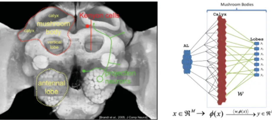
The three areas of the insect brain involved in olfaction are the olfactory receptor cells or sensors, the antennal lobe (AL) or feature extraction device, and the mushroom body (MB) or classifier (see Figure 1). When a gas is present, olfactory receptor cells feed this information into the AL, which extracts the features that will be classified by the MB.
The input, and hence the evoked feature patternx in the AL, can be associated with either a reward+1 or with punishment−1 at the level of the output of the MB that we denote byy. GivenN inputs, the problem consists of training the MB to correctly matchyi= f(xi)fori=1, . . . ,N.
The MB function consists of two phases (Heisemberg, 2003; Laurent, 2002): (1) a projection into an explicit high-dimensional space(x)named calyx and consisting of hundreds of thousands of Kenyon cell neurons (KC) and (2) a perceptron-like layer in the MB lobes (Huerta & Nowotny, 2009) where the classification function of each output neuron is implemented,
fk(x)= wk,(x) =jwk jj(x).1The inner product reflects the synaptic integration of KC outputs in MB lobe neurons. Huerta and Nowotny (2009) and Huerta et al. (2004) showed that simple Hebbian rules can solve dis-crimination and classification problems because they closely resemble the
1Note the distinction to the standard kernel trick with an implicit mapping of inputs.
Explicit mapping of inputs into a high-dimensional feature space was recently considered in Chang, Hsieh, Chang, Ringgaard, and Lin (2010) to speed up the training of nonlinear SVMs.
Figure 1: Illustration of the correspondence between the insect brain and ker-nel classification. (Left) Anatomical picture of the honeybee brain (courtesy of Robert Brandt, Paul Szyszka, and Giovanni Galizia). The antennal lobe is cir-cled in dashed yellow, and the MB is circir-cled in red. The projection neurons (in green) send direct synapses to the Kenyon cells in the calyx. The Kenyon cells carry the connectionswthat are the equivalent to the SVM hyperplane. (Right) Equivalent circuit representation in SVM language.
learning obtained by calculating the subgradient in an SVM framework. In particular, it can be shown that the change in the synaptic connections,w, is proportional toj(x). These rules are also equivalent to the perceptron algorithm, as Freund and Schapire (1999) showed.
In addition, the MB lobes contain hundreds of neurons that operate in parallel and compete via synaptic inhibition that they receive from each other, in addition to the input(x)from the calyx. The output neurons can, in principle, code for different stimulus classes. They can be situated in dif-ferent MB lobes specializing in difdif-ferent functions, and they are modulated by neuromodulators like dopamine, octopamine, and others that are the focus of intense research in neuroscience.
The concept of inhibition does not directly appear in the SVM literature, although a fairly large body of research on multiclass SVMs uses similar concepts. Our goal here is to directly integrate the concept of inhibition into the SVM formalism in order to provide a simple algorithm for multiclass classification.
3 The Inhibitory Classifier
Consider a training set of data points xi for i=1, . . . ,N whereN is the number of data points. Each point i belongs to a known classyˆi whose value is an integer in the range [1,L]. We first make a change of variables
from the vectoryˆto theN×Lmatrixy(called a coding matrix by Diettrich & Bakiri, 1995) defined by
yi j=
1 ifyˆi= j −1 otherwise,
(3.1)
that is,yijis 1 if the data pointxibelongs to the classj; otherwise the entry is−1.2
Next, we create a vectorχiasLconcatenations ofx
i, that is, χi=(x i,xi, . . . ,xi) Ltimes . (3.2)
If xi∈ M, then the number of components of χi is L·M. More gen-erally, given an arbitrary data point x∈ M, define E(M)⊂ LM to be the subspace of intrinsic dimension M built by vectors of the formχ= (x,x, . . . ,x)(xrepeatedLtimes). We say sometimes thatχ=(χ1, . . . , χLM) is the embedding of x into E(M). The inverse relation is given by
x=(χkL+1, χkL+2, . . . , χ(k+1)L)for anyk=0,1, . . . ,M−1.
When discussing SVMs, it is common to assume a nonlinear transforma-tion:M→Ffrom the original data spaceMto a feature vector space
Fin order to facilitate the separability of data points. Moreover, we assume thatF is endowed with a dot product ·,·:F×F→ . The inhibitory SVM proposed here uses a feature space that is the Cartesian product
FL=F× · · · ×F (L times). Correspondingly, we extend to a nonlin-ear transformation:E(M)→E(F), whereE(F)⊂FLis the subspace of dimension dimFbuilt analogously as before, by repeated concatenation of the first dimFcomponents, and
(χ)=((x), (x), . . . , (x)), (3.3)
whereχis the embedding ofxintoE(M). Furthermore, let
j:E(M)→
FLbe the composition ofwith the projection operator onto thejth coor-dinate subspace ofFLcorresponding to the classj, that is,
j(χ)=(0, . . . ,0, (x),0, . . . ,0). (3.4)
2There is a proposed generalization of the coding matrix (Allwein, Schapire, & Singer,
2000). For simplicity, we prefer to solve the problem of inhibitory classifiers in the frame-work of Diettrich and Bakiri (1995). The extension proposed by Allwein et al. (2000) is a possible generalization for the future.
To ease the notation, the indicesi,iwill refer henceforth to data points in M, while the indices j,j will refer to the classification classes. Their
ranges are thusi,i∈ {1, . . . ,N}and j,j∈ {1, . . . ,L}.
The new inhibitory classifier for a data pointxiand classj,fj:E(M)→ , has the form
fj(χi)= w, j(χi) −μw, (χi) = w, j(χi)−μ(χi), (3.5) wherew∈FL,w=0, is a hyperplane. Here·,·is the dot product inFL, defined as the sum of the dot products of corresponding projections onto each factor spaceF. The scalarμis the inhibitory factor and is the key nov-elty compared to other multiclass SVM methods because it is directly used in the evaluation of the classification function. As we will show, the value of the inhibitory factorμcan be derived directly from the minimization of the Lagrangian form and is data set independent. Note that
j fj(χi)= j w, j(χi) −μLw, (χi) (3.6) = w, (χi) −μLw, (χi) =(1−μL)w, (χi) for alli=1, . . . ,N.
The transformationsandjinherit many properties from the trans-formation function of standard SVMs, :M→F. In particular (see equations 3.3 and 3.4), (χi), (χi) =L· (x i), (xi), (3.7) j(χi), (χi ) = (xi), (xi), (3.8) j(χi), j(χi ) =I(j= j)(xi), (xi), (3.9) where the dot product·,·on the left-hand side of equations 3.7 to 3.9 is taken in the product space FL, while the dot product on the right-hand side is taken inF, and the indicator functionI(j= j)is 1 if j= j and 0 otherwise. The dot product(xi), (xi)can be computed effectively by a standard SVM kernel evaluationKii =K(xi,xi)= (xi), (xi). Thus, we can develop the inhibitory multiclass SVM formulation using the standard kernel trick.
The basic idea behind equation 3.5 is to trainfjclassifiers that inhibit each other by a factorμ, which is data set independent. In the current form, we seek a single winner by virtue of the matrixyij. However, the approach can
be used with data points assigned to multiple classes. All the subclassifiers
fjmust adjust, using the inhibitory factor, to classify the whole training set as well as possible. The conditions to have all the training points properly classified are
yi jfj(χi)≥1−η
i j,
whereηi j≥0 areN·Lslack variables.
Inhibition is not a new concept in machine learning. In particular, it has already been proposed in the context of energy-based learning via the so-called generalized margin loss (GML) function (LeCun, Chopra, Hadshell, Ranzato, & Jie, 2006). The wordinhibitionis not used explicitly in LeCun et al., but there are manifest similarities. The GML function represents the distance between the correct answer and the most offending incorrect answer. GML learning algorithms must change parameter values in order to make this distance be above a marginm. One can express the GML using our notation as
fGMLj (χi)= w, j(χi) −max
∀j=j w, j(χ
i). The goal of training is to achieveyi jfGML
j (χi)≥m−ηi j for allyi j=1, wheremis an arbitrary margin value. The inhibitory formulation that we propose replaces the max operation by a summation and a multiplicative factorμ. Thus, we retain differentiability, which is advantageous for sub-sequent developments. A second difference is that the SVM formulation requires margin constraints to be satisfied foryi j= −1. As we will see in the next few sections, these modifications allow us to create an effective, straightforward version of inhibition for SVMs.
Regular SVMs have been related to probabilistic exponential models (Canu & Smola, 2005; Pletscher, Soon Ong, & Buhmann, 2010). The in-hibitory SVM can remarkably also be connected to log-linear models. Using our notation in a log-linear model, the probability of the labeljgiven the data pointχand parameterswis
p(j|χ;w)= e
w,j(χ)
kew,k(χ) ,
where the indicesjandkrun over the classes 1 toL. Taking the logarithm of the previous expression gives
logp(j|χ;w)= w, j(χ) −log k
Lemma 1. Given f = (f1, . . . ,fL)∈ L, then a: log L k=1 expfk− 1 L L k=1 fk−logL≥0 (3.10) b: log L k=1 expfk− 1 L L k=1 fk−logL=0 for f1=· · ·= fLonly.
The proof can be found in appendix A. By applying lemma 1, one can write
logp(j|χ;w)≤ w, j(χ) −1
Lw, (χ) −logL, (3.11)
which is an equality if and only if fj:= w, j(χ) = w, k(χ) =: fk, for all 1≤ j,k≤L.
Note that most of the values ofw, j(χ)will be in the range [−1,1] due to the large margin optimization ofyi jfj(χi)≥1−η
i j. That means that the equality is a close bound top(j|χ;w)for most of theχi. This approximation to logp(j|χ;w) is similar to equation 3.5, whereμis in this case 1/L, as shown below in the derivation. The universality of the inhibitory factor is prevalent. The idea of inhibition can thus be expressed by a normalization factor that depends on the outcome of all classifiers.
4 The Primal Problem
The primal objective function is the sum of the loss on each training exam-ple and a regularization term that reduces the comexam-plexity of the solution (Vapnik, 1995; Muller, Mika, Ratsch, Tsuda, & Sch ¨olkopf, 2001). The relative weight of the regularization term is controlled by a constantC>0. The primal optimization problem can be expressed as
minimize E(w, μ)=12w2+Ci jηi j(w, μ)
subject to (i)ηi j(w, μ)≥0 (ii)yi jfj(χi)−1+η
i j(w, μ)≥0.
(4.1)
Thus, we have L·dimF+1 variables (w∈FL\{0} and μ∈ ) and 2NL constraints. This problem is not convex in general due to the dependence of ηi jonwandμ. Observe that fj(χi)also depends onwandμ(see equation 3.5). Ifdomη= ∩i jdomηi jdenotes the common domain of the mapsηi j, then the domain of the problem, equation 4.1, isD=(FL\{0} × )∩dom η. Moreover, we assume that all ηi j are continuously differentiable. For
practical purposes, the latter condition can be relaxed to hold except on a zero-measure set.
Consider the Lagrangian associated with equation 4.1:
L(w, μ,α,β)=1 2w 2 +C i j ηi j− i j βi jηi j (4.2) − i j αi j(yi j[w, j(χi) −μw, (χi)]−1+ηi j), (4.3) whereα=(αi j)∈ NL,β=(β
i j)∈ NL are the Lagrange multipliers. The Lagrange dual function (Boyd & Vandenberghe, 2004),
G(α,β)= inf
(w,μ)∈DL(w, μ,α,β), (4.4) then yields a lower bound on the optimal valuep∗of the primal problem, equation 4.1, for allαi j≥0 andβi j≥0.
Thus,G(α,β)is determined by the critical points ofL(w, μ,α,β)for each value ofαandβ. SinceLis aC1 function of all its variables, we take the partial derivatives ofLwith respect towandμand equate to zero in order to get its critical points:
w− i j (βi j−C+αi j)∂wηi j− i j αi jyi j j(χi)−μ(χi) =0 (4.5) − i j (βi j−C+αi j)∂μηi j+ i j αi jyi j w, (χi)=0. (4.6)
According to the implicit function theorem, the solutions of equations 4.5 and 4.6 provide local functionsw=wcrit(α,β)andμ=μcrit(α,β), except possibly for a zero measure set (actually a manifold) comprising those αi j, βi jvalues that make the Jacobian determinant vanish:
detJ(w, μ,α,β)=0. (4.7)
Moreover, these functions are continuously differentiable on account of all functional dependencies in equations 4.5 and 4.6 being continuously differ-entiable. Note that the infimum in equation 4.4 is taken over points(w, μ)∈
D, but(wcrit(α,β), μcrit(α,β))need not be inDfor all values ofαandβthat parameterize the implicit solutions. This being the case, we have that
G(α,β)=L(wcrit(α,β), μcrit(α,β),α,β) (4.8) for allα,βsuch that detJ(w, μ,α,β)=0 and(wcrit(α,β), μcrit(α,β))∈D.
For our purposes, it will suffice to study the critical points on the
NL-dimensional plane α+β−C=0(intersection of theNLhyperplanes αi j+βi j=C), whereC=(Ci j)∈ NLwithCi j=C>0 for alli,j.
Lemma 2. From equations 4.5 and 4.6, it follows that
μcrit(α,C−α) = 1 L (4.9) and wcrit(α,C−α) = i j αi jyi j Ψj(χi)− 1 LΨ(χ i) (4.10)
for allα= (αi j)∈ NLsuch that
i jαi jyi jΨ(χi)= 0.
The proof can be found in appendix B. Note thatC in equation 4.9 is fixed but arbitrary. If follows thatμcrit(α,β)does not depend on eitherαor β; hence,
μcrit(α,β)= 1
L. (4.11)
Theorem 1. Let E(w∗, μ∗)be the optimal value of the primal problem, equation 4.1. Then
μ∗= 1
L.
The proof can be found in appendix C. The optimal solution μ= 1 L renders the average output of all subclassifiers to be 1Lw, (χi) =
1 L
jw, j(χi). The inhibitory factor turns out to be data set independent. Furthermore, from equation 3.6, it follows thatj fj(χi)=0.
The next step consists of putting all the constraints back into the classifier given by equation 3.5 to obtain
fj(χ)= N i=1 L j=1 αijyijK(xi,x)(I(j= j)−1/L)≡ fj(x), (4.12)
whereχ=(x,x, . . . ,x)∈E(M). To decide which class to choose for a given data pointx, one uses the same decision function as in Weston and Watkins (1999) and Crammer and Singer (2001):
arg max
It is important to note that during classification, all of the fj(x) can be simplified because they are shifted by the same amount, that is,
fj(χ)= N i=1 L j=1 αijyijK(xi,x)I(j= j) −1 L N i=1 L j=1 αijyijK(xi,x)= ˜fj(x)+G(x). (4.14)
We can simplify the evaluation on the test set by just calculating ˜ fj(x)= N i=1 αijyijK(xi,x) (4.15)
and selecting the class as arg max
j fj(x)=arg maxj ˜
fj(x). (4.16)
5 Previous Integrated Multiclass Formulations
This section places the new inhibitory SVM in the context of previous work. As described in section 1, the most common approach to multiclass classi-fication is to combine models trained for a set of separate binary problems. A few previous approaches have integrated all classes into a single formu-lation. Generally, for classj, the output of the integrated approaches uses the classification function
fj(χ)= w, j(χ) +bj
wherebj is a bias term, with decision function 4.13. Weston and Watkins (1999) were the first to put multiclass SVM classification into a single for-mulation. Using our notation, they solved the problem
min w,η E= 1 2w 2+C i js.t.yi j=1 ηi j, (5.1)
but with different constraints,
w, j(χi)−j(χi)
for alljsuch thatyi j=1 and for all jsuch thatyi j= −1, wherebj,bj are bias terms andηi j≥0. The constraints imply that the SVM scores of all data points belonging to a given class need to be greater than the margin (see appendix E for details).
The large number of constraints hinders solving the quadratic program-ming problem. Crammer and Singer (2001) proposed to reduce the number of slack variables by solving
min w,η E= 1 2w 2+C i ηi (5.2) with constraints w, j(χi)−j(χi) +I(yi j=yi j)≥1−ηi
for alljsuch thatyi j=1,j= jand for all data pointsi. The main differences with respect to Weston and Watkins (1999) are the reduced number of slack variables (see appendix F for details).
Tsochantaridis, Joachims, Hofmann, and Altun (2005) propose solving a similar problem as in equation 5.2 by rescaling the slack as
w, j(χi)−j(χi)
≥1− ηi (yi j,yi j)
for all j such that yi j=1. The function (yi j,yi j) allows the loss to be penalized in a flexible manner, with(1,1)=0. A second version proposes rescaling the margin as
w, j(χi)−j(χi)
≥(yi j,yi j)−ηi.
Both approaches lead to similar accuracies on test sets, as shown in Tsochan-taridis et al. (2005).
A remarkable approach is the formalism proposed by Lee et al. (2004) where the authors rewrite the constraints to match the Bayes decision rule (see section 10 for details) such that the most probable class of a particu-lar exampleχ is the same as the one obtained by minimizing the primal problem. Lee and coauthors solve constraints as
−w, j(χi)≥ 1
such thatjis chosen from the set{j∈ {1,L},s.t.yi j=1}with the additional constraintw, (χi) =0. These constraints pose a cumbersome optimiza-tion problem but yield Bayes consistency (Tewari & Bartlett, 2007).
Table 1 presents a summary of the constraints used in each of the de-scribed methods. The main difference between our inhibitory multiclass method and the methods just described is in the way the classifier for class
j is compared to the other classifiers. The inhibitory method essentially compares to the average of the outputs of all classifiers, while the previous methods perform pairwise comparisons. The second important difference of the inhibitory method is that inhibition is incorporated directly into the classification function itself.
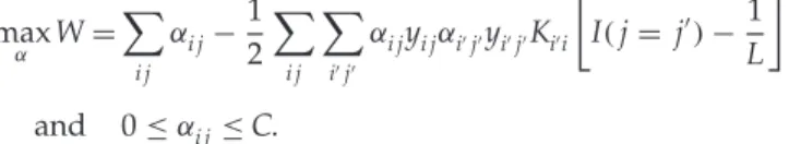
6 The Dual Problem of the Inhibitory Multiclass Problem
The dual problem is obtained by replacing all the constraints given by equations 4.9 and 4.10 with the solutionμ=1/Lin the Lagrangian, equa-tions 4.2 and 4.3, which yields the dual cost function,W. This cost func-tion has to be maximized with respect to the Lagrange multipliers,αi j, as follows: max α W= i j αi j−1 2 i j ij αi jyi jαijyijKii I(j= j)−1 L and 0≤αi j≤C.
The double index notation inαi jand elsewhere is inconvenient to compare with previous published work and with the primal formulation explained in the following sections. Thus, we change the notation fromi,jto a new indexkrunning from 1 toN·L. Thus, we order theαi j’s lexicographically: α1,1, . . . , α1,L, α2,1, . . . , α(N−1),L, αN,1, . . . , αN,L. With the new notation, we can write the dual problem as
max α W= k αk− 1 2 k k αkykαkykGkk (6.1) and 0≤αk≤C, (6.2) wherek,k=1, . . . ,N·Land Gkk=Kk−1 L +1, k−1 L +1 I[kmodL]=kmodL− 1 L . (6.3)
T able 1: Summary of the Constraints for S everal Integrated SVM M ulticlass Formulations. Method Constraints N umber o f C onstraints Bayes C onsistency W eston and W atkins, 1999 w , j ( χi ) − j ( χi ) + ( bj − bj ) ≥ 2 − ηij N · ( L − 1 ) L < 3 Crammer and Singer ,2001 w , j ( χi ) − j ( χi ) + I ( yij = yij ) ≥ 1 − ηi N · LL < 3 T sochantaridis et al., 2005, slack rescaling w , j ( χi ) − j ( χi ) ≥ 1 − ηi / ( yij , yij ) N · LL < 3 T sochantaridis et al., 2005, mar g in re scaling w , j ( χi ) − j ( χi ) ≥ ( yij , yij ) − ηi N · LL < 3 Lee et al., 2004 w , j ( χi ) ≥ 1 L − 1 − ηij and w , ( χi ) = 0 N · LL ≥ 2 Inhibitory multiclass (ISVM) yij w , j ( χi ) − μ ( χi ) ≥ 1 − ηij N · LL < 4
0, . . . ,N−1, and k=0, . . . ,N L−1, then the following kernel call is suggested: Gkk=Kk L, k L I[kmodL]=kmodL− 1 L . (6.4)
The Karush-Kuhn-Tucker (KKT) conditions for this problem can be cal-culated by constructing the Lagrangian from the dual as in Keerthi et al. (2001): L= − k αk+ 1 2 k k αkykαkykGkk− k ukαk− k lk(C−αk), 0≤αk≤C, uk,lk ≥0, which leads to yiEi−ui+li=0, ui,li≥0, αkuk=0, lk(C−αk)=0,
whereEi= fi−yiand fi=kαkykGki. We obtain the standard KKT condi-tions for the SVM training problem:
yiEi≥0 forαi=0, (6.5)
yiEi=0 for 0< αi<C, (6.6)
yiEi≤0 forαi=C. (6.7)
It is useful to define a new variableVi=yiEithat indicates the proximity to the margin and saves computation time.
7 Stochastic Sequential Minimal Optimization
Prior to the first sequential minimal optimization (SMO) methods (Platt, 1999a, 1999b), the quadratic programming algorithms available at the time made SVMs unfeasible for large-scale problems. The straightforward im-plementation of SMO enabled a significant thrust of developments and improvements (Keerthi et al., 2001). The multiclass problem investigated in equations 6.1 and 6.2 has an advantage due to the absence of the constraint
kαkyk=0, which is typical in the dual SVM formulation. This constraint appears after solving the primal problem for the biasbof the classifier. It is avoidable in the multiclass problem due to the mutual competition among the classifiers by means of the inhibitory factorμ.
The idea of optimizing the quadratic function for a pair of multipliers is needed because one cannot modify the values of a single multiplier without violating the constraintkαkyk=0 (Platt, 1999a, 1999b). In the inhibitory SVM, a single multiplier can be modified at a time. The analytical solution for a single multiplieriis derived from
W =constant+αi−1 2Giiα 2 i −αiyi fi−αioldyiGii,
whose solution is obtained from∂∂αW
i =0 to yield 1−Giiαi−yifi−αioldyiGii=0.
This can be rewritten as αi= αold i + 1 Gii 1−yiEi, (7.1) whereαold
i is the value of the multiplier in the previous iteration. Every time anαiis updated, each error updates according toEj(t+1)=Ej(t)+(αi− αold
i )yiGi j. In terms of the margin variableVi, one can write
Vj(t+1)=Vj(t)+(αi−αiold)yiyjGi j for j=1, . . . ,N L. (7.2)
The randomized SMO algorithm is given in algorithm 1. One can im-prove the performance of the algorithm by remembering the indices of the multipliers that violate the KKT conditions. Then, instead of choosing among all possible multipliers, one chooses among those that need to be changed. The KKT distance function in algorithm 1 is
KKTdistance(Vi, αi)= ⎧ ⎪ ⎪ ⎪ ⎪ ⎨ ⎪ ⎪ ⎪ ⎪ ⎩ −Vi if Vi<−T and αi< , Vi if Vi>T and αi>C−, |Vi| if |Vi|>T and < αi<C−, 0 rest of cases.
Above,Tis the resolution of the proximity to the KKT condition, which we typically fix to 10−3as originally proposed by Platt, andis the numerical
Algorithm 1: Stochastic SMO Algorithm. t:= 1
αi:= 0 andVi:=−1 fori= 1, . . . , NL
do{
Choose one index fromk∈[1, . . . , NL]. αnew=αk−GVkkk,
αnew= max{0, αnew}andαnew= min{C, αnew} Initialize the KKT distance:KKT:= 0 loop over alli= 1, . . . , NL
Vi:=Vi+ (αnew−αk)yiykGik KKT :=KKT+KKT distance(Vi, αi) end loop αk=αnew KKT:=KKT /(NL) t:=t+ 1 }while (KKT > θ)
Nis the number of data points,Lis the number of classes, andθ is the termi-nation threshold, which we generally set to the same value as the toleranceT (10−3).
Note:
resolution that depends on the machine precision that we typically set to 10−6. Generally, for all data sets tested, one can stop the algorithm early without impairing accuracy significantly.
8 Stochastic Gradient Descent in Hilbert Space
Synaptic changes do not occur in a deterministic manner (Harvey & Svo-boda, 2007; Abbott & Regehr, 2004). Axons are believed to make additional connections to dendrites of other neurons in a stochastic manner, suggest-ing that the formation or removal of synapses to strengthen or weaken a connection between two neurons is best described as a stochastic process (Seung, 2003; Abbott & Regehr, 2004). On the other hand, in recent times, variants of stochastic gradient descent (SGD) have been used to solve the SVM problem in the primal formulation (Bottou & Bousquet, 2008; Zhang, 2004; Shalev-Shwartz, Singer, & Srebro, 2007). The algorithms obtained for the modification of the synaptic weightswresemble closely Hebbian learn-ing or perceptron rules. We are primarily deallearn-ing with nonlinear kernels, so let us bridge the dual formulation with stochastic gradient descent using a Hilbert space.
Let us rewrite the primal formulation in equation 4.1 using a reproducing kernel Hilbert space (RKHS) as proposed in Chapelle (2007) and Kivinen et al. (2010). LetSbe the training data set. For our specific problem, the RKHS
H= {f:S→ }has a kernelG:S×S→ with a dot product·,·Hsuch thatG(·, χ ), fH= f(χ ), with χ∈Sand f ∈H. The primal formulation
then can be expressed as min f∈HE=minf∈H 1 2f 2 H+C NL i=1 max{0,1−yif(χi)} =min f∈H 1 2f,fH+C NL i=1 max{0,1−yif,G(χi,·)H} . (8.1)
The formal expression offis a linear combination of the kernel functions such that f(χ)=NLi=1αˆiG(χi,χ). In appendix D we show how the updating rule is derived as ˆ αi(t+1)=(1−η)αˆi(t)+ηCyi1(yift(χi)−1), (8.2) with 1(u)= ⎧ ⎪ ⎪ ⎨ ⎪ ⎪ ⎩ 1 ifu<0 0 ifu>0 [0,1] ifu=0 , (8.3)
andη is the learning rate. For the evaluation of ft(χ)we use the kernel derived from the Lagrange multipliers function given by equation 6.3 be-cause we know from the minimization of the Lagrangian thatμ=1/L. The correspondingiindex ofχis the one that verifiesχ=χiin the training set. For stochastic updating, it is convenient to track the evolution of the margin proximity variableVi=yift(χi)−1 every time a coefficientαˆ
iis changed:
Vj(t+1)=Vj(t)+yi(αˆi(t+1)− ˆαi(t))G(χi,χj) for j=1, . . . ,NL,
which is very similar to equation 7.2 obtained in the dual form.
Many approaches using stochastic gradient descent use a scaling factor in the learning rate proportional to (1/iteration number) in order to guarantee convergence (Zhang, 2004; Shalev-Shwartz et al., 2007). We propose here a different approach that leads to an algorithm that is almost equivalent to the stochastic SMO method. As in that method, we make use of the KKT conditions, which requires computing the current state of training at each iteration. Note that the variableViprovides guidance concerning distance to the margin.
If the algorithm chooses the indexk, then the changeαˆk(t+1)− ˆαk(t)= kis derived from
Note: t:= 1
αi:= 0 andVi:=−1 fori= 1, . . . , NL
do{
Choose one index fromk∈[1, . . . , NL]. αnew= ˆαk−ηeffyVkkG(tkk)
αnew= min{C, αnew}andαnew= max{−C, αnew} Initialize the KKT distance:KKT := 0
loop over alli= 1, . . . , NL Vi:=Vi+yi(αnew−αˆk)Gik KKT :=KKT+KKT distance(Vi, yiαˆi) end loop KKT :=KKT /(NL) ˆ αk=αnew t:=t+ 1 }while (KKT > θ)
Algorithm 2: Stochastic Gradient Descent (SGD) with Endogenous Learning Rate.
N is the number of data points,Lis the number of classes,ηeff is the learning
rate, and θ is the stopping criterion. Note that this algorithm needs to compute theVi
values.
so
k= −
Vk(t)
ykG(χk,χk), (8.4)
assuming thatG(χk,χk)=0. We combine equations 8.4 and 8.2 to obtain the learning rateηthat would take the data pointkexactly to the margin as
η(t)= Vk
ykG(χk,χk)λαˆ
k(t)−yk1(Vk) .
To avoid the computation inherent in the previous formula one can changekto
k= −ηe f f
Vk(t)
ykG(χk,χk). (8.5)
Whenηe f f =1, the update takes data pointxto the margin.
When we use ηe f f =1, we recover the SMO solution given in equation 7.1. The corresponding SGD algorithm is presented in algorithm 2. Algorithms 1 and 2 are almost identical. C++implementations of both al-gorithms can be found in the software package ISVM.
When making a prediction for a test example using fj(χ)=
NL
i=1αˆ∗iG(χi,χ), we replace G(χi,χ) by K(xi,x)(I(j= j)−1/L)≡ fj(x), which means that we need to makeLevaluations for each data point from
j=1, . . . ,Land select the one with the largest margin. This procedure is equivalent to equations 4.12 and 4.13.
The primal and the dual formalism lead to an almost identical algorithm for the inhibitory multiclass problem. A major appealing feature of the algorithms is the simplicity of their implementation.
9 Experimental Robustness
In this section we show experimentally that the inhibitory SVM (ISVM) method generally achieves better generalization than other multiclass SVM methods for small training set sizes. With large training sets, all methods converge to similar levels of accuracy, and it is not possible to obtain a clear distinction between methods. Rifkin and Klautau (2004) and Hsu and Lin (2002) showed that the performance of one-versus-all and one-versus-one approaches is good on many occasions with faster training times than the rest.
For this investigation, we use a gaussian kernel as exp−γx−x2/M. Then we have a pair of metaparametersC>0 andγ >0 to investigate. The key issue, in terms of robustness, is to determine whether the in-hibitory SVM leads to better average performance than 1-versus-all and Weston-Watkins multiclass approaches for any pair (C, γ ). It is obviously not possible to cover the whole space of metaparameters, but one can sam-ple it and get estimates. Our sampling methodology picks the best models at different percentile cuts—10%, 25%, and 50%—because one expects to explore parameter areas with a higher likelihood of achieving better per-formance. Thus, we ran an empirical leave-one-out verification strategy scanning the three hyperparameter valuesγ =5,10 and varyingC from 0.1 to 100 at steps of 0.5. The lower boundC=0.1 is set because for small data sets, the SVM evaluation functions hardly reach the margin, and the performance drops considerably for all the methods. Note also that since we discard all solutions below the 50% performance, we do not explore these solutions. We used the same stochastic SMO algorithms and the same C++ implementation for 1-versus-all, Weston-Watkins, and ISVM. Note that the only difference in the methods is the factors multiplying the kernel:K(xi,xi)(I(j= j)−1/L)for ISVM,K(xi,xi)I(j= j)for SVM, and
K(xi,xi)(Lk=1(I(j= j)+yik2+1yik2+1))for Weston-Watkins.
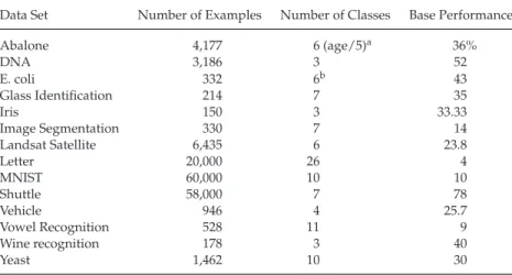
In order to demonstrate the higher robustness of inhibition in a system-atic manner we ran comparisons in 14 datasets for several different sizes of the training setNs=50, 100, 150, 200, 500 (see Table 2). Then we took an average of 100 random samples of each data set of sizeNs. In Table 3, we report the results of pooling the leave-one-out performances for a grid of
Table 2: Summary of the Data Sets Used for Robustness Calculation.
Data Set Number of Examples Number of Classes Base Performance
Abalone 4,177 6 (age/5)a 36% DNA 3,186 3 52 E. coli 332 6b 43 Glass Identification 214 7 35 Iris 150 3 33.33 Image Segmentation 330 7 14 Landsat Satellite 6,435 6 23.8 Letter 20,000 26 4 MNIST 60,000 10 10 Shuttle 58,000 7 78 Vehicle 946 4 25.7 Vowel Recognition 528 11 9 Wine recognition 178 3 40 Yeast 1,462 10 30
Notes: We indicate the number of examples, the number of classes, and the worst possible performance by choosing as the default answer the most probable class in the data sets.
aThis data set predicts age from 1 to 29. It is more of a regression problem. Thus, we
predict age bands dividing age by 5.
bimL and imS classes removed because they have two examples each.
metaparameters using the gaussian kernel, exp(−γx−x2/M)). The 10% best models were pooled and the average calculated. The same procedure is carried out for the 25% and 50% best to illustrate the drop of performance as we increased the area of the parameter set.
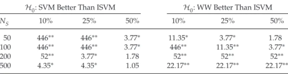
The main conclusion from this assessment is that the average mance for areas of parameter values that provide a near-optimal perfor-mance is higher for the ISVM than for the 1-versus-all and Weston-Watkins. In general, one can see that for small data sets, the performance of the ISVM is better, although it curves down for a higher number of examples. The Weston-Watkins method is competitive for small data sets but then loses performance for a higher number of samples. In general, the ISVM demon-strates better overall robustness and performance for small data sets. To summarize the results and add interpretation to the table, we tested the null hypothesesH0that either the SVM or WW method has average perfor-mance better than or equal to the ISVM method. We performed a maximum likelihood ratio test (Dempster, 1997; Rodriguez & Huerta, 2009) as it has, according to the Neyman-Pearson lemma, optimal power for a given sig-nificance niveau (Neyman & Pearson, 1933). For the 14-trial (data set) test,
H0can be rejected at significance niveau 5% if the likelihood ratioLis larger thanc=3.77. Table 4 summarizes the results by showing that most of the time we can reject theH0hypothesis. If, on the other hand, one runs the test against the alternative hypothesisH1“ISVM is better than or equal to SVM or WW,” it cannot be rejected in any of the cases.
T able 3: A verage P erformance Comparison for ISVM, 1-V ersus-All and W eston-W atkins U sing 14 Data S ets and Running LOO on 100 Random Samples for E ach Data Set. Inhibitory SVM 1-V ersus-All W eston-W atkins Data Set NS 10% 25% 50% 10% 25% 50% 10% 25% 50% Abalone 50 61.43 % 60.69 % 60.09 % 60.83% 59.69% 58.85% 60.07% 59.47% 59.10% Abalone 100 66.55 65.91 65.16 65.47 64.13 63.12 64.18 64.12 64.06 Abalone 200 67.00 66.61 66.08 65.97 65.07 64.08 63.63 63.61 63.58 Abalone 500 67.77 67.48 67.09 67.63 66.87 65.79 64.24 64.23 64.22 DNA 50 49.59 49.25 49.14 49.28 49.13 49.08 49.77 49.18 47.99 DNA 100 54.08 54.04 54.02 54.04 54.04 54.01 52.78 52.29 52.02 DNA 200 56.24 56.19 56.16 56.20 56.18 56.13 53.33 53.18 52.66 DNA 500 60.90 60.87 60.82 60.92 60.90 60.84 53.57 53.57 53.56 E. coli 50 82.05 81.24 80.25 80.60 79.04 78.44 81.02 80.83 80.58 E. coli 100 84.06 83.60 82.78 83.23 81.56 80.55 82.97 82.90 82.78 E. coli 200 87.02 86.52 85.78 86.32 84.85 83.41 85.34 85.32 85.30 Glass 50 64.52 64.36 64.13 63.82 63.29 62.83 61.00 60.97 60.92 Glass 100 71.92 71.80 71.35 71.08 70.79 70.41 63.99 63.97 63.94 Glass 200 75.23 74.78 74.37 75.27 74.79 74.12 65.79 65.79 65.76 Iris 50 89.45 89.37 89.26 89.31 89.14 88.91 87.19 86.54 85.81 Iris 100 91.94 91.86 91.65 91.88 91.55 91.38 90.88 90.20 89.13 Iris 140 93.16 93.03 92.81 92.95 92.71 92.54 92.39 92.27 91.95
T able 3: Continued. Inhibitory SVM 1-V ersus-All W eston-W atkins Data Set NS 10% 25% 50% 10% 25% 50% 10% 25% 50% L. Sat 50 82.43 82.24 81.99 81.91 81.56 81.44 82.37 82.30 82.24 L. Sat 100 83.00 82.88 82.64 82.61 82.33 82.24 83.00 82.97 82.93 L. Sat 200 85.49 85.38 85.16 85.17 84.86 84.75 84.81 84.80 84.79 L. Sat 500 89.08 88.74 88.47 88.58 88.34 88.26 85.94 85.93 85.93 Letter 50 30.68 30.65 30.61 30.64 30.64 30.63 30.00 30.00 30.00 Letter 100 40.69 40.57 40.27 39.95 39.93 39.91 39.98 39.98 39.98 Letter 200 51.53 51.46 51.35 50.96 50.95 50.94 52.41 52.41 52.40 Letter 500 66.54 66.45 66.27 64.57 64.44 64.39 68.09 68.08 68.08 MNIST 50 53.76 53.76 53.38 53.80 53.80 53.72 51.88 51.86 51.85 MNIST 100 67.22 67.22 66.50 67.18 67.18 67.03 64.58 64.58 64.58 MNIST 200 77.53 77.53 76.76 77.51 77.51 77.34 75.40 75.40 75.40 MNIST 500 85.82 85.80 85.08 85.62 85.61 85.44 83.65 83.65 83.65 Segment 50 77.72 77.63 77.53 77.71 77.58 77.46 75.35 75.02 74.65 Segment 100 83.74 83.71 83.61 83.90 83.82 83.67 81.86 81.82 81.77 Segment 200 87.86 87.79 87.63 87.85 87.82 87.74 85.48 85.46 85.44 Shuttle 50 90.85 90.84 90.83 90.76 90.76 90.72 90.22 90.15 90.08 Shuttle 100 94.31 94.29 94.18 93.95 93.94 93.92 93.91 93.89 93.84 Shuttle 200 97.02 97.01 96.95 96.88 96.85 96.81 96.29 96.28 96.28 Shuttle 500 98.60 98.53 98.41 98.40 98.30 98.25 97.68 97.68 97.67
T able 3: Continued. Inhibitory SVM 1-V ersus-All W eston-W atkins Data Set NS 10% 25% 50% 10% 25% 50% 10% 25% 50% Ve h ic le 50 61.06 61.02 60.70 60.91 60.89 60.69 58.13 57.86 57.56 V ehicle 100 66.28 66.28 65.99 66.14 66.14 66.03 63.36 63.14 62.86 V ehicle 200 70.13 70.07 69.85 70.01 69.97 69.88 67.63 67.58 67.51 V ehicle 500 75.26 74.36 73.89 74.66 74.13 73.95 71.23 71.16 71.03 V o wel 50 46.61 46.61 46.48 46.60 46.60 46.57 46.76 46.76 46.76 V o wel 100 61.61 61.58 61.37 61.48 61.48 61.45 62.08 62.07 62.06 V o wel 200 77.73 77.65 77.54 77.78 77.77 77.74 77.76 77.75 77.75 V o wel 500 95.00 94.87 94.83 95.20 95.20 95.16 94.52 94.52 94.52 W ine 50 93.17 93.17 93.12 93.16 93.16 93.12 93.32 93.30 93.25 W ine 100 94.26 94.23 94.21 94.21 94.20 94.20 94.24 94.22 94.20 W ine 150 95.29 95.29 95.27 95.29 95.29 95.28 94.85 94.82 94.81 Ye as t 50 48.36 47.60 46.98 47.21 46.39 46.09 47.99 47.71 47.44 Y east 100 52.57 51.63 50.74 50.66 49.11 48.56 51.58 51.57 51.55 Y east 200 55.00 54.28 53.16 53.01 50.55 49.60 53.06 53.05 53.02 Y east 500 60.26 59.27 57.75 55.92 51.95 49.88 54.89 54.89 54.89 Notes: The k ernel u sed is exp ( − γ x − x 2/ M )) , such that the radial basis functions ar e n ormalized to the n umber o f featur es. The performance shown is b ased on the leave-of-out calculation o f Ns samples run over 100 dif fer ent realizations. T he performances of all explor ed metaparameters for C = 0 . 1t o5 0a n d γ = 5 , 10 ar e p ooled and sorted. The table shows the average performance of the 10%, 25%, and 50% best models. In most of the cases, the inhibitory SVM o utperforms the re st, w ith W eston-W atkins being competitive for smaller sizes and 1-versus-all b ecoming competitive for Ns ≥ 200.
Table 4: Likelihood Ratio Values Using the 14 Data Sets.
H0: SVM Better Than ISVM H0: WW Better Than ISVM
NS 10% 25% 50% 10% 25% 50%
50 446∗∗ 446∗∗ 3.77∗ 11.35∗ 3.77∗ 1.78 100 446∗∗ 446∗∗ 3.77∗ 446∗∗ 11.35∗∗ 3.77∗
200 52∗∗ 3.77∗ 1.78 52∗∗ 52∗∗ 52∗∗
500 4.35∗ 4.35∗ 1.05 22.17∗∗ 22.17∗∗ 22.17∗∗ Notes: c-values≥3.77 reflect a significance niveau ofPr(L≥c|H0)≤0.05 (*) and c values
≥11.35 reflect a significance ofPr(L≥c|H0)≤0.01 (**). For the 9 data sets with size 500,
the rejection thresholds are 4.35 and 22.17. Thus, the null hypothesis can be rejected in most cases. If the null hypothesis is reversed (ISVM better than SVM and ISVM better than WW), then we cannot reject it in any of the cases.
In terms of training time, the Weston-Watkins algorithm is the fastest of all the methods and runs eight times faster than the ISVM on the leave-one-out error task fromC=0.1 to 50 for all the data sets and two times faster than the 1-versus-all. The three methods were implemented using the same code and the same stochastic SMO, so the better performance and robustness come with a cost in training, although there is not significant time difference in execution.
10 Bayes Consistency
Our overall goal is to find a classification functionfwith a minimal probabil-ity of misclassificationR(f)(Lugosi & Vayatis, 2004). In a multiclass setting (Tewari & Bartlett, 2007), given the posterior probabilitiespj≡p(o=yj|x)
withjlabeling allLoutput classes and given the outputsf∗j(x)after training, arg maxj f∗j must match arg maxjpj. In other words, the classifier function,
f= {f1, . . . ,fL} must select the most probable class (or the most proba-ble classes if several classes have equal probability). This condition is called classification calibration, and theorem 2 in Tewari and Bartlett (2007) asserts that classification calibration is necessary and sufficient for convergence to the optimal Bayes risk. Tewari and Bartlett use
inf
f R(f)=inff
j
pjh(fj), (10.1)
whereh(fj)is the cost function without the regularization term. The in-hibitory SVM has
h(fj)=[1−(fj− ˆf)]++
i=j
Algorithm 3: Monte Carlo Algorithm to Check Bayes Consistency. c:= 1,N:= 1,L:=L∗
do{
Choosep∈( +)Land normalizepi:=pi/ jpj
Find the infimum of ipih(fi)
if arg minih(fi) = arg maxipithenc:=c+ 1 N:=N+ 1
}while (N≤Nmax )
risk=1−N c
max
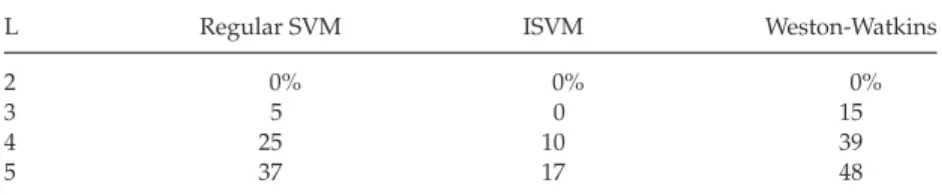
Table 5: Monte Carlo Simulation of Consistency Using 100,000 Runs.
L Regular SVM ISVM Weston-Watkins
2 0% 0% 0%
3 5 0 15
4 25 10 39
5 37 17 48
Notes: We found 0% consistency errors, not surprisingly, for binary problems. The ISVM is also consistent forL=3, and then it becomes inconsistent. Note that the probability of having a harder problem increases with the number of classes.
where fˆ= 1 L
i fi and fj∈ . The problem, equation 10.1 is thus equiv-alent to solving a linear problem with infzjpjzj,wherez takes all the admissible values induced byf∈ L. The consistency condition is
arg min
i zi=arg maxi pi.
Tewari and Bartlett (2007) analyze the consistency of several multiclass classifiers, which requires characterizing the induced sets ofzbyf. Because the proofs can be cumbersome due to the topological complexity of the intersecting hyperplanes induced byf, Monte Carlo simulations are a viable alternative to quickly evaluate the consistency of a classifier. Algorithm 3 is a straightforward algorithm.
Table 5 lists the consistency risks observed. An advantage of the ISVM is its consistency for 3-class problems and a lower probability of reaching inconsistencies forL>3.
11 Conclusion
In this letter, we have developed a new variation on the support vec-tor machine theme using the concept of inhibition that is widespread in
animal neural systems (Cassenaer, & Laurent, 2012). The main engineering advantage of inhibition is the ability to achieve better average accuracy for a broad metaparameter space with a small number of training examples, shown across multiple learning tasks. This success of the inhibitory SVM method is reminiscent of the low number of examples that insects need to learn odor recognition (Smith, Abramson, & Tobin, 1991; Smith, Wright, & Daly, 2005).
The underlying reason that ISVMs perform better in the cases reported here appears to be that the inhibition provides a wider area of the hyper-parametersC andγ that are close to the optimum, making finding good hyperparameters easier. Consistency analysis shows that ISVM are still con-sistent for 3-class problems and show a smaller percentage of inconsisten-cies overall. The ISVM can be made consistent by eliminating the positive examplesyi j=1 from the primal function, but this point is left for further analysis. Finally, it is important to emphasize that by using lemma 1, we show that log-linear models are almost equivalent to the inhibitory SVM framework, reflecting the universality of inhibition in different classification formalisms.
Appendix A: Proof of Lemma 1
(a) Jensen’s inequality for convex functions applied to the exponential map reads (see section 3.1.8 of Boyd & Vandenberghe, 2004)
1 L L k=1 expfk ≥exp 1 L L k=1 fk (A.1)
for all f1, . . . ,fL∈ . Use the increasing monotonicity of the logarithm function to derive log1 L+log L k=1 expfk ≥ 1 L L k=1 fk, which is equation 3.10.
(b) From the graphical interpretation of Jensen’s inequality, it is plain that the equality in equation A.1 holds if and only if f1= · · · = fL, that is, if all the components offare equal.
Appendix B: Proof of Lemma 2
Sinceαi jandβi jare arbitrary in equations 4.5 and 4.6, setβi j=C−αi j to get the simplified expressions
w− i j αi jyi jj(χi)−μ(χi)=0, (B.1) i j αi jyi j w, (χi)=0. (B.2)
Next solve forwin equation B.1 and replace in equation B.2 to obtain 0= i j ij αi jyi jαijyijj(χi )−μ(χi), (χi) = i j ij αi jyi jαijyij j(χi ), (χi) −μ(χi), (χi) = i j ij αi jyi jαijyij (xi), (xi) −μL(xi), (xi) =(1−μL) ij αijyij(xi), i j αi jyi j(xi) =(1−μL) i j αi jyi j(xi) 2 , (B.3)
where we employed equations 3.7 to 3.9. Henceμ= 1 Lif
i jαi jyi j(xi)=
0. Finally, note that the latter inequality holds true if and only if
i jαi jyi j(χi)=0in virtue of equation 3.3.
Appendix C: Proof of Theorem 1
LetE(w∗, μ∗)be the optimal value of the primal problem, equation 4.1. (i) In the generic case, detJ(w∗, μ∗,α∗,β∗)=0. Thenw∗=wcrit(α∗,β∗)
and
μ∗=μ
crit(α∗,β∗)= 1
L
becauseμcrit(α,β)is the constant1L,equation 4.11.
(ii) If, otherwise, detJ(w∗, μ∗,α∗,β∗)=0, then an argument based on the continuity of the Jacobian determinant with respect to all of its variables leads to the same conclusion. Indeed, let (α∗n)n≥1 and (β∗n)n≥1
be sequences such that detJ(w∗, μ∗,α∗n,β∗n)=0, α∗n→α∗, and β∗n→β∗. (This is always possible because the solutions of detJ(w, μ,α,β)=0 build an(LdimF+2NL)-dimensional manifold in an(LdimF+2NL+1) -dimensional domain.) Then wcrit(α∗n,β∗n)→w∗ and μcrit(α∗n,β∗n)→μ∗. Sinceμcrit(α∗n,β∗n)= 1Lfor alln≥1, it follows thatμ∗= 1L.
Appendix D: Stochastic Gradient Descent on the RKHS
Let us calculate the minimum by taking the gradient ofEin equation 8.1 with respect tof. To this end, note that the partial derivative of max{0,1−yif(χi)}
foryif(χi)=1 does not exist uniquely but is bounded between 0 and 1. If
1(·)is the function defined as
1(u)= ⎧ ⎪ ⎪ ⎨ ⎪ ⎪ ⎩ 1 ifu<0, 0 ifu>0, [0,1] ifu=0, (D.1) then ∂fE= f−C NL i=1 yi1(yif(χi)−1)G(χi,·). (D.2)
We are looking for a solution of the form f(χ )=NLi=iαˆ∗iG(χi,χ)such that ∂fE=0. Therefore, we insert f(χ)into equation D.2 to obtain
0= NL i=1 ˆ α∗ iG(χi,χ)−C NL i=1 yi1(yif(χi)−1)G(χi,χ), 0= NL i=1 { ˆα∗ i −Cyi1(yif(χi)−1)}G(χi,χ), which leads to ˆ α∗ iyi=C1(yif(χi)−1)
for 1≤i≤NL. From the previous equation, we distinguish three types of solution:
yi(f(χi)−yi)≥0 foryiαˆ∗i =0,
yi(f(χi)−yi)=0 for 0<yiαˆ∗i <C,
yi(f(χi)−y