A Global Discretization Approach to Handle Numerical Attributes as Preprocessing

(1)

A Global Discretization Approach to Handle

Numerical Attributes as Preprocessing

by Xun Wu

Submitted to the Graduate Degree Program in Electrical Engineering & Computer Science and the Graduate Faculty of the University of Kansas in Partial Fulfillment of the Requirements for

the Degree of Master of Science.

___________________________________ Dr. Jerzy W. Grzymala-Busse: Chairperson

___________________________________ Dr. Prasad A. Kulkarni: Member

___________________________________ Dr. Heechul Yun: Member

(2)

ii

The Thesis Committee for Xun Wu

certifies that this is the approved version of the following thesis:

A Global Discretization Approach to Handle Numerical Attributes as Preprocessing

___________________________________ Chairperson: Dr. Jerzy W. Grzymala-Busse

(3)

iii

Abstract

Discretization is a common technique to handle numerical attributes in data mining, and it divides continuous values into several intervals by defining multiple thresholds. Decision tree learning algorithms, such as C4.5 and random forests, are able to deal with numerical attributes by applying discretization technique and transforming them into nominal attributes based on one impurity-based criterion, such as information gain or Gini gain. However, there is no doubt that a considerable amount of distinct values are located in the same interval after discretization, through which digital information delivered by the original continuous values are lost.

In this thesis, we proposed a global discretization method that can keep the information within the original numerical attributes by expanding them into multiple nominal ones based on each of the candidate cut-point values. The discretized data set, which includes only nominal attributes, evolves from the original data set. We analyzed the problem by applying two decision tree learning algorithms (C4.5 and random forests) respectively to each of the twelve pairs of data sets (original and discretized data sets) and evaluating the performances (prediction accuracy rate) of the obtained classification models in Weka Experimenter. This is followed by two separate Wilcoxon tests (each test for one learning algorithm) to decide whether there is a level of statistical significance among these paired data sets. Results of both tests indicate that there is no clear difference in terms of performances by using the discretized data sets compared to the original ones. But in some cases, the discretized models of both classifiers slightly outperform their paired original models.

(4)

iv

Acknowledgements

First of all, I would like to express my sincere thanks to my advisor and chair committee, Dr. Jerzy W. Grzymala-Busse, for his patience and guidance. As a novice researcher, I used to teeter in my direction, Dr. Grzymale-Busse pointed out the right way for me. He also encouraged me when I encountered some difficulties in the practical work. His rigorous attribute and tenacious spirit of exploration will benefit my life.

Thanks to Dr. Prasad A. Kulkarni and Dr. Heechul Yun for serving on my master committee, and for their academic lead. Their instructions help me gain a lot of knowledge that provide a significant support for writing this thesis.

A special thanks to Gisella Scott, for her dedications to helping me correct the grammatical error. Also, she put forward some valuable suggestions on professional writing and assisted me in finishing this paper.

Thanks to every scholar that is involved in this thesis. This paper cites several top research findings in the literature. Without the opinions and inspirations of these researchers, it will be very hard for me to formulate this essay writing.

I want to outspread my gratitude to my parents who are in China, I appreciate their constant concerns and supports during this two-year college career. Appreciations should also go to my uncle Xiao-ping and my sister Rose, without their love, this dissertation is impossible.

Never to forget, I am grateful to all of my classmates and friends at University of Kansas and those in my homeland.

(5)

v

List of Figures

Figure 1: An Example of Supervised Discretization ... 5

Figure 2: An Example of Equal-Interval Discretization ... 6

Figure 3: An Example of Equal-Frequency Discretization ... 6

Figure 4: Possible and Actual Thresholds of a Sorted Sequence in C4.5 ... 16

Figure 5: An Example of an Unpruned Subtree ... 20

Figure 6: ARFF Header Section ... 30

Figure 7: ARFF Data Section ... 32

Figure 8: An Overview of Our Discretization Method ... 33

Figure 9: A Flowchart for the Experimental Procedures based on C4.5 Classifier ... 37

Figure 10: An Example of the Outputs in Weka Experimenter ... 40

Figure 11: The Information of the Data Sets ... 42

Figure 12: Performance Comparisons based on C4.5 ... 43

(7)

vii

List of Tables

Table 1: An Example of a Univariate Decision Table ... 5

Table 2: An Example of a Decision Table ... 12

Table 3: An Example of a Data Set with Numerical Attributes ... 35

Table 4: The Discretized Data Set ... 35

Table 5: The Information of the Data Sets ... 42

Table 6: Accuracy Rates of Both Data Sets based on C4.5 ... 43

Table 7: Accuracy Rates of Both Data Sets based on Random Forests ... 44

Table 8: Wilcoxon Signed-Rank Test for C4.5 ... 45

(8)

1

Chapter 1 Introduction

In statistics and data mining, decision tree learning is a predictive modeling approach which can provide the classification of data cases upon leaf nodes based on a conjunction of features along the path of a branch. Just as other techniques used in predictive analytics, it can provide a mapping relationship between the observations about a case and its target value with forecasting the probability or the trend. The first decision tree learning algorithm was introduced in the last century. After years of research and validation, this discipline grew from the studies in terms of a single prediction tree, such as ID3 or C4.5, to an ensemble of trees called random forests. This field has been developed into a relatively sophisticated area of decision analysis. However, the induction algorithms of decision tree modeling are inefficient to handle numerical attributes with numerous distinct values which are commonly dominant in most data sets. Hence in both decision tree learning algorithms (C4.5 and random forests) that we discuss in the next chapter, numerical attributes are entirely discretized into nominal ones before they can be used as elements of the tree nodes.

Now that continuous feature discretization is inevitable during modeling, this thesis introduces a global discretization approach that pre-processes the original data set (with continuous attributes) and transforms it into a discretized data set which contains only nominal attributes. Paired data sets (original and discretized data sets) are subjected to classification using both decision tree learning algorithms mentioned above. The outcomes are applied to two Wilcoxon tests for comparisons in terms of performance based on either C4.5 or random forests learning algorithm.

The thesis is organized into five chapters which comprise the background knowledge of discretization and two decision tree learning algorithms, followed by descriptions of our global discretization approach and the experiments.

(9)

2

Chapter One gives an overview of the thesis which includes the motivation, our discretization method and the primary structure of the thesis.

Chapter Two provides some in-depth studies of discretization methods with category-based comparisons, which are followed by an expanded discussion of the C4.5 and random forests induction algorithms, both of which include the process of tree modeling etc.

Chapter Three mainly introduces our discretization approach; this chapter also contains the descriptions of the data file we employed and the evaluation technique.

The experiments are demonstrated in Chapter Four covering the collections and comparisons of the experimental results. Most experimental procedures and outcomes are shown in several tables and illustrations.

Chapter Five is the final installment for this thesis and gives some suggestions for possible future work.

(10)

3

Chapter 2 Background Knowledge

This chapter gives some primary concepts of discretization and two decision tree learning algorithms, C4.5 and random forests.

2.1 Discretization

Discretization is an important research topic in both machine learning and data mining since it can handle numerical features in a way that partitions continuous values into several discrete intervals. Previous studies have shown that the discretization is capable of not only improving readability and understandability of the data set for the users but also enhancing predictive accuracy for the induced model [9]. It is well known that for a large set of machine learning algorithms can only be applied to a data set that is utterly composed of nominal attributes [16]. However, most of the data sets in the real world contain at least one numerical attribute. It is understandably easy to imagine that the process of inducing a rule from a data set with continuous values is much more complicated than conducting rule induction from the one with a few discrete values. Some decision tree learning algorithms, such as C4.5, can handle continuous features by performing local numerical transformations during the tree building process so that it can produce a well-behaved model. In a general way, discretization techniques can be conducted either during data preprocessing or concurrently in the process of rule inductions [17]. The fundamental principle of discretization is to sub-range a numerical attribute into multiple intervals without overlap as a category. Theoretically, there are countless ways to partition a continuous variable. However, Malomaa and Rousu indicated that discretization is a potential time-consuming bottleneck since as the number of intervals grow, the complexity of discretization increases exponentially [10, 11].

To make the most of discretization, there is a need to find the best cut-points for partitioning upon the continuous scale of a numerical attribute. Here “best” means:

(11)

4

a) Keeping the consistency between class labels and observations; b) Minimizing the number of intervals.

Beyond all doubt, discretization should be customized by the user once the number of intervals and boundaries associated with them are defined. We offer an example of a typical univariate discretization in the first place. The process begins with sorting all the values in either ascending or descending order. When we choose to proceed with either continuing to split or merging the intervals, it is crucial to evaluate some potential cut-points (average of two consecutive values) after sorting. There are some evaluation functions found in the literature such as entropy-based and statistical-based measures [16]. However, if the number of intervals is specified to be extraordinarily limited, there is no doubt that the accuracy rate will be far from satisfactory. So a trade-off between the number of intervals and its effect on the accuracy rate must be made.

There are many discretization methods in the literature, and different categories with some background knowledge are stated as follows:

Unsupervised vs. supervised discretization

These two types of discretization methods are differentiated by whether or not to take the class labels into consideration during the process. Supervised discretization methods are led by the class values.

Table 1 illustrates a univariate data set, which consists of seven cases with a single numerical attribute and a binary class attribute.

(12)

5

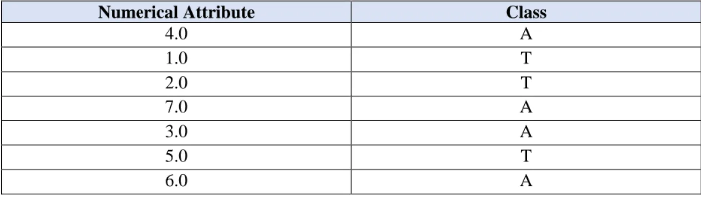
Table 1: An Example of a Univariate Decision Table

Numerical Attribute Class

4.0 A 1.0 T 2.0 T 7.0 A 3.0 A 5.0 T 6.0 A

Following the course of discretization, we sort the numerical attribute and pair the values together with their matched class labels, a list of ordered records is presented in Figure 1 as:

Since we are performing supervised discretization, sometimes the process is driven by the class labels, the candidate cut-points are 2.5, 4.5 and 5.5, where mid-values are adopted between those records with divergent class names. Each cut-point is evaluated using a particular criterion (e.g. information gain), and then the discretization procedures run recursively on both sides of the best cut-points until a stopping condition is met [12].

Compared to supervised discretization, unsupervised discretization is much simpler to comprehend and implement, which takes no account of class values while discretizing. However, this technique requires binning beforehand. Based on the way that bins (intervals) are defined, there are two main categories of studies (equal-interval and equal-frequency) in the literature of unsupervised discretization.

(1.0, T), (2.0, T), (3.0, A), (4.0, A), (5.0, T), (6.0, A), (7.0, A) ---↑---↑---↑---

2.5 4.5 5.5 Figure 1: An Example of Supervised Discretization

(13)

6

Equal-interval discretization, just as its name suggests, takes equal width over the whole range. For example, given a list of digital sequences (0, 1, 1, 5, 10, 20, 25, 30, 70, and 100) on behalf of a continuous feature. If we predefine five bins for this value range, each interval holds the value of 20, e.g. [0, 20), [20, 40), etc. Equal-interval discretization is displayed using an example, see Figure 2 in the below.

Figure 2: An Example of Equal-Interval Discretization

In this case, it is apparent that the value count within each bin is unequal, which is the principal defect of this method. Some bins are frequently invisible because there is no value distributed within its range, for instance, B3, which causes a certain amount of information loss. To overcome this, equal-frequency discretization introduces an alternative idea that sets an equal size to each bin.

An illustration of this method is provided in Figure 3, assuming five bins with equal frequency are applied to the same digital sequence above.

Figure 3: An Example of Equal-Frequency Discretization

The performance is manifestly enhanced to some extent, yet it is vulnerable to outliers because abnormal values can alter the ranges of intervals significantly [6].

0, 1, 1, 5, 10, 20, 25, 30, 70, 100 ---↑---↑---↑--- B1 B2 B4 B5 0, 1, 1, 5, 10, 20, 25, 30, 70, 100 ---↑----↑---↑---↑--- B1 B2 B3 B4 B5

(14)

7

Direct vs. incremental discretization

Direct discretization approaches are customarily guided by user’s pre-defined inputs, such as the number of intervals. All of the unsupervised discretization methods (e.g. Equal-Interval discretization, and K-means) fall into this category. In contrast, incremental discretization does not rely on precedent inputs. It initiates with an unpremeditated discretization practice, which is followed by constant refinements until a certain stopping criterion terminates the program [7].

Global vs. local discretization

The vital difference in this division of discretization approaches depends on whether the entire or partial feature space is considered. To be specific, global discretization evaluates all attributes before determining the cut-points for intervals. Local techniques only consider a restricted region of continuous features. They usually face the problem of determining how many intervals should be specified in terms of these numerical attributes, and this can occasionally jeopardize the entire course of discretization [8]. Even so, local discretization reveals a superior supervised classification rate when it jointly ties with the decision tree methods, such as C4.5, stated by Quinlan [20].

Static vs. dynamic discretization

This taxonomy depends on when discretization is conducted. Dynamic discretization proceeds simultaneously with the process of classification when a certain classifier is applied, which determines the optimal solution after evaluating the possibility for all attributes concurrently and considers the interdependency among them. Alternatively, static discretization is typically regarded as a preprocessing program, which only carried out an independent discretization on each

(15)

8

attribute, all unsupervised discretization methods that need pre-binning are part of this category. Further assessments between these two methods can be learned in [9].

Splitting (Top-down) vs. merging (bottom-up) discretization

Top-down discretization approaches start with no partitioning, they treat the whole continuous scale as one interval and gradually split into smaller ones until a certain stopping criterion is reached. Bottom-up approaches perform by maximizing the number of intervals and merge them progressively.

Also, there is a field of discretization study based on entropy measures that locally evaluate each of the potential cut-points to determine the boundaries for the intervals [16].

Suppose we are to evaluate all the candidate cut-points about the numerical attribute X with m

distinct values, and sorted as x1, x2, x3... xm. Each candidate cut-point of attribute X divides the entire data set into two regions or subsets. Suppose that p(x1), p(x2), p(x3)... p(xk) symbolize the probabilities for all k classes within either subset. The class entropy of a subset, denoted by E(R), is defined as follows [12]:

− ∑ 𝑝(𝑥_𝑖) × log₂𝑝(𝑥_𝑖) 𝑘

𝑖=1

Definition: For an attribute X of a data set with N samples, denoted by R, and a candidate cut-point

t, which divides R into two subsets 𝑅1 and 𝑅2, the entropy measure for attribute X, denoted by 𝐸(𝑋, 𝑡, 𝑅) and defined as follows:

|𝑅1|

𝑁 𝐸(𝑅1) + |𝑅2|

𝑁 𝐸(𝑅2)

(16)

9

The cut-point t with the minimal 𝐸(𝑋, 𝑡, 𝑅) is taken as the one that determines the optimal binary discretization on the attribute X. For example, let 𝐸(𝑋, 𝑡1, 𝑅) and 𝐸(𝑋, 𝑡2, 𝑅)be the class

information entropy based on the two possible cut-points t1 and t2 on attribute X. Then if

𝐸(𝑋, 𝑡1, 𝑅) > 𝐸(𝑋, 𝑡2, 𝑅)

we choose t1 as the best cut-point; otherwise, we partition based on t2 [8].

Some decision tree induction algorithms, such as ID3 with its extension (C4.5), use the information entropy in their algorithms. Gain theory is briefly discussed in the next section and further studies can also be referred to [12, 19].

2.2 C4.5 Learning Algorithm

C4.5, an extension of the ID3 learning algorithm, is a rule induction algorithm that can produce decision trees based on gain theory (discussed in the section 2.2.2). Both of these two algorithms were developed by Ross Quinlan in the 1980s.

2.2.1 Decision Tree

In data mining, a decision tree is a predictive model that represents treelike mapping relations between object properties (attributes) and object values (class labels). The structure of a decision tree be made up of elements that can be either a:

a) Leaf: a class label, or,

b) Non-leaf node: an attribute identity with branches (possible outcomes) which connect with subtrees [19].

Typically, a classification for a case using a decision tree starts from the root (top node) and traverses down to a leaf node that gives out the object value. While encountering a non-leaf node,

(17)

10

the traverse is shifted to one of the subtrees based on the outcome indicated by the specific observation of the case. In a decision tree, each path can represent multiple cases in a data set.

There are two principal types of decision trees in the literature:

a) Classification tree: its prediction results are discrete.

b) Regression tree: its prediction results are continuous values, for example, housing price. Compared to other classification algorithms in data mining, decision trees algorithms have some significant advantages:

a) Easy to read and implement.

b) Data preparations are simple or even unnecessary since other techniques usually require to normalize the data, such as removing redundancy or blanks.

c) Able to handle multiple data types (i.e. numerical, nominal). d) Able to keep feasibility and efficiency, even in a large data set.

Nevertheless, there is a severe deficiency in the entropy-based algorithms, such as ID3, since these algorithms tend to build the tree in favor of those attributes with more distinct values. Some paths in a decision tree occasionally characterize one or two cases; this will lead to a lot of subtrees. Even though it is a precise way to build the classification model, it extremely relies on the training data. The predicted accuracy rate will dramatically decrease as soon as a new unseen data is applied to the model, which is referred to as the issue of over-trained in machine learning. There are several approaches to prevent this problem during model construction; one practical way is to restrict the level of a decision tree to inhibit it from growing. Another approach is to set a minimum value that each node can represent, and it stops dividing when the number of records in the node are less than

(18)

11

this value. The C4.5 learning algorithm uses an alternative criterion called gain ratio that is discussed in the next section [19].

2.2.2 Information Gain and Gain Ratio

The entropy, which is used to evaluate the candidate cut-points and its definition is introduced while we discuss discretization in the section 2.1. In this section, we present another related concept, called information gain, which is the complement of entropy measures and evaluate the certainty of the information content. All the following definitions can be found in Quinlan’s book [19].

Let there are n possible outcomes that partition a set of training samples T on an attribute X into subsets T1, T2 … Tn. Let Ti denotes one of these subsets, 𝑓𝑟𝑒𝑞(𝐶𝑗, 𝑇𝑖) indicates the number of

samples in 𝑇𝑖 with the class label 𝐶𝑗 (suppose that there are totally k class in 𝑇𝑖, and |𝑇𝑖| denotes

the number of samples in the subset Ti).

So the information conveyed from the subset Ti with the unit of bits, indicated by 𝑖𝑛𝑓𝑜(𝑇_𝑖), which is also known as the information entropy, can be calculated as follows:

− ∑𝑓𝑟𝑒𝑞(𝐶𝑗, 𝑇𝑖) |𝑇_𝑖| × log2( 𝑓𝑟𝑒𝑞(𝐶𝑗, 𝑇𝑖) |𝑇_𝑖| ) 𝑏𝑖𝑡𝑠 𝑘 𝑗=1

Since there are n possible outcomes in terms of the attribute X, the overall conveyable information is the weighted sum over the whole outcomes, denoted by 𝑖𝑛𝑓𝑜_𝑋(𝑇) and defined as follows:

∑|𝑇𝑖|

|𝑇|× 𝑖𝑛𝑓𝑜(𝑇𝑖) 𝑛

𝑖=1

(19)

12

Therefore, the information gain of the attribute X, denoted by 𝑖𝑛𝑓𝑜𝐺𝑎𝑖𝑛(𝑋)and defined as follows:

𝑖𝑛𝑓𝑜𝐺𝑎𝑖𝑛(𝑋) = 𝑖𝑛𝑓𝑜(𝑇) − 𝑖𝑛𝑓𝑜_𝑋(𝑇)

𝑖𝑛𝑓𝑜(𝑇) denotes the average information entropy, which is also an entropy-based measure on the class attribute.

An example based on the information gain criterion test is given underneath, see Table 2 below.

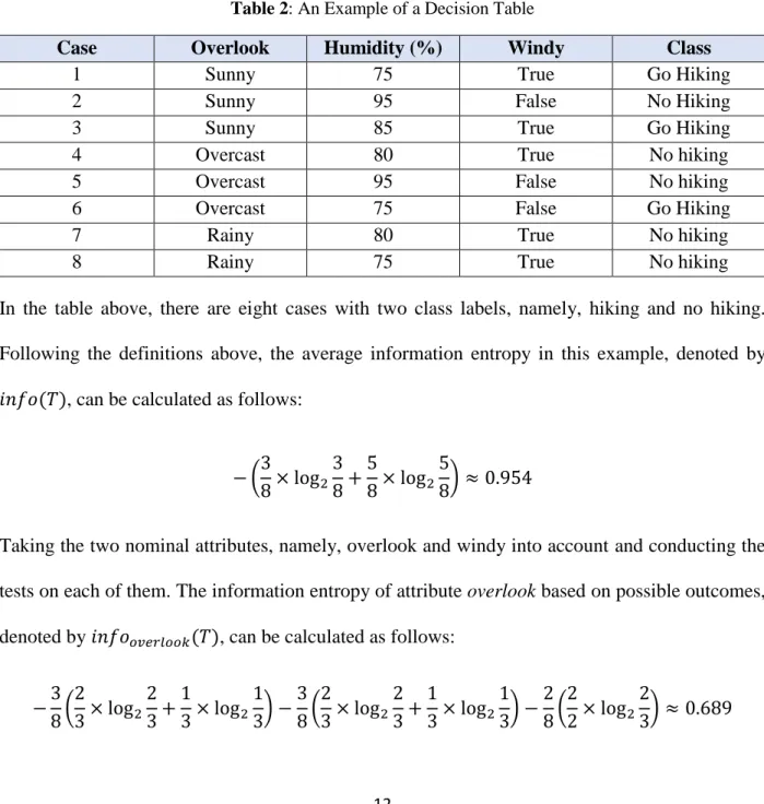
Table 2: An Example of a Decision Table

Case Overlook Humidity (%) Windy Class

1 Sunny 75 True Go Hiking

2 Sunny 95 False No Hiking

3 Sunny 85 True Go Hiking

4 Overcast 80 True No hiking

5 Overcast 95 False No hiking

6 Overcast 75 False Go Hiking

7 Rainy 80 True No hiking

8 Rainy 75 True No hiking

In the table above, there are eight cases with two class labels, namely, hiking and no hiking. Following the definitions above, the average information entropy in this example, denoted by

𝑖𝑛𝑓𝑜(𝑇), can be calculated as follows:

− (3 8× log2 3 8+ 5 8× log2 5 8) ≈ 0.954

Taking the two nominal attributes, namely, overlook and windy into account and conducting the tests on each of them. The information entropy of attribute overlook based on possible outcomes, denoted by 𝑖𝑛𝑓𝑜_{𝑜𝑣𝑒𝑟𝑙𝑜𝑜𝑘}(𝑇), can be calculated as follows:

−3 8( 2 3× log2 2 3+ 1 3× log2 1 3) − 3 8( 2 3× log2 2 3+ 1 3× log2 1 3) − 2 8( 2 2× log2 2 3) ≈ 0.689

(20)

13

Hence the information gain about the attribute overlook can be calculated as follows:

𝑖𝑛𝑓𝑜𝐺𝑎𝑖𝑛(𝑜𝑣𝑒𝑟𝑙𝑜𝑜𝑘) = 0.954 − 0.689 = 0.265

The similar computations in terms of attribute windy is shown as follows:

𝑖𝑛𝑓𝑜𝑤𝑖𝑛𝑑𝑦(𝑇) = − 5 8( 3 5× log2 3 5+ 2 5× log2 2 5) − 3 8( 2 3× log2 2 3+ 1 3× log2 1 3) ≈ 0.951 𝑖𝑛𝑓𝑜𝐺𝑎𝑖𝑛(𝑤𝑖𝑛𝑑𝑦) = 0.954 − 0.951 = 0.003

In gain theory, the attribute that maximize the information gain is selected as the optimal node for splitting. With the information gain of 0.265, the attribute overlook is chosen as the top node (or root) of the tree (if numerical attribute humidity is ignored).

However, as mentioned at the end of last section, entropy-based methods make the tree model too “leafy” since gain theory tend to pick the attribute with many distinct values but sometimes not quite relevant. To overcome this, C4.5 learning algorithm adopts another criterion, termed as gain ratio, to handle attribute selection. This rule is based on information gain and an additional concept called split information. The following formula represents the splitting information about attribute

X, denoted by 𝑖𝑛𝑓𝑜𝑆𝑝𝑙𝑖𝑡(𝑋): − ∑|𝑇𝑖| |𝑇| 𝑛 𝑖=1 × log2 |𝑇_𝑖| |𝑇|

where the symbols in the above equation hold the same meanings as in the discussion of information gain as described above [19].

(21)

14

𝑖𝑛𝑓𝑜𝐺𝑎𝑖𝑛(𝑋) 𝑖𝑛𝑓𝑜𝑆𝑝𝑙𝑖𝑡(𝑋)

With the support of split information, the C4.5 learning algorithm can build models in a much more efficient manner. The splitting information increases if the target attribute is too informative (with plenty of distinct values). Relatively, this can adjust the gain ratio for each attribute when there is a need to rank them, indicating that the C4.5 learning algorithm can potentially dispose of the side effects of information gain. Apparently, balanced attributes (with a reasonable amount of distinct values but more relevant) will be ranked to be higher in gain ratio theory.

Likewise, the gain ratio criterion selects the attribute that maximizes the outcome, but two presumptions are required to be written down beforehand according to [19]:

a) The information gain about the chosen attribute should be large enough, at least larger than the average information gain value over all the attribute tests.

b) The number of training cases in the data set should be far greater than the number of classes.

Compare to information gain, gain ratio is an even more effective criterion. Moreover, the performance is much more satisfactory when each attribute test is binary in the course of building a decision tree model according to Quinlan’s experiments demonstrated in [19].

Still, there are some downsides if gain ratio is adopted to determine the cut-point value of a numerical property. For example, according to the formula above, it is manifest that the gain ratio is maximized when a cut-point divides the data set into two equal parts with the same number of samples within either subset. It is unreasonable and even inhibited that the number of samples in a subset can affect the decision of picking the demarcation point. On the other hand, suppose that information gain is adopted to determine the selection of attributes, the decision tree will eventually turn out to be too “luxuriant”. The main reason is that information gain measurement

(22)

15

prefer to choose those attributes with more different values and lack of ways to prevent the tree from germinating. Therefore, in C4.5, Quinlan indicated that there is a need to use information gain as the indicator to determine the cut-off points for numerical attributes, while to use gain ratio as the indicator to decide attribute selections [19].

2.2.3 Possible Attribute Tests in C4.5

Some possible tests to find the best candidate attribute in C4.5 include:

a) Discrete attribute test: each value of a discrete attribute leads to an outcome that produces a branch.

b) Continuous attribute test: typically, a threshold K is defined to divide the sequence of the continuous values within a numerical attribute, denoted by A, into two binary parts (A≤K and A>K), representing smaller than or equal to and larger than [19].

2.2.4 Handling Continuous Features in C4.5

As mentioned in the previous section, the C4.5 learning algorithm handles numerical attributes by discretizing the continuous scale into two intervals. But it is hard to express precisely the test in a continuous sequence since there are countless possibilities to set the thresholds. In C4.5, the selections of thresholds are manipulated in such a way that the optimal threshold will be captured. In a usual way, the averages of two adjacent distinct values are put into a threshold pool for evaluation after sorting. The evaluation tests are conducted on every threshold.

For instance, a training set holds a numerical attribute with a finite number of values in the ordinal sequence as {v1, v2 … vk}, so the maximal number of candidate thresholds is k-1. One possible threshold divides the sequence into two partitions, denoted by {v1, v2 … vi} and {vi+1 … vk}, which give out the value of the threshold as follows:

(23)

16

𝑣_𝑖 + 𝑣_𝑖+1 2

It might be lavish to test all these thresholds; however, when the cases are sorted, the process should be carried out effortlessly. According to Quinlan’s book [19], in order to make sure that the thresholds are the actual values from the training set, the largest attribute values that do not exceed each of possible midpoint values are picked as the thresholds. To demonstrate this, we take the numerical attribute humidity from Table 2 as an example, the possible thresholds with the actual thresholds given in the subsequent bracket, are shown in the Figure 4.

Figure 4: Possible and Actual Thresholds of a Sorted Sequence in C4.5

As a conclusion, the C4.5 learning algorithm generates a decision tree based on comparing the test results over all attributes based on information gain or gain ratio criterion. Discrete-value attributes can be directly tested, while continuous-value attributes are required to be tested based on each candidate cut-off point.

2.2.5 Pruning the Tree

Generating a decision tree in a greedy way by evaluating every candidate cut-point can be extraordinarily sophisticated, which can make it possible that the training samples covered by the tree nodes are almost “pure”. Therefore, to a great extent, such decision trees can adjust to training sets properly and present good classification performances with low error rates. However, the outliers in a training set can also be learned by a decision tree and become parts of it. Once the tree model is applied to an independent test set, the performance of classification turns out to be worse

75 75 75 | 80 80 | 85 | 95 95 ---↓---↓---↓--- 77.5(75) 82.5(80) 90(85)

(24)

17

which is called overfitting problem. Quinlan pointed out that the predicted error rate about a test set appears to be higher based on a full-grown tree comparing to using the pruned one [19].

There are two families of pruning approaches: Pre-pruning and Post-pruning.

Pre-pruning: stop the growth of a decision tree during the modeling process. To control this, we need to set a condition that is also called the stopping criterion. There are several possible criteria provided in the below:

a) When all of the samples in the subtree belong to the same class. b) When the maximal tree depth is reached.

c) When the number of samples covered by the subtree is less than a threshold or a certain proportion.

d) The optimal partitioning (split) gain is less than a certain threshold, such as the error value etc.

Post-Pruning: the pruning procedure is conducted on a fully generated decision tree. Some methods in this category contain:

Reduced-error pruning (REP)

This pruning method considers each non-leaf node of the tree as a candidate for pruning, and the trimming process on a candidate node has the following steps:

a) Remove the subtree which is derived by this node. b) Make it as a leaf node.

c) Assign the most common class among all the training samples covered by the subtree of this node.

(25)

18

d) Validate whether there is an improvement in terms of performance (predicted error rate on a test set).

Due to overfitting, it can be essential to make a validation (test) set, iteratively repeat the operation above to verify the node from the bottom up, and delete those nodes that diminish the accuracy rate.

REP is one of the easiest post-pruning methods whose drawbacks become even critical when the data is scarce since characteristics in a small-scale training set are ignored in the pruning process. Despite that, this method is still used as a benchmark to evaluate the performance of other pruning algorithms.

Pessimistic Error Pruning (PEP)

The C4.5 learning algorithm uses another pruning approach called PEP originated from the post-pruning family. The fundamental idea of pessimistic post-pruning approach in the C4.5 learning algorithm is to evaluate recursively the predicted error rate using test samples upon each internal node. There is no essential difference between PEP and other techniques in terms of the pruning process, which can be briefly described as: each non-leaf node is trimmed as a leaf node whose class identity is determined by the most “voted” label of samples covered the original subtree, followed by comparing the predicted error rate before and after pruning to decide whether or not to prune. The only difference depends on how to evaluate the predicted error.

There is no doubt that the predicted error rate will arise if we replace a subtree (multiple leaf nodes) with a particular leaf node, but unnecessarily on a yet-unseen data. So we need to add an empirical penalty factor in terms of the calculations of the error rates [19].

(26)

19

Suppose that there are N samples that are covered by a leaf node and part of them are misclassified, say the number is K. Naively, the error rate is K/N which demonstrates the possibility of the predicted error. The difference is that, in PEP, the probability of error rate of this leaf node can be calculated as (𝐾 + 0.5)/𝑁. The 0.5 here is the penalty factor, also called significance level. Similarly, assume that there are L leaf nodes in a subtree; thus the probability of predicted error rate of the subtree can be calculated as follows:

∑ 𝐾_𝑖+ 0.5 × 𝐿 ∑ 𝑁𝑖

where K and N_i _i respectively represent the misclassified and the total number of samples covered by the ith_{leaf node in the subtree.}

This probability is empirically evaluated to be numerous distribution models, such as binomial distribution or Gaussian distribution. We use the upper limit of this probability as the criterion to make the pruning decisions, written as 𝑈_𝐶𝐹(𝐾, 𝑁). Two additional regulations of the probability calculations are given as follows:

a) The predicted error rate of the original subtree is the sum of associated error rate of each branch.

b) Assuming a leaf node covers N cases with K misclassifications; thus the predicted error of this leaf node can be written as 𝑁 × 𝑈_𝐶𝐹(𝐾, 𝑁) [19].

Currently, the PEP approach is categorized to be one of the post-pruning algorithms with the highest precision, but still flawed. It is primarily used only for top-down pruning strategy that leads to the same problem as pre-pruning approaches that occasionally prune some unnecessary child nodes. Besides, this method most likely results in a failure during the process.

(27)

20

Although the pessimistic method has several limitations, it still exhibits accepted results in practice. Moreover, PEP method no longer requires separate training sets and validation machines which are favorable to small data sets. Beyond that, compared to other pruning methods, its strategy is much more efficient and faster since every single subtree is visited once during the practice. In a worst case, its computation time complexity yields a linear relationship with the non-leaf node in the unpruned original tree [23]. An example of PEP method used by the C4.5 algorithm is provided to demonstrate how it works.

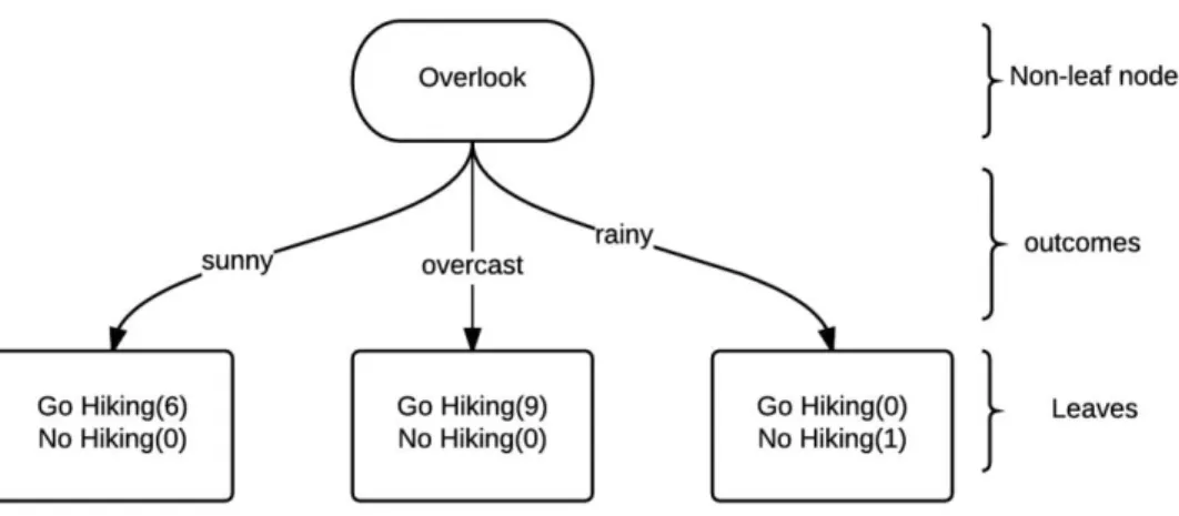
Given a training set of 16 cases, an unpruned subtree with three possible outcomes in terms of the attribute overlook covers all these cases with no misclassification. The number in the bracket represents the number of samples covered by the leaf node. See Figure 5.

Figure 5: An Example of an Unpruned Subtree

Before pruning, the predicted error rate of the unpruned subtree is the weighted sum upon each branch, and it can be derived from the procedures as follows:

For the first leaf node, N = 6 and K = 0. Using the default significance level of 0.25 in the C4.5 learning algorithm, we have 𝑈_0.25(0,6) = 0.206, so the predicted error rate for the first leaf node

(28)

21

is 6 × 0.206. Apply the same to the second and the third leaf node, we have 𝑈_0.25(0,9) = 0.143 and 𝑈0.25(0,1) = 0.750. Thus the predicted error rate for this unpruned subtree is the sum of error

rate on each leaf node, which can be calculated as:

6 × 0.206 + 9 × 0.143 + 1 × 0.750 = 3.273

If the subtree is replaced by a leaf node with the class label called Go Hiking, it covers the same 16 cases with one case that is misclassified. So the predicted error for the leaf node after pruning is:

16 × 𝑈_0.25(1,16) = 2.512

which is smaller than the previous unpruned error rate.

Hence the decision is made; the original subtree is considered to be pruned into a leaf node by using PEP method [19].

2.2.6 Soft Thresholds

If there are missing values within a discrete attribute, a probabilistic measure over all possible outcomes, can be assigned to them to supply a quantitative analysis.

As discussed in the previous sections, the values of a continuous attribute are handled by placing them into two unengaged ranges, which potentially transforms a continuous attribute into a binary one with probability. Roughly, the probability of the numerical value is determined by the proportion of the range that lies in one side of the threshold. For example, given a threshold Z with the value of 6, and a numerical attribute A with the value range from 4 to 12, so the probability for A≤Z denotes 0.25, which can be calculated as:

6 − 4 12 − 4

(29)

22

Each numerical value is compared against the threshold and clustered into one of the two partitions. If an enormous gap exists between an attribute value and the threshold, there is no doubt that a case with this value will be sent along the path and unmistakably lies on one side of a subtree. However, if the value stands too close to the threshold, once the value is made with a minor change due to misoperations, it will lead to a radically different classification [19].

Carter and Catlett introduced a concept called “soften” thresholds in [5], and defined two relative thresholds, which are two new values close to the original threshold Z, denoted by below (Z-) and above (Z+). If we have a case value V for a continuous attribute A, so the probability of A≤Z, denoted by 𝑃(𝑉), can be defined as follows:

a) If V is less than Z-, 𝑃(𝑉) is equal to 1.

b) If V lies between Z- and Z, 𝑃(𝑉) can be interpolated between 1 and 0.5. c) If V lies between Z and Z+, 𝑃(𝑉) can be interpolated between 0.5 and 0. d) If V is larger than Z+, 𝑃(𝑉) is equal to 0.

Take the complementary probability for the outcome A>Z and follow the similar patterns in the definition above [19].

The new threshold is chosen to set to either Z- or Z+ based on the misclassification. Suppose that the number of misclassifications associated with the original threshold denotes K, the new threshold might set to either of these two soft thresholds if either one of them yields the number of misclassification that is one standard deviation more than K in the current test. The standard deviation of number of misclassifications can be defined as [19]:

√(𝐾 + 0.5) × (|𝑁| − 𝐾 − 0.5)/|𝑁|

(30)

23 2.3 Random Forests Learning Algorithm

Decision tree induction algorithms, such as ID3 and C4.5, are effective approaches to building models with low complexity and intuitionistic exhibition in the literature with many advantages over other classification algorithms such as logistic regression and SVMs. Also, they can generate models with extremely high accuracy rates on training sets, but the generalization error on unseen data is commonly unsatisfied due to the over-adaptation on the training sets.

Due to the C4.5 learning algorithm, conducting pruning on a fully-built tree can alleviate the overfitting problem, but does so at the expense of the accuracy of the original model. Hence there is a thoughtful issue of trade-off while constructing a single decision tree, and this trade-off is sometimes arbitrary and hard to handle. Nonetheless, Ho pointed out that these difficulties are not rooted in the tree classifiers intrinsically, which means there is a way to optimize the generalization error on unseen data as well as to keep the accuracy of the training model [13].

Random forests algorithm, is an extended learning approach based on the thought of gathering a multitude of decision trees [24]. The algorithm that induces a random forest was first developed by Leo Breiman [4]. The essence of random forests learning is to generate a forest that is composed by multiple decision trees in a random way. Each spanning tree in the forest independently determines the class label of an input vector (record), and the final decision for the record is made with the most chosen category over all the independent decision trees in the forest. This approach, first propounded by Ho, combines the idea of tree bagging and the randomized subspace of the attributes for building a single tree [13, 14]. Similar to the C4.5, random forests can also handle both discrete and continuous properties. In addition, it can also be used for unsupervised learning and outlier detection. The generalization error of the model generated by using random forests induction algorithm depends on the strengths of single trees and the correlations among them.

(31)

24 2.3.1 Advantages of Random Forests

Random forests are robust against missing data and unbalance data, and it is well known as one of the best classification algorithms in machine learning [4]. Advantages of random forests algorithm are concluded in the contents below:

a) Fast-speed learning and prediction, it can produce a good performance even in a data set with numerous classes.

b) Provides an effective method with fault-tolerant capability which is robust against rough sets with outliers and noises. Maintains a high precision even when aim at learning a data set with a large proportion of missing data [4].

c) Handles high-dimensional data without a need for feature selection or pruning.

d) Generates an unbiased estimate of the generalization error in the classification process. e) Detects the degrees of feature correlations, internal strengths and variable importance. f) No overfitting problem.

g) Easy to achieve and implement.

2.3.2 Construction of the Forest

Random forests induction algorithm is primarily applied to regression (not discussed here) and classification problems and it borrows general thought of bagging (one resampling technique) and expand it to double levels of randomness, namely tree bagging and feature bagging. Tree bagging, also named bootstrap aggregation, is an ensemble method that combine tree algorithm and other classifiers in machine learning. The method repetitively selects random samples from the original training set and form a new training set with the same size. It is a refundable process which means it will replace the original “bag” after every fetch. The new set contains replicates, and there is no

(32)

25

possibility for the new set to be identical to the original training set once the size of the set is sufficiently large [24].

Given a training set with n samples X = x1, x2, …, xn with its corresponding class Y = y1, y2, …, yn. In tree bagging, it repeatedly selects n random samples with replicates from the training set (X, Y) and construct a decision tree model that fits this new set. Suppose that we need to build B number of trees in a forest, the construction of the forest using the idea of tree bagging is given as follows [24]:

For b = 1, 2, …, B:

1. Select a set of n random samples from X, Y, and form a new training set, denoted by (Xb,

Yb).

2. Construct a classification tree Tb, which fits the set (Xb, Yb).

The prediction error for unseen samples can be evaluated on each tree Tb after the model is established, where the most popular “vote” among all the decision trees in the forest is assigned to the unseen samples. Bagging is an effective way to reduce the generalization error since it is able to minimize the variance of the model [24]. Although a single model is sensitive to noise, analyzing multiple trees can exclude the interventions as long as the obtained trees themselves are not associated [2]. Even if tree bagging enhances the bias to a degree, it is sure that the generalization error decreases using this technique.

There is another key difference that distinguishes the bagging mechanism used by random forests from the original bagging algorithm. That is; random forests use a modified decision tree learning algorithm which generates each independent decision tree based on a randomized subset of not only the samples but the features; the process is usually called feature bagging. The intention of

(33)

26

conducting two dimensions of bagging, on the basis of rows and columns separately, mainly attribute to reducing the correlations among independent decision trees in the forest. Supposing some attributes of the training set are dominant predictors for target outputs, most of the independent decision trees incline to “embracing” these attributes in the building course, which will result in an unanticipated problem that the obtained decision trees are probably correlated to each other [24]. Besides, two phases of bagging exhibit several benefits because they provide an ongoing and internal error estimates of some parameters of the classification accuracy, such as generalization error of the ensemble of trees, strengths etc [4].

As an ensemble learning, random forests combine multiple deep learned models (decision trees) with high variance but low bias together and take the average of the complex fit trees. It also uses two levels of “bagging” to learn every different part of the training set to control the variance. The bias will slightly increase, but it provides an optimal solution that minimize the generalization error and benefits the entire model [24].

In the establishment of a single decision tree, random forests learning algorithm uses the C&RT learning algorithm which adopts Gini coefficient as the impurity-based measures to select variables. The definitions of C&RT and Gini coefficient can be referred in the section 2.3.4 below. We provide the pseudo-code of the learning process of a single unpruned decision tree based on the Gini coefficient in Appendix A, which can be referred to in [4].

2.3.3 Out-Of-Bag Error Estimates

In random forests learning algorithm, there is no need to set manually aside a part of the samples as a test set to obtain an unbiased error estimate. The estimations are conducted internally in each process. Briefly speaking, one-third of the samples are left out as a remaining part in the course of bootstrapping (tree bagging). Suppose that m trees are estimated, each case in the remaining part

(34)

27

is taken down to each tree in the forest and obtains approximately m/3 number of class votes. The most popular vote is assigned to the case. The proportion of cases in the remaining part with the votes that are not equal to the original class label are called the out-of-bag error estimate. This error estimate decreases as the number of tree classifiers in the forest increases. The estimated results are proved to be unbiased and as accurate as using a test set with the same size of the training set [3, 4]. Moreover, strength and correlation, two vital parameters which are associated with the accuracy of an individual classifier, can be estimated by the out-of-bag approach. Clearly, an ideal solution is to reduce the correlations among the classifiers and maintain high strengths. Further discussion of estimations of strength and correlation can be found in [4].

2.3.4 C&RT Algorithm and Gini Gain

C&RT, short for Classification and Regression Tree, is a recursive partitioning algorithm to build classification and regression trees for machine learning, which was first popularized by Breiman et al. in [1]. Different from ID3, C&RT algorithm uses a different splitting criterion, called the

Gini coefficient or Gini index, to determine the ideal attribute for splitting while learning the tree model. Similar to entropy measure, the Gini coefficient is also an impurity-based criterion that is able to measure the deviations within the probability distribution of the target attribute’s values [21], and the result becomes larger if there are additional different clusters in the distribution. Suppose that there are m different classes {1, 2 … m} in a partition with each of the corresponding probability called fi. The Gini coefficient of this partition, denoted by 𝐼𝐺(𝑓) and calculated as:

∑ 𝑓𝑖(1 − 𝑓𝑖) = 1 − ∑ 𝑓𝑖2 𝑚

𝑖=1 𝑚

𝑖=1

Similar to information gain, Gini gain on the target attribute X, denoted by 𝐺𝑖𝑛𝑖𝐺𝑎𝑖𝑛(𝑋), can be defined as follows:

(35)

28

𝐼_𝑎𝑣𝑔(𝑓) − ∑|𝐺𝑖|

|𝐺| × 𝐼𝑖(𝑓)

where 𝐼_𝑎𝑣𝑔(𝑓) indicates the average Gini coefficient that is evaluated on the class attribute, |Gi| represents the size of the ith partition [1].

The best attribute for splitting is the one with the maximized Gini gain. Since trees built by C&RT method are all binary ones, both discrete attributes and continuous attributes should be divided into two binary substitutes based on threshold values, and the process can be evaluated by Gini gain. It is analogous to the way of numerical processing in the C4.5 learning algorithm which is already discussed (can be referred to section 2.2.4).

(36)

29

Chapter 3 Research Methodology

The method we proposed in this thesis is a global discretization algorithm that disposes continuous attributes as preprocessing in machine learning. Specifically, we discretized all numerical attributes within the original data set and replaced each of them with multiple nominal ones based on all potential cut-points. A discretized data set, which only includes categorical attributes, is obtained by applying our preprocessing method. We carried out two groups of experiments on both data sets (original and discretized data sets) by separately using two decision tree learning algorithms, namely C4.5 and random forests, to each of them. After this procedure, we evaluated the performances (prediction accuracy rate) of every decision tree model using the technique called cross-validation. Both of the above experimental phases were accomplished in Weka software. Once the experimental data were thoroughly obtained, two Wilcoxon tests were performed in terms of isolated classifiers, each of which were conducted to compare whether there is a level of statistical significance between two populations (the original and discretized data set). Twelve pairs of data sets were applied to the experiments. See the content below for in-depth descriptions of our preprocessing approach.

3.1 Descriptions of ARFF Data File

All the original data sets were acquired from the U.C. Irvine repository (UCI) for experimental use [18]. Each complete (with no missing value) data set contains at least one numerical attribute and ends with the suffix of .arff.

ARFF is short for Attribute-Relation File Format. It is the default file format that can be recognized or generated by Weka machine learning software [22].

(37)

30

ARFF consists of two sections, namely Header and Data. A typical ARFF file begins with some comments identifying by using symbol % as the first character of each line, followed by the name of the relation which is labeled by @relation in the header. Another block of the header is the attribute part. This block is composed by the labels @attribute and the name of the attributes with their types. We provide an example of the header from an ARFF file named cmc.arff. In order to quote the information for explanation, we also provide the origin, creator of the data set and the date when it was generated, see Figure 6 below.

Figure 6: ARFF Header Section

As shown in the illustration above, the name of the relation is cmc, and seven features with a class attribute are described in the header, most of them are nominal ones.

Generally, there are several fixed types that can be identified by Weka software. % 1. Title: Contraceptive Method Choice

%

% 2. Sources:

% (a) Origin: This data set is a subset of the 1987 National Indonesia % Contraceptive Prevalence Survey

% (b) Creator: Tjen-Sien Lim ([email protected]) % (c) Donor: Tjen-Sien Lim ([email protected]) % (c) Date: June 7, 1997

%

@relation cmc

@attribute Wifes_age numeric @attribute Wifes_education {1,2,3,4} @attribute Husbands_education {1,2,3,4}

@attribute Number_of_children_ever_born integer @attribute Wifes_religion {0,1}

@attribute Wifes_now_working? {0,1} @attribute Media_exposure {0,1} @attribute class {1,2,3}

(38)

31

a) Numeric: defined by the keyword numeric which can also be replaced by integer or real, such as Wifes_age and Number_of_children_ever_born in the example above.

b) Nominal: defined by a list of possible values in a curly brace representing the type of an attribute. For example, type { 1,2,3,4 } for nominal attribute Wifes_education. It is noteworthy that the class attribute is a special nominal one. It is normally introduced by the keyword class and indistinguishable from other nominal attributes, which means ARFF data file does not specify which attribute is allocated to be the predicted one [22]. This setting gives a huge flexibility for data learning using Weka software.

c) String: identified by the keyword string, and strings are some textural values highlighted by the quotation mark. String type is very advantageous especially in text mining and can be put into use with some unsupervised filters in Weka software, such as StringToNominal

and StringToWordVector.

d) Date: a particular string with the format of yyyy-MM-dd-THH:mm:ss (4-digits year, 2-digit month, 2-digit date and time), for example, 2015-04-03T12:16:00. Although it is identified as a string attribute, it is converted into a numerical value when it need to be treated as an operand.

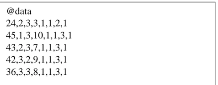
Following the section on attributes, it comes to the data interpretation which starts with the keyword @data. Each case is displayed in one line with values following the order of the attributes which is described in the header, and the values are separated by commas. Missing values are indicated by questions marks. The following is the data section with five cases which is also from data file cmc.arff. See Figure 7 on the next page.

(39)

32

Figure 7: ARFF Data Section

More information about the format of ARFF file can be referred to [22].

3.2 Discretization Method as Preprocessing

As described in chapter two, both C4.5 and random forests learning algorithms are only able to construct the decision tree models based on categorical properties, consequently, numerical attributes in a data set should be completely transformed into discrete ones by conducting the technique of internal discretization during the process of learning the model. The method we proposed makes changes to the procedures above and handle continuous attributes as preprocessing before applying the induction algorithms to the data sets.

The following flowchart gives an overview of how a discretized data set is obtained using our preprocessing method based on the original data set, see Figure 8 on the next page.

@data 24,2,3,3,1,1,2,1 45,1,3,10,1,1,3,1 43,2,3,7,1,1,3,1 42,3,2,9,1,1,3,1 36,3,3,8,1,1,3,1

(40)

33

Figure 8: An Overview of Our Discretization Method

It is an unsupervised global discretization algorithm which takes all the candidate cut-points (thresholds) within every numerical attribute into account. See the descriptions below.

Algorithm: Let { A1, A2, …, Ai, Ai+1, Ai+2, …, An } be the set of attributes in a data set, where A1,

A2, …, Ai are continuous and Ai+1, Ai+2, … An are discrete (0 < i ≤ n). Let { Ci,1, Ci,2, …, Ci,j } be the set of potential cut-points within the ith continuous attribute Ai (each cut-point is the average of two consecutive values), we define our preprocessing method as follows:

For each continuous attribute Ai, where i = 1, 2,…:

A set of j number of discrete attributes are generated and to replace the ith continuous attribute Aiin terms of each candidate cut-point Ci,j(0 < i ≤ n), denoted by { Ai,1, Ai,2, …,

(41)

34

Ai,j }, each of which holds two discrete values representing larger than and smaller than, denoted by >Ci,jand <Ci,j.

The discretized data set contains both newly generated discrete attributes and the discrete attributes inherited from the original data set, denoted by { A1,1, A1,2, …, Ai,1, Ai,2, …, Ai,j, Ai+1, Ai+2, … An}. Suppose that there are three numerical attributes in a data set with three, four and five distinct values respectively within each of them. Rather than to find the best cut-point, we consider all candidate cut-points within each attribute, which is the averages of consecutive numerical values. Therefore, there are nine (2 for the first numerical attribute, 3 for the second and 4 for the third) candidate cut-points waiting for consideration.

According to the algorithmic descriptions above, for each candidate cut-point, we create a new nominal attribute with two discrete categories (symbolic values). For example, given a numerical attribute age with a candidate cut-point, such as 22. A new discrete attribute, namely age_22, will be generated with two discretized values (<22 and >22). As for another example, a list of 6 numerical values (within the numerical attribute age mentioned above) are sorted as 20, 20, 24, 24, 32, and 46, so the candidate cut-points are 22, 28, and 39. Based the algorithm, three nominal attributes are created, namely age_22, age_28 and age_39, each of which holds two categorical values labeling person as “older than” or “younger than” in this case. By comparing the actual target attribute’s value against the cut-point value, the case value of the newly introduced attribute can be filled with one of the two categories.

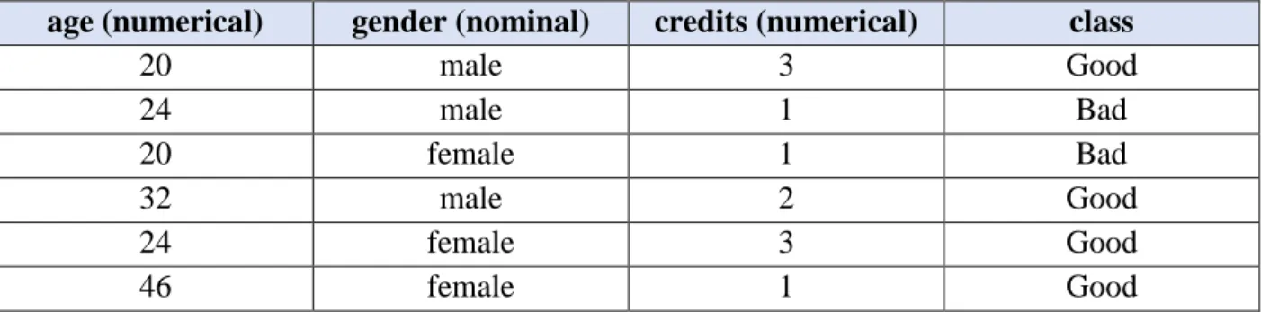
A comprehensive example which simulates our discretization method. We provided eight cases with four attributes, and the contents are shown in the Table 3 on the next page.

(42)

35

Table 3: An Example of a Data Set with Numerical Attributes

age (numerical) gender (nominal) credits (numerical) class

20 male 3 Good 24 male 1 Bad 20 female 1 Bad 32 male 2 Good 24 female 3 Good 46 female 1 Good

Throughout the entire table above, two numerical attributes are included in this data set, namely

age (4 distinct values) and credits (3 distinct values). After sorting, we have three candidate cut-points (22, 28, and 39) for the attribute age and two (1.5 and 2.5) for credits. According to our method described above, five nominal attributes are generated and taken to substitute for the original two numerical ones (age and credits). The discretized data set with modified format is provided in Table 4 below.

Table 4: The Discretized Data Set

age_22 age_28 age_39 credits_1.5 credits_2.5 gender class <22 <28 <39 >1.5 >2.5 male Good >22 <28 <39 <1.5 <2.5 male Bad <22 <28 <39 <1.5 <2.5 female Bad >22 >28 <39 >1.5 <2.5 male Good >22 <28 <39 >1.5 >2.5 female Good >22 >28 >39 <1.5 <2.5 female Good The purpose of discretization is to adjust numerous digital values into an interval, and information loss is inevitable since a considerable number of different values will be brought into a cluster. Keeping a close-up view of Table 4, the discretization method we presented is able to hold the internal information within the original digital numbers by projecting them into a two-dimensional space with candidate cut-point as one dimension and the binary values as the other one. Therefore, the consistency of the discretized data set maintain at the same level as the original one. If we

(43)

36

assemble those associated attributes in the discretized data set and test their consistency, there is no doubt that they perform as the digital values in the original data set. For instance, if we group the first three associated attributes in Table 4 and evaluate them on the row basis, case 1 and case 3, case 2 and case 5 are the same, all of which are different from either case 4 or case 6. Obviously, it performs the same patterns as the original data set. Although the method can preserve the original information within each numerical attribute, the expansion of attributes in some data sets can be extremely huge (refer to Table 5 and Figure 10), which might lead to a risk of overfitting. However, both C4.5 and random forests handle continuous attributes within the original data sets in a greedy way that evaluate every potential cut-point based on a certain criterion (described in 2.2.4 & 2.3.4). In contrast, when applying the discretized data sets to both classifiers, the procedures of internal discretization are skipped since all the numerical values are preprocessed. Beyond all doubt, both data sets produce the same time complexity to build the decision trees, even if the size of the discretized data sets are much larger compared to its original pair.

3.3 Classification and Evaluation Processes

Both decision tree learning algorithms (C4.5 and Random forests) are applied to the original and discretized data sets. We use Weka software which provides a good support for multiple machine learning algorithms to carry out the processes of learning the models and performance evaluations. The flow chart in the below gives a sketch for the procedures of the experiments based on classifier C4.5, see Figure 9 on the next page.

(44)

37

Figure 9: A Flowchart for the Experimental Procedures based on C4.5 Classifier

As described in chapter two, learning the models and making predictions based on the identical data population are meaningless and would fail to predict anything valuable on unseen data which surely lead to overfitting problem. One solution is to manually separate a data file into a training set and a test set. Build the model with the training part and then apply the obtained model on the test set to evaluate the performances. Even so, a risk of overfitting on the unseen test samples still exists, since the patterns in the test set might “leak” into the trained model while we are tuning the parameters of the estimator and the estimation would not exhibit a generalization performance of the model [15].

By introducing a validation set, an independent data set is divide into three parts. Model building and validation are carried on the training set and validation set separately. When the experiment comes to a success, an isolated test set is used for evaluation. However, the drawback of this technique is that the number of samples for learning the model are dramatically distributed.

(45)

38

Cross-validation (CV) is an estimation method which can balance both of the problem mentioned above. In this technique, the validation data set is no longer needed. The estimation method we used for our experiments is called k-fold CV. Essentially, an independent date set are randomly divided into k equal parts or folds, the model is built on the k-1 parts of the data set by using the classifier of either C4.5 or random forests and evaluated on the remaining single part (test set) in one iteration of the process. K iterations will take place to validate with each single part and obtain a result that is associated with the current test. The performance (i.e. accuracy) measured by k-fold CV is the average of these k results.

(46)

39

Chapter 4 Experiments

To compare the performance of a data set with its discretized pair derived by using our preprocessing method presented in the previous chapter, we provide twelve data sets and subject them to discretization. Two Wilcoxon signed-rank tests have been carried out to make comparisons, and each test is based on one decision tree learning algorithm. The intents of these non-parametric tests are to determine whether significant statistical differences exist between two test populations (original and discretized data sets). Obviously, the final test result is one of following three situations:

a) One in a pair, either the original data set or the discretized data set, reveals a better performance than the other one based on both two decision tree learning algorithms. b) One in a pair, either the original data set or the discretized data set, reveals a better

performance than the other one based on one of the two decision tree learning algorithms. c) No significant differences exist based on both decision tree learning algorithms.

4.1 A Collection of the Experimental Results

As discretization only serve as a preprocessing step to concept acquisition for machine learning, we need to measure the quality of knowledge extracted from the discretized data sets [8]. The decision tree learning algorithms (C4.5 and Random forests) are deployed to induce rules from the paired data sets. As described in the previous chapter, all the experiments were carried out in Weka using Experimenter application and we chose 10-fold cross-validation as the evaluation guideline.