Value-at-Risk estimates

Some pages of this thesis may have been removed for copyright restrictions.

If you have discovered material in Aston Research Explorer which is unlawful e.g. breaches

copyright, (either yours or that of a third party) or any other law, including but not limited to

those relating to patent, trademark, confidentiality, data protection, obscenity, defamation,

libel, then please read our Takedown policy and contact the service immediately

i

Value-at-Risk estimates

TRAN MANH HA

Doctor of Philosophy

ASTON UNIVERSITY

© Tran Manh Ha, 2017

Tran Manh Ha asserts his moral right to be identified as the author of this thesis

This copy of the thesis has been supplied on condition that anyone who consults it is understood to recognize that its copyright belongs to its author and that

no quotation from the thesis and no information derived from it may be published without appropriate permission or acknowledge

ii

Value-at-Risk estimates

Tran Manh Ha

A thesis presented for the degree of Doctor of Philosophy

2017

This thesis consists of three empirical essays on the Value-at-Risk (VaR) estimates. The first empirical study (Chapter 2) evaluates the performance of bank VaRs. The second empirical study (Chapter 3) investigates the predictive power of various VaR models using bank data. The third empirical study (Chapter 4) explores VaR estimates with high-frequency data.

The first study examines the performance of VaR estimates at seven international banks from 2001 to 2012. Using statistical tests, we find that bank VaRs were conservatively estimated in pre-crisis and post-crisis periods. During financial crisis, while some banks continued to overstate their VaRs, the others significantly underestimated their risk. The potential causes of the poor performance of bank VaRs are also discussed.

The second study investigates the predictive power of various VaR models using bank data. We find that the GARCH-based models are superior in estimating bank VaRs in both normal and crisis periods. We conclude that good VaR estimates at banks can be obtained using simple, accessible models rather than the complicated approach or banks’ internal model. Thus, we argue that VaR should not be blamed for misleading risk estimates during financial crisis.

The third study evaluates VaR estimates using 5-minute sampling data of WTI Futures. First, we acknowledge the value of high-frequency data on the measure of volatility to characterize the quantile forecast of asset returns. Second, we find that quantile combination can improve the forecast accuracy. With the VaR implication, we show that VaR combination provides more accurate and robust results than individual VaR estimates.

iii

Acknowledgement

Completing a PhD program has been the greatest challenge to my academic and personal life to date. My PhD journey would not have gone this far without the great support of people around me.

First and foremost, I’m greatly indebted to my supervisor Dudley Gilder. Thank you for having confidence in me and giving me a chance to pursue the PhD at Aston University. Your commitment, your academic suggestions and encouragement have contributed to my academic as well as personal development. I also cannot express enough gratitude toward my supervisor Nathan Joseph. Your patience, your deep academic insights and your advice helped me much in improving the quality of the PhD thesis. I would like to thank Margaret Woods for her guidance, support and encouragement in the first year of my PhD. I would like to thank the Research Degree Program coordinators, especially Jeanette Ikuomola and Ranjit Judge for their great support throughout my PhD. Finally, I would like to thank Vietnam International Education Development for their financial support of my PhD.

I also indebted to Dr Kevin Evans and Dr Rakesh Bissoondeeal, the examiners of my viva voce. Their advices and comments help me much in improving not only the thesis but also my academic career. I also grateful for the helpful comments from the participants of the 2015 Financial Engineering and Banking Society. I would like to thank Marcelo Fernandez for his discussions and suggestions at the 2016 Vietnam International Conference in Finance. I also thank the participant and discussants of the 2017 Vietnam International Conference in Finance.

Last but not least, I would like to thank my family, without whom it would be impossible for me to reach this stage. I am thankful to my father Dung, my mother Phuong, my sister Ngan for their understanding, support and encouragement. I am grateful to my wife, Mai Tran, who always stay beside me with unconditional love and understanding. Finally, I am grateful to my little son, Bobby, to whom I dedicate this thesis. You may not be aware, but your smiles, your love have motivated me to go through the end of this journey.

iv

Table of content

Chapter 1: Introduction

Chapter 2: Value-at-Risk models and commercial banks

2.1 Introduction ... 7

2.2 Value-at-risk and Backtesting Value-at-risk ... 12

2.2.1 Value-at-risk background ... 12

2.1.2 Basel Capital Accord and market risk management ... 16

2.1.3 Value-at-Risk at commercial banks ... 19

2.2.4 Backtesting Value-at-Risk ... 20

2.2.4.1 The Unconditional Coverage test ... 22

2.2.4.2 The Conditional Coverage test ... 24

2.2.4.3 The Multivariate Unconditional Coverage test ... 26

2.3 Literature on the performance of bank VaRs ... 28

2.4 Empirical analysis ... 31

2.4.1 Data collection method and methodology ... 31

2.4.2 Preliminary analysis of bank trading P/L ... 35

2.4.2.1 Descriptive statistics of sample banks ... 35

2.4.2.2 Analysis of trading P/L of commercial banks ... 40

2.5 Evaluation of bank VaRs ... 46

2.5.1 Preliminary analysis of bank VaRs ... 46

2.5.2 The Coverage tests ... 50

2.5.3 Measurement of VaR distortions ... 53

2.5.4 The Multivariate Unconditional Coverage test ... 58

2.6 Discussions ... 61

2.7 Concluding remarks ... 66

Chapter 3: The predictive power of VaR models at commercial banks

3.1 Introduction ... 68

3.2 Models to estimate VaR... 71

v

3.2.2 The conditional volatility models ... 74

3.2.3 The Extreme Value Theory approach ... 77

3.3 Methods of evaluating VaR estimates ... 79

3.3.1 The evaluation of absolute performance ... 80

3.3.2 The evaluation of comparative performance ... 81

3.4 Empirical analysis ... 83

3.4.1 Data description ... 83

3.4.2 Forecasting methodology ... 85

3.4.3 Preliminary analysis ... 86

3.4.3.1 Unit root test ... 86

3.4.3.2 Parameter estimation of GARCH-type models ... 87

3.4.4 The predictive power of VaR models ... 91

3.4.4.1 The evaluation of absolute performance ... 91

3.4.4.2 The comparative performance and the selection of VaR models ... 101

3.5 Concluding remarks ... 107

Chapter 4: Improving quantile forecast accuracy

4.1 Introduction ... 110

4.2 Methodology ... 115

4.2.1 The indirect quantile forecasting approach ... 115

4.2.1.1 Volatility measures ... 116

4.2.1.2 The GARCH(1,1) models ... 118

4.2.1.3 The realized volatility models ... 119

4.2.1.4 Methods for computing quantile forecasts ... 124

4.2.2 The direct quantile forecasting approach ... 125

4.2.3 The quantile combination ... 127

4.3 Methods of evaluation ... 129

4.3.1 Evaluation of absolute performance... 130

4.3.2 Evaluation of comparative performance ... 132

4.4 Data specifications ... 135

4.5 Evaluation of Quantile forecasts ... 137

vi

4.5.2 Evaluation of absolute performance... 139

4.5.3 Evaluation of comparative performance ... 142

4.6 Evaluation of forecast combinations ... 146

4.6.1 Evaluation of quantile combinations ... 146

4.6.2 Evaluation of Value-at-Risk combinations... 148

4.7 Concluding remarks ... 151

Chapter 5: Conclusions

vii

List of Tables

Chapter 2

Table 2.1 Descriptive statistics of seven commercial banks ... 39

Table 2.2 Analysis of daily P/L of commercial banks ... 42

Table 2.3 Preliminary analysis of bank VaRs ... 48

Table 2.4 Backtesting results of bank VaRs ... 53

Table 2.5 Measurement of VaR distortion coefficients ... 57

Table 2.6 The MUC test of bank VaRs during financial crisis ... 59

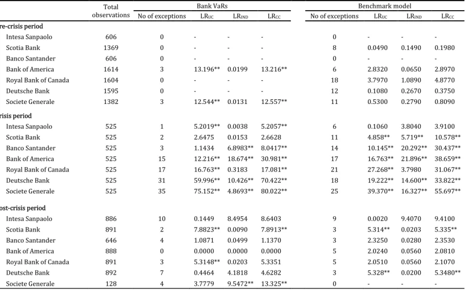
Table 2.7 Performance evaluation of bank VaRs and the benchmark model ... 64

Chapter 3

Table 3.2 Unit root test of daily P/L of sample banks ... 87

Table 3.3 Parameter estimation of GARCH-type models ... 88

Table 3.4 The absolute performance of VaR estimates in pre-crisis period ... 92

Table 3.5 The absolute performance of VaR estimates in crisis period ... 94

Table 3.6 The absolute performance of VaR estimates in post-crisis period ... 96

Table 3.7 The ranking of magnitude Loss Function of VaR estimates using 2-year moving window ... 104

Table 3.8 The ranking of magnitude Loss Function of VaR estimates using 1-year moving window ... 105

Table 3.9 Selection of VaR models ... 106

Chapter 4

Table 4.2 Parameter estimation of the conditional volatility models ... 138

Table 4.3 Coefficient estimation of the LQR-RV model ... 138

Table 4.4 Absolute performance of alternative forecasting models ... 140

Table 4.5 Relative performance of the alternative forecasting models ... 145

Table 4.6 Evaluation of combined quantile forecasts ... 147

viii

List of Figures

Chapter 2

Figure 2.1 Example of data collection method ... 35

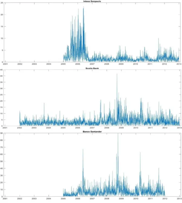
Figure 2.2 Absolute demeaned P/L of commercial banks ... 44

Figure 2.3 Daily trading P/L and VaRs of commercial banks ... 46

Figure 2.4 The three-zone approach ... 54

Figure 2.5 Contribution of trading portfolio to banks’ total assets ... 66

Chapter 3

Chapter 4

ix

List of Abbreviations

CAViaR ... Conditional Autoregressive Value at Risk CC ... Conditional Coverage CQOM ... Conditional quantile optimization method DQ ...Dynamic Quantile EWMA ... Exponentially Weighted Moving Average EVT ... Extreme Value Theory GARCH ... Generalized Autoregressive Conditional Heteroskedasticity GPD ... Generalized Pareto Distribution HAR ... Heterogenous Autoregressive HEAVY ... High Frequency-based Volatility Model HS ... Historical Simulation IND ... Independence LF ... Loss Function LQR ... Linear Quantile Regression LR ... Likelihood Ratio LS ... Logarithmic Score MLE ... Maximum Likelihood Estimation MRA ... Market Risk Amendment MUC ... Multivariate Unconditional Coverage P/L ... Profit and Loss POT ... Peak over Threshold QS ... Quantile Score RV ... Realized Volatility UC ... Unconditional Coverage VaR ... Value at Risk VCV ... Variance - Covariance WQS ... Weighted Quantile Score WTI ... West Texas Intermediate

1

Chapter 1: Introduction

During the 1970s and 1980s, a number of financial institutions built internal models to measure, aggregate and manage exposures across their business lines. However, as the activities of financial institutions became more and more complex, aggregating exposures across business lines become increasingly difficult because of the high correlations amongst risk factors. Financial institutions also lacked the means to managing risk across progressively diverse positions. The absence of integrated risk management demanded tools that measure the probability of loss at institutions-wide level. This led to the development of Value-at-Risk (VaR). VaR is a comprehensive solution to the problem of how to measure the risk taken by an increasingly complicated global bank.

The first VaR model was developed in the early 1990s in the back-office of JP Morgan. Following an order from the CEO to develop a system that measures risk across different trading positions, a single risk measure was developed. Early in 1994, JP Morgan introduced its Riskmetrics service − a simplified version of their internal VaR model. Later that year, JP Morgan published Riskmetrics system, and gave free access to it on the internet. The promotion of Riskmetrics provided a major boost to the ideas surrounding VaR system. Indeed, the adoption of VaR was rapid, amongst security firms, investment and commercial banks and other financial institutions. The VaR concept became increasingly popular, and by the mid-1990s, it was regarded as the dominant measure of market risk (Down, 2005).

VaR aims to capture the market risk of a trading portfolio. VaR is a numerical measure that determines the maximum potential loss on a portfolio within a given

2

time horizon, and using a given level of confidence (Jorion, 2006). The concept is attractive and transparent and is widely regarded as a benchmark for measuring market risk. Beside profitability, a manager only needs to worry about the regulatory boundary measured by VAR, at the tails of their profit and loss (P/L) distribution. At institutional level, VaR has been used for risk management, and in public disclosure and financial reporting, as well as in the computation of regulatory capital requirements. Accurate VaR estimates are crucial for financial institutions as misleading VaR estimates can lead to sub-optimal capital allocation.

VaR is also used as a regulatory tool for ensuring the soundness of the financial systems. In 1996, the Basel Committee on Banking Supervision (BCBS) issued the Market Risk Amendment (MRA) to the first Basel Capital Accord, placing a milestone on the use of VaR. Indeed, the MRA allows financial institutions to use their internal VaR model to measure and disclose market risk. Following the BCBS support for VaR, regulators demanded that all financial institutions estimate and disclose their VaR measures in their financial reports.1 _{The first time VaR was} recognised in financial regulation was in 1997, when the U.S. Securities and Exchange Commission ruled that public corporations must disclose quantitative information about their derivatives trading and derivatives position. Major banks and dealers implemented the ruling by including VaR information in the notes to their financial statements. The Basel II Accord, which came into effect in January

3

20072_{, also strongly promotes VaR estimates as the preferred market risk} management approach.3

VaR has some key drawbacks. Most VaR estimates rely on the normality assumption even if the observations from the empirical distribution is not normal. Risk is a matter of the behaviour in the extreme tails of a distribution. As Greenspan (1997) notes, that the biggest problem with risk management is the measurement of the fat-tailedness of a distribution. In fact, the occurrence of the recent financial crisis has partly been attributed to the failure to acknowledge the role of the fat-tails in VaR estimates (Triana, 2009). The use of VaR has also been blamed for providing little warning of the potential loss for banks during crisis periods (Nocera, 2009). Although details regarding the poor performance of bank VaRs is not new, it is surprising that VaR estimates of banks have received very little attention in empirical work. Therefore, this thesis aims to provide an empirical evaluation on the performance of VaR estimates provided by banks and the factors that affect the reliability of their VaR estimates.

This thesis consists of three empirical essays on the VaR estimates at banks. Chapter 2 contributes to the VaR literature by investigating the performance of bank VaRs for a set of international banks. Our dataset includes the daily trading P/L and VaR of seven commercial banks from January 2001 to December 2012, covering the

2 _{Basel II came into effect in the European Union on 1 January 2007 under the Capital Requirements}

Directive (CRD) and all lenders covered by the CRD have had to implement it from the beginning of 2008. The US delayed this date to January 2009.

3 _{The Basel II Capital Accord is a set of recommendations on banking regulation that is applicable to}

all banks in order to stimulate the improvement of risk management. Clients’ commitment to Basel II compliance can be demonstrated to regulators through their evidence of systematic VaR backtesting. In the first pillar of Basel II, for market risk the preferred approach is specified as Value at Risk.

4

pre-crisis, financial crisis and post-crisis periods. Using the coverage tests, we find that bank VaRs were conservatively estimated in pre-crisis and post-crisis periods. During financial crisis, while some banks continued to overstate their VaR, the others remarkably understated their risk. We quantify the VaR distortions for seven sample banks and find that the VaR overstatement/understatement levels at large banks are more serious than small banks. We also find evidence of extreme losses during financial crisis which probably exceed the market risk capital requirements of banks. We attribute the poor performance of bank VaRs to three main causes: the use of contaminated data, the choice of VaR model and the benefit of VaR overstatement. The distortions of bank VaRs, which are popular across banks, make VaR a poor risk management tool.

The second empirical study (Chapter 3) investigates the forecasting power of VaR models using dataset of trading P/L of seven banks from January 2001 to December 2012. We compare the performance of internal VaR model at banks to alternative VaR approaches, including the Historical simulation (HS), the Variance-Covariance (VCV) and the Extreme Value Theory (EVT) approaches. To compare model performance, we develop a two-stage backtesting that examines the absolute and comparative performance of VaR models. The empirical analysis shows two main points. First, we find that the alternative VaR models can easily outperform banks’ internal model in both normal and crisis periods. Second, we document the superiority of the GARCH-type models in providing good VaR estimates at banks. While the HS models perform inconsistently, none of the banks’ internal model accurately capture the bank risk. The EVT approach, which was shown to be superior in VaR estimation with market data, performs very poorly with bank data.

5

Thus, we argue that good bank VaRs can be obtained using simple and accessible models rather than other sophisticated models or internal VaR model at banks.

The third empirical study (Chapter 4) explores VaR estimates with high-frequency data. This chapter provides the first assessment of quantile combinations, using high-frequency data. In this study, we use the 5-minute sampling data of WTI Crude Oil Futures as oil market is important for desk level trading at banks. The findings of this study are twofold. First, we acknowledge the value of the high-frequency data on the measure of volatility to characterize the quantile forecast of asset returns. Second, we find that the use of quantile combination can improve the accuracy of quantile forecasts. To find whether the use of high-frequency data can improve quantile forecast accuracy, we compare the performance of the GARCH(1,1) models to the Realized Volatility (RV) - based models, including the Heterogenous Autoregressive model (HAR-RV) of Corsi (2009), the High-frEquency-bAsed VolatilitY (HEAVY) model of Shephard and Sheppard (2010) and the RV-based Linear quantile regression (LQR-RV) of Zikes and Barunik (2016). Evaluating their absolute and comparative performance, we find that the HEAVY and HAR-RV model outperform the GARCH(1,1) models across quantile levels and forecast horizons. To to examine the power of quantile combination in improving forecast accuracy, this chapter uses the Conditional quantile optimization method (CQOM) of Halbleib and Pohlmeier (2012) to combine individual quantile forecasts. We find that the combined forecasts are superior stand-alone forecasts in providing accurate and robust results, not only at 1%-quantile (VaR), but also across all quantile thresholds and forecast horizons.

6

The thesis proceeds with three empirical studies in Chapter 2, Chapter 3 and Chapter 4, while Chapter 5 summarizes the findings of the thesis.

7

Chapter 2: Value-at-Risk models

and commercial banks

2.1 Introduction

In the financial industry, Value-at-Risk (VaR) has become a standard risk measurement technique in finance. VaR specifically aims to capture the market risk of portfolios (Jorion, 2006), which is regarded as the maximum potential loss for a given period, normally one-day-ahead, using a certain level of confidence, typically the 95% or 99%. The VaR idea provided a comprehensive solution to identify an acceptable level of risk for an increasingly complicated global bank. In 1992, JP Morgan introduced its Riskmetrics service, in which it published the methodology and gave free access to the estimates of the necessary underlying parameter. Since then, the use of VaR has been promoted widely. However, only when the Basel Committee put forward the Market Risk Amendment (MRA) to the Capital Accord in 1996 made VaR become a benchmark for measuring market risk. VaR became a part of regulatory banking in 1997, when the U.S. Securities and Exchange Commission ruled that public corporations must disclose quantitative information about their derivatives trading activity. Major banks and dealers chose to implement the rule by disclosing VaR information on their financial statements.

The requirement of VaR disclosure has some main objectives. Firstly, it presents an aggregated estimate of the market risk value under taken by a bank. VaR also presents asymmetric information about the bank to market participants and investors. Secondly, result of VaR estimates can be converted into a capital charge to provide an adequate cushion for cumulative losses caused by adverse

8

market conditions. More importantly, the disclosure of VaR estimates allows financial regulators to examine the validity of bank’s internal VaR models. An assessment of these internal VaR models is provided in this thesis, using a procedure called “backtesting”.

Backtesting is a technique which aims to investigate the forecasting power of a VaR model by periodically comparing the VaR estimates generated by the model with the actual P/L (or “trading outcome”).4 _{Our test is performed using daily data.} Backtesting therefore identifies situations where VaR is underestimated (or a VaR exception), meaning that the portfolio has experienced a loss greater than the estimated VaR. The comparison between the risk measures with trading outcome, simply means that the financial institution counts the number of VaR exceptions. That is, the number of occasions that losses exceed the estimated VaR. The frequency of VaR exceptions is then compared with the intended level of coverage to assess the performance of the risk model.

An estimate of the number of VaR exception is asymmetric in nature. Recall that a VaR exception occurs only when the risk is underestimated. Therefore, simply over-estimating VaR can reduce the number of VaR exceptions. This creates an incentive to overstate VaR. Indeed, the current Basel backtesting framework relies on the number of VaR exception to evaluate the performance of internal VaR models.5 _{Specifically, banks are penalized if their VaR model produces too many}

4 _{BCBS, 1996b}

6 _{A trading book consists of positions in financial instruments and commodities held either with}

trading intent or in order to hedge other elements of the trading book. To be eligible for trading book capital treatment, financial instruments must either be free of any restrictive covenants on their tradability or able to be hedged completely. In addition, positions should be frequently and accurately valued, and the portfolio should be actively managed (Basel Committee on Banking Supervision, 2004)

9

exceptions. However, there is no capital charge for banks that have no VaR exceptions. Therefore, even using the Basel backtesing framework incentivizes banks to overstate their VaR estimates.

Investigating the accuracy of bank VaRs is an important area of academic research. It is obvious that VaR models are only useful when they accurately forecast risk. If not, an inaccurate VaR estimate can cause financial institutions to underestimate (or overestimate) their risk, thereby providing misleading indicators of risk. The performance of VaR models also has direct impacts on the calculation of the market capital risk. According to the MRA, the accuracy of VaR models results in the use of a multiplier to convert VaR estimates into the minimum capital requirement for market risk. Banking regulators only allow a bank’s internal VaR model to be used for regulatory capital computation, if the model provides satisfactory backtesting results. Specifically, a VaR model that fails a backtest will be reviewed and will either be disallowed in computing regulatory capital, or be subject to high capital multiplier.

In the literature, bank VaRs perform variously. As Lucas (2001) notes, banks have incentives to under-report VaR estimates to lower their cost of capital, although this can lead to an increase in the probability of VaR exceptions. On the other hand, there are evidences showing that banks excessively overstate their VaR estimates (see Berkowitz and O’Brien, 2002; Perignon et al., 2008; Perignon and Smith, 2010; O’Brien and Szerszen, 2014) as they want to minimise the likelihood of having many VaR exceptions to avoid reputational costs. Bank VaRs are also controversial since they cannot outperform VaR forecasts produced by simple

10

econometric models, such as GARCH(1,1) (Berkowitz and O’Brien, 2002; Perignon et al., 2008; O’Brien and Szerszen, 2014).

The recent global crisis raised a number of questions regarding to the reliability of VaR estimates at financial institutions. Indeed, VaR was blamed for the financial crisis, as it dangerously produces too low risk figures by borrowing the past data and using the improper probabilistic assumptions (Triana, 2009). Although the poor performance of bank VaRs is not new, there has been little empirical study on this topic, due to the proprietary nature of the P/L and VaR data. Indeed, the performance of bank VaRs in crisis period has only been examined by O’Brien and Szerszen (2014) with the empirical evidence of US banks. To the best of our knowledge, there has been no empirical study on the accuracy of bank VaRs on international level. Besides, the performance of bank VaRs in post-crisis period still has not been covered in the literature.

Chapter 2 contributes to the literature as the first investigation on the performance of bank VaRs covering the pre-crisis, financial crisis and post-crisis periods. Our dataset includes the daily P/L and VaR of seven commercial banks from 2001 to 2012. Instead of focusing on a specific country, this chapter investigates bank VaRs on international level. Our dataset includes Scotia Bank, Royal Bank of Canada (Canada), Banca Intesa (Italy), Banco Santander (Spain), Societe Generale (France), Deutsche Bank (Germany) and Bank of America (USA). Compared to prior studies, we use longer and more diversified dataset. The rich dataset not only increases the power of the statistical tests, but also allows us to have a comprehensive evaluation of bank VaRs in international perspective. Besides, this

11

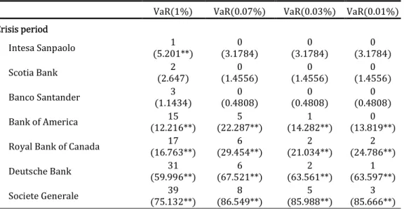
study employs the innovative Multivariate Unconditional Coverage (MUC) test of Colletaz et al. (2013) to examine the presence of extreme losses that exceed VaR at very low coverage rates e.g. VaR(0.07%), VaR (0.03%) or even VaR(0.01%). To the best of our knowledge, the investigation of extreme losses during financial crisis has not been studied in the literature.

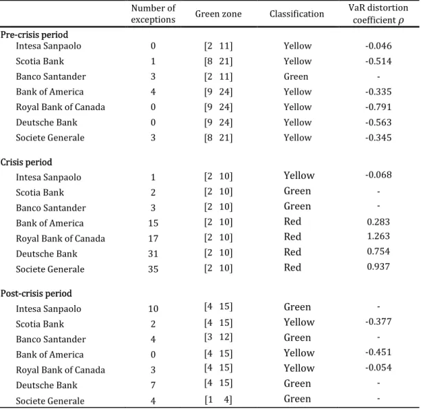
Our empirical analysis shows the poor performance of bank VaRs. We find that bank VaRs tend to be conservatively estimated in normal periods. During financial crisis, while some banks continue to overstate their VaR, the others significantly underestimate their risk. In case of VaR understatement, the number of VaR exceptions are excessively high and tend to cluster together. We find evidence of extreme losses during financial crisis that can exceed VaR at very low coverage rates e.g. VaR(0.07%), VaR(0.03%) or even VaR(0.01%). We attribute the poor performance of bank VaRs to the use of contaminated data, the choice of VaR model and the benefit of VaR overstatement. Due to the fact that the performance of bank VaRs does not improve overtime, we argue that banks accept their inferior VaR models and conservatively estimate their risk to have the economic merit of VaR overstatement. The manipulations of bank VaRs, which are popular across banks, make VaR a poor risk management tool.

Chapter 2 is presented as follows: Section 2.2 introduces background of VaR and their backtesting. Section 2.3 reports the preliminary analysis of sample banks and their daily trading P/L. Section 2.4 presents the empirical investigation of bank VaRs. Section 2.5 discusses the potential causes of the poor performance of bank VaRs, while Section 2.6 summarizes the main results of the chapter.

12

2.2 Value-at-risk and Backtesting Value-at-risk

2.2.1 Value-at-risk background

From an economic point of view, risk is uncertainty about future outcomes. Risk is a key element in the financial world, since firms usually make investment decision under uncertainty as they do not know whether predicted cash flows will materialize. From the 1970s, risk management has become one of the most important tasks of financial institutions since market volatility has increased remarkably after the collapse of Bretton Woods system. Besides, the unexpected catastrophes in 1990s, such as the demise of Barings Bank, Orange County, Long Term Capital Management after significant changes in market conditions, highlighted the demand of effective market risk management. The severity of the recent global financial crisis has also raised the importance of risk management.

The idea of VaR was originated in the late 1970s, when a number of financial institutions developed their internal models to measure and aggregate risk across business lines as a whole. As institutions were becoming more global and complex, with the development of financial products, the aggregation of risks became more demanding when taking into account of how they correlate with each other. During the late 1980s, JP Morgan set up their firm-wide risk management system based on portfolio theory that could model several hundred risk factors and aggregate them into a single financial risk measure. Their measure named Value-at-Risk, the maximum value that can be lost over the next trading day, placed a milestone on the development of market risk measurement. In 1992, at a time of global concerns about leverage and derivatives, JP Morgan introduced their Riskmetrics service to

13

the public, comprising a detailed technical document and a covariance matrix for several hundred key factors, which was updated daily. With the launch of Riskmetrics, VaR was publicized and has been promoted widely.

VaR was originally developed to measure the maximum expected loss caused by movements in the volatility of asset prices for a given portfolio of financial assets. As Linsmeier and Pearson (1996) note, VaR presents as the loss which is expected to be surpassed with the given percent of probability during the next t-day periods. According to Alexander (2009), VaR is the potential loss that will not be exceeded if the given portfolio is held over some periods of time. With a given significant level α and set p = 1- α as level of confidence, and denote qα as the α -quantile of the P/L of a portfolio over a holding period ht, then the VaRα,ht of the portfolio is defined as: VaRα,ht = qα (2.1)

The magnitude of VaR depends on two fundamental parameters: the significant level α (or 1- α level of confidence) and the holding horizon ht. For instance, suppose a bank discloses their VaR on trading portfolio is $50 million with 99% level of confidence and the forecast horizon is one-day-ahead. It means that over the next working day, there is a 99% probability that if the bank suffers a loss, its magnitude will not exceed $50 million. In other words, there is only 1% probability that over the next working day, the loss will be greater than $50 million.

The significance level α is usually set by an external body (banking regulator, credit agency). Under the Basel Accord, banks are required to use 1% significant level (or 99% level of confidence) to determine their market risk capital requirement. Besides, credit rating agencies may be stricter in setting their

14

significance level, which means a higher confidence level (e.g. 99.7% or 99.9%). In the absence of a regulated financial environment and external agencies, the confidence level for the VaR model can depend on the attitude to risk of managers. The more conservative the risk manager, the lower the value of α, i.e. the higher the level of confidence applied (Alexander, 2009). Dowd (1998) indicates that if investors want to validate a VaR model, the high level of confidence (such as 99% or 99.5%) should be avoided to be able to observe enough VaR exceptions. On the other hand, the risk appetite of senior management plays a significant role in selecting the level of confidence. Besides, the choice of risk horizon ht also depends on the nature of each asset’s volatility and degree of liquidity. For the investors who actively make money via trading in equity market, typically the 1-day risk horizon is appropriate, whereas institutional users and non-financial institutions may prefer longer risk horizon (Linsmeier and Pearson, 1996).

One of the main attractions of VaR is that it is presented in a simplest way with most understood unit of measure. By simplifying the assumptions used in its computation, VaR aggregates the diversification effects, leverage effects and probabilities of adverse price movements to single dollar value that is suitable for application and communication with interested parties. Besides, VaR has number of attractions over traditional risk measures. Firstly, VaR can be universally applied to any types of portfolio. It allows us to compare the risks between two different portfolios. Secondly, VaR enables us to aggregate the risk of desk-level portfolios into an overall measure of portfolio risk while taking into account the way different risk factors interact with each other. This characteristic is especially important, as financial institutions are exposed to a variety of market risks. Besides, VaR is

15

probabilistic, which provides risk managers helpful information on the probability associated with specified loss. Thus, VaR is regarded as the most important quantitative risk measure used by financial institutions (Woods et al., 2008).

VaR also has limitations. The main drawback is that as a measure of market risk, it tells you nothing about the potential loss that would break the VaR threshold when extreme event occurs. A VaR figure at 99% level of confidence has no information about how much the unexpected loss might be in the 1% tail of the P/L distribution. The omission of VaR in order to take into account the magnitude of exceeded loss makes it unable to differentiate between two positions being given the same VaR figure but have very different risk exposures. Besides, the dependency on the normality assumption is other serious limitation of VaR. In normal market condition, VaR works reasonably well. But VaR is not reliable when financial markets are excessively volatile and during financial crises (Dowd, 2005).

VaR information can be used in various ways. First, senior risk managers can use VaR to set their overall risk target, and from that determine risk figures and position limits for each business line. If they want to increase the risk of financial institution, they would increase the overall VaR threshold or, vice versa. Secondly, VaR can be useful to calculate capital requirements, both at the institutional scale and business-unit level with the driving principle: the riskier the trading activity, the higher the VaR figure and the greater the capital requirement. Besides, VaR figures can be used for the purpose of reporting and disclosing financial risk, and financial institutions increasingly make a point of disclosing VaR information in their annual reports (Dowd, 2000; Jorion, 2002; Woods et al., 2008). VaR is also

16

informative not only for making decisions of investment, trading, hedging and portfolio management, but also setting limits on the rule that apply when rewarding managers in order to discourage excessive risk taking (Dowd, 1999; 2005).

2.2.2 Basel Capital Accord and market risk management

The Basel Committee on Banking Supervision (BSBS) was originated during the period of financial market turmoil after the breakdown of the Bretton Woods system in 1973. Aiming to improve financial stability by enhancing supervisory knowhow and the quality of global banking supervision, the Committee sets minimum standard of supervision and regulations of banks, where capital adequacy becomes the main focus. Backed by G10 Governors, the first Basel Capital Accord (Basel I) was published in 1988 to set up a minimum ratio of bank’s capital to risk-weighted assets of 8% and has always been improved overtime to make it adapt to current financial situations. It is worth to emphasize that this framework only covers the credit risk in evaluating capital adequacy. Under this accord, all assets in bank’s balance sheet are given a judgemental risk classification with a fixed risk weight from 0 to 100 percent.

Various amendments were made over years to extend the definition and effects of credit risk (in 1991 and 1995 Amendments), but the most important one was the MRA to the Capital Accord issued in 1996. These evolutions took place after the number of failures in risk management (e.g. Orange County, Procter and Gamble) that raised the concern about financial derivatives and called for effective regulation of financial market. During that period, industry also issued a number of best practice reports of how to manage the risk of financial derivatives, one of those

17

was appeared in G30 report in 1993. This influential report then became the handbook of financial risk management discipline, and its best practice guidelines were globally accepted by both industry and regulators, which were also presented in 1996 Amendment. In particular, the 1996 MRA specified banks’ exposure to interest rate related instruments and equities in the trading book6 _{and commodities} risk and foreign exchange risk throughout the bank. In this Amendment, banks have option to choose either the standardised method or internal model based approach for meeting market risk capital requirements. The first option specifies the measurement of risk for each category from foreign exchange, equities, commodities and derivatives.

In MRA, banks are allowed to use their internal VaR models to measure their market risk, which is subject to strict qualitative and quantitative standards. In internal model approach, banks are flexible in developing their own models, but required to follow minimum standards for the purpose of their capital charge. For some main points, VaR must be calculated on a daily basis with the minimum holding period of 10 trading days7 _{at 99}th _{percentile and one-tailed confidence} interval. A minimum length of one year for historical data is needed to compute VaR, which is also subject to the update and revision requirement no less frequently than once every three months. Banks that use internal model approach are also subject

6 _{A trading book consists of positions in financial instruments and commodities held either with}

trading intent or in order to hedge other elements of the trading book. To be eligible for trading book capital treatment, financial instruments must either be free of any restrictive covenants on their tradability or able to be hedged completely. In addition, positions should be frequently and accurately valued, and the portfolio should be actively managed (Basel Committee on Banking Supervision, 2004)

7_{Banks can use VaR numbers computed regarding to shorter holding periods scaled up to ten days}

18

to use comprehensive stress testing program to identify extreme events that could significantly impact banks. The issue of MRA to the Capital Accord made the popularity of VaR reach to its peak, where VaR model was globally accepted as a benchmark of market risk management and only few people could recognize its weaknesses. With the adoption of MRA, it was the signal that bank regulators accepted and stood on the principle of risk-based regulation.

By second half of 1990s, banking activities were becoming more sophisticated and risk modelling was quickly evolving that called for a major advancement of Basel Accord. In 1999, the new capital adequacy framework was proposed to better capture bank’s risk taking and reflect the financial innovation. The Revised Capital Framework, generally known as Basel II, was officially released in 2004. Basel 2 consists of three pillars: (i) The first pillar: minimum capital requirements, which sought to develop and expand the standardised rules set out in the 1988 Capital Accord; (ii) The second pillar: supervisory review of capital adequacy and internal assessment process; and (iii) The third pillar: effective use of disclosure to enhance market discipline and encourage sound banking practices.

Basel II made a major enhancement in credit risk modelling and for the first time, covered the operational risk within the first pillar of the accord, but for market risk measurement there was no noticeable changes from Basel I to Basel II. In Basel II, the market risk disclosure requirement was clearly presented in the third pillar in both qualitative and quantitative aspects. For banks using standardised approach, the disclosure of capital requirements for all sources of risk (e.g. interest rate risk, equity position risk, foreign exchange risk and commodity risk) is needed.

19

Banks using internal model approach are required to disclose their qualitative information about the features of models employed, the description of portfolio’s stress testing and the characteristics of backtesting process. In term of quantitative disclosure, they are required to present VaR values (e.g. high, mean and low VaR) over the reporting period and period-end, coming with the comparison of VaR estimates with actual P/L and the analysis of remarkable VaR exceptions.

According to the Basel capital accord, VaR estimates are based on one of two theoretical assumptions about a trading portfolio. First, the trading portfolio is assumed to be rebalanced over the risk horizon to keep the risk factor sensitivities or asset weights constant. Second, the trading portfolio is assumed to be held static such that no trading occurs during the period. However, both assumptions are unrealistic. In practice, trading portfolios are actively managed, and the actual P/L on the trading portfolio is not equal to the hypothetical P/L, on which VaR estimates are based. Indeed, the hypothetical P/L is the mark-to-market P/L, while the actual P/L includes all the P/L amounts from intraday trading, fees and commissions (using actual prices). Therefore, it is important to regularly revise VaR models and their performance using backtesting.

2.2.3 Value-at-Risk at commercial banks

VaR has become the standard market risk measurement at commercial banks since the publication of the MRA. Allowed to use internal models to estimate VaR, banks can be flexible in improving their existing models although they are required to follow minimum standard.

20

The MRA has no legal force. Instead, it formulates supervisory guidelines and standards. Corresponding to the international guidelines, domestic financial regulators require commercial banks to compute and publicly disclose their VaRs in annual reports. For example, the US commercial banks are required to publicly disclose their market risk under Financial Reporting Release Number 48, issued by SEC in 1997. In Canada, the Office of the Superintendent of Financial Institutions has required financial institutions to compute and publicly disclose their VaR since the late 1990s. The disclosure of VaR has some main targets. First, VaR provides a universal measure of amount of market risks suffered by a bank, aiming to reduce the asymmetric information between the bank and the public. Second, VaR can be translated into capital charge, which is supposed to be a cushion for cumulative losses. In addition, VaR disclosure allows financial regulator to evaluate the performance of bank’s internal VaR model through the process of “backtesting”.

2.2.4 Backtesting Value-at-Risk

It is obvious that VaR model is only useful when it forecasts risk reasonably well. If not, it can lead financial institutions to underestimate (or overestimate) their risk and hence provide misleading managerial guidelines. Therefore, after constructing VaR model, it is important to regularly evaluate the adequacy of the VaR model used.

Backtesting is a technique which aims to investigate the forecasting power of the VaR model by comparing the risk estimates generated by the model against actual daily changes in portfolio value over longer periods of time. Backtesting therefore identifies situations where VaR has been underestimated, meaning a

21

portfolio has experienced a loss greater than the original estimated VaR. The comparison between the risk measures with trading outcome simply means that the financial institution counts the number of VaR exceptions, a situation when a loss is greater than the estimated VaR. The frequency of VaR exceptions is then compared with the intended level of coverage to assess the performance of the risk model. The results of the backtesting can be informative to refine the model used for the VaR predictions, making them more accurate and reducing the risk of unexpected losses. The backtesting framework recommended by Basel committee includes the use of one-day-ahead VaR estimates and one-day trading outcomes, excluding any intra-day revenues, fees and commissions. It is straightforward to implement the Basel backtest, simply by computing the frequency of VaR exceptions – the cases that the trading P/L are not covered by the VaR estimates. With approximately 250 trading days in a fiscal year and 99% level of confidence, banks are expected to have about three VaR exceptions per year. Depending on the actual number of VaR exceptions, the backtest result can be classified into one of three zones. That is Green zone (0 to 4 exceptions), Yellow (5 to 9 exceptions) or Red (10 exceptions or above). Different zones are subject to different level of capital charge. Thus, the more VaR exceptions, the higher the charge.

The three-zone backtesting approach of Basel committee has some drawbacks. First, it is specified for evaluating VaR models for one year, with approximately 250 observations. Second, it primarily assumes that each day’s test outcome is independent from each other’. This assumption is not realistic, due to the fact that VaR exceptions tend to cluster together, especially during crisis period.

22

Besides, the Basel framework does not penalize banks that overstate their VaRs to maintain low number of VaR exceptions. From risk management perspective, the estimated return at the lower tail defines the amount of capital that banks allocate to cover the possible loss, which is called the economic capital for market risk. The low number of VaR exceptions means that the tail is overestimated and therefore signals an excessive amount of allocated capital.

To overcome these shortcomings but still preserve the frequency-based approach of Basel framework, this chapter uses several coverage tests to evaluate the performance of bank VaRs, including: (i) the Unconditional Coverage (UC) test of Kupiec (1995); (ii) the Conditional Coverage (CC) test of Christoffersen (1998); and (iii) the Multivariate Unconditional Coverage (MUC) test of Colletaz et al. (2013). Each test has different power. The widely-used UC test aims to quantify and investigate the frequency of VaR exceptions, while the CC test additionally examines the assumption of independence of VaR exceptions. Besides, the MUC test allows us to jointly examine the coverage and comparative magnitude of extreme losses. 2.2.4.1 The Unconditional Coverage test

As the name suggests, the UC test examines the coverage of VaR exceptions based on the actual number of VaR exceptions. It is worth noting that the frequency of VaR exceptions plays a crucial role in validating the adequacy of VaR estimates. The Group of Thirty (G30) recommends that financial institutions carry out reality checks to evaluate the performance of their VaR models.8 _{Specifically, it is} recommended that an institution’s VaR estimates are compared against actual

23

portfolio outcomes. In line with the G30’s idea, the Basel Committee proposes a “traffic light” backtesting framework, which relies on the number of VaR exceptions, to verify the accuracy of internal VaR models.9

Let rt denote P/L of a given portfolio at time t and VaRt|t-1(α) the one-day ahead VaR forecast for a given α coverage rate conditional on an information set Ωt-1. If the VaR estimates are adequate, the UC property states that:

Pr [rt< VaR t|t-1(α)] = α (2.2)

Let It(α) be a hit indicator variable associated with the VaR exception at time t, in which:

It(α) = V 1 if rW< VaRW|WXY(α)

0 otherwise (2.3)

The null hypothesis of UC property is that the observed frequency of VaR exceptions is consistent with the nominal frequency α, thus:

H0: E [It(α)] = α and H1: E [It(α)] ≠ α (2.4) To satisfy the UC property, the likelihood of which actual P/L on day t exceeds its corresponding VaRt|t-1(α) must be equal to α x 100%, or Pr [It(α) =1] = α. The null hypothesis is rejected if the difference between observed frequency of VaR exceptions and the expected rate α, is statistically significant. Therefore, there are two occasions when UC hypothesis can be rejected. The first is the case of overestimation, when the realized frequency of VaR exceptions is smaller than the nominal rate α, or Pr [It(α) = 1] < α. The second is when the VaR underestimation

24

occurs and the realized frequency of VaR exceptions is higher than the nominal rate α, or Pr [It(α) = 1] > α.

Let T0 and T1 be the number of zeros and ones corresponding to the hit indicator variable (2.3). Let T be the total number of observations, thus T = T0 + T1. The Log-likelihood ratio statistics of the UC hypothesis, denoted as LRUC, is given by: LRUC(α) = - 2ln[(1 − α)]^ α]_] + 2ln`(1 − ]_]_)]^ (]_]_)]_a → χd(1) (2.5) The LRUC converges to an asymptotically Chi-square distribution with one degree of freedom. Recall that UC text examines whether the empirical frequency of VaR exceptions N/T is sufficiently close to the predicted α. The null hypothesis H0 is not rejected if the empirical frequency of VaR exceptions is close enough to the coverage rate α. There are some examples of non-rejection regions for the UC test. If the sample size T = 250 (one year), for a 5% nominal size the UC assumption is not rejected if the total number of VaR(1%) violations is strictly from 1 to 6. In case T = 500, the total number of exceptions must range from 1 to 11 in order to satisfy the UC hypothesis.

2.2.4.2 The Conditional Coverage test

The CC test extends the UC test by jointly examining the IND and UC properties of VaR exceptions. As Christoffersen (1998) notes, the IND hypothesis holds when VaR exceptions occurring at two different times for the same coverage rate are independently distributed. In other words, the hit indicator {It(α) =1} corresponding to VaR exception at time t, at coverage rate α, is independent from hit process {It-k(α) =1}associated with the VaR exception at time t-k, ∀k ≠ 0. This

25

assumes that past exceptions do not hold information on current and future VaR exceptions. Thus, the rejection of the IND hypothesis may imply a clustering of VaR exceptions.

The LR test statistic for IND hypothesis is given by:

LRIND = -2ln[(1 - ]_]_)]^ (]_]_)]_ ] + 2ln[(1 - πh01)]^^πh_iY]^_ → χd(1) (2.6) where Ti,j, i, j =0, 1 is the number of observations with a j following a i in the hit indicator variable It, and πh01=_] ]^_

^^j]^_. The LRIND follows Chi-square distribution

with one degree of freedom.

The CC test simultaneously examines the UC and CC hypotheses. The test statistic for CC hypothesis is presented as:

LRCC = LRUC + LRIND → χd(2) (2.7) The LRCC test statistic converges to the Chi-square distribution with two degrees of freedom. The null hypothesis of CC holds when VaR model satisfies both UC and IND hypotheses. Therefore, the rejection of the CC hypothesis may come from the rejection of the UC and/or IND tests. The CC test allows us to test each hypothesis separately to see whether the model provides incorrect coverage or causes violation clustering.

Although being widely applied by both academia and practitioners, the CC has the key drawback, as it does not account for the magnitude of excessive losses. Specifically, the CC test cannot identify and evaluate the presence of extreme loss, which is far beyond normal VaR. This drawback can be overcome with the use of MUC test.

26

2.2.4.3 The Multivariate Unconditional Coverage test

The MUC test was proposed by Colletaz et al. (2013). The innovation of the MUC is that it gives another view to the performance of a risk model by jointly examining the number and magnitude of extreme losses, in case that an actual loss might not only violate the normal VaR defined with a coverage rate α (i.e. 1%), but also exceed VaR at lower probability α’ (i.e. 0.2%).

In this approach, a VaR exception is the state when rt< VaRt(α), while a VaR super exception take places when rt< VaRt(α’), with α’ smaller than α. In other words, a super exception for VaR defines a situation of excessive losses which not only exceed normal VaR(α), but also break VaR at rare coverage rate, VaR(α’). Therefore, if the frequency of super exceptions is remarkably high, this means the magnitude of the losses associated with VaR(α) is too large.

Estimation of VaR(α’)

Firstly, we demean the P/L series by subtracting the unconditional mean µ from each observation to get the new return series ut, with E(ut) = 0. To estimate VaR(α’) of the P/L series, we firstly estimate VaR(α’) of the demeaned series ut. Then, the VaR(α’) of the P/L series is obtained by adding the unconditional mean µ to the VaR(α’) of the demeaned series ut. We present the method to estimate VaR(α’) of the zero-mean return series ut as following.

As E(ut) = 0, the conditional VaR of the demeaned series ut can be presented as a function of the conditional variance of the return series, denoted as ht:

27

where F-1_{(α; β) is the α-quantile of a standardized conditional P/L distribution,} which is assumed to be parametric associated with a set of parameters β.

Colletaz et al. (2013) propose a method to extract VaR(α’) from VaR(α). Given the disclosed bank VaRs, VaR(α), an implied P/L conditional variance is defined as:

phqW = - rst_xv_u|uv__{(w; yz)}(w) (2.9)

With the idea of option pricing, VaR(α’) is now obtained by: VaRt|t-1(α’, βq) = -phq_W FXY(α; βq) = VaRt|t-1(α)x

v__{(w’; yz)}

xv__{(w; yz)} (2.10) To implement this method, we need two ingredients: (i) the auxiliary model for the conditional volatility ht and (ii) the P/L distribution which is conditional on a set of parameters β. We follow Colletaz et al. (2013) to employ GARCH as auxiliary model and Student t distribution for FXY_{(α; βq). Therefore, the set of parameters β,}

which corresponds to the degree of freedom of the Student t distribution, can be obtained by Quasi-Maximum Likelihood estimation. This calibration procedure was shown to provide robust VaR(α’) estimates (Colletaz et al., 2013).

The Log-likelihood ratio test of MUC hypothesis

Colletaz et al. (2013) propose a LR test to examine the MUC hypothesis. Let It (α) be a hit indicator variable corresponding to the VaRt(α):

It(α) = V 1 if rW< −VaRW|WXY (α)

0 otherwise (2.11) and It (α’) denotes a hit indicator variable associated with VaRt(α’):

It(α’) = V 1 if rW< −VaRW|WXY (α′)

28

It is possible to jointly test the MUC null hypothesis of VaR exceptions and VaR super exceptions:

H0: E[It(α)] = α and E[It(α’)] = α’ (2.13) Denote J1,t and J2,t hit indicator variables, and J0,t = 1- J1,t - J2,t = 1 - It(α) where:

J1,t= It(α) - It(α’) = V 1 if −VaRW|WXY (α |_{) < r} W< −VaRW|WXY (α) 0 otherwise (2.14) J2,t= It(α’) = V 1 if rW< −VaRW|WXY (α′) 0 otherwise (2.15)

Now {J},W}}~id are the Bernoulli random variables that take value of 1 with given

probabilities 1-α, α-α’ and α’ respectively. Let Ni = ∑ J]_{W~Y },W} be the count variable corresponding to each Ji,t variable. The Log-likelihood ratio test statistics for MUC null hypothesis (LRMUC) is given by:

LRMUC(α, α’) = - 2ln[(1- α)N0 (α- α’)N1(α’)N2] + 2ln`( €^ ])€^ ( €_ ])€_( €• ])€•a ‚ → χd_{(2) (2.16)}

where T is the total number of VaR estimates. The LRMUC statistic converges to Chi-square distribution with two degrees of freedom.

2.3 Literature on the performance of bank VaRs

Berkowitz and O’Brien (2002) provide the first evidence on the performance of VaR models at banks. Using private daily data of P/L and VaR of six large banking institutions from January 1998 to March 2000, they show that bank VaRs at the 99th percentile are conservative and in some cases, are extremely inaccurate. In particular, the average exception rate is less than a half of one percent across banks,

29

and in some cases VaR estimates were considerably removed from the lower bound of the P/L. Berkowitz and O’Brien (2002) attribute the cause of VaR overstatement to the method of aggregating VaRs across the entire trading portfolio. Indeed, of the banks whose VaRs are more conservative, the global VaR is simply the summation of sub-VaRs across sources of risk. Besides, the regulatory need of higher capital requirement when banks fail the backtest may motivate banks to overstate their VaR. When comparing with the performance of the ARMA and GARCH as the benchmark models, the banks’ VaR forecasts are not better because they could not adequately capture the changes in the volatility of P/L. In brief, Berkowitz and O’Brien (2002) argue that the reported VaR figures are not useful as measures of the actual risk of bank’s portfolio.

Perignon et al. (2008) confirm the continuous conservativeness in VaR estimates of commercial banks. With the use of non-anonymous daily data of the six largest Canadian banks, they provide evidence of systematic VaR overstatement. Some banks experienced one exceedance, while others even had no VaR exceptions during the 6-year period, from 1999 to 2005. This result contrasts to the common wisdom that banks intend to understate their VaR to lower the market risk capital requirement (Cuoco and Liu, 2006). The VaR conservativeness at Canadian banks is consistent with US evidence reported by Berkowitz and O’Brien (2002). Besides, when compared with the simple HS and GARCH(1,1) models, bank VaR models are not superior in producing accurate risk forecasts. Thus, the internal models used by commercial banks do not provide VaR estimates that are reliable to determine capital charges.

30

Instead of using time series of daily P/L and bank VaRs, Perignon and Smith (2010) collect the number of VaR exceptions disclosed on banks’ annual reports to evaluate the performance of bank VaRs. Using the dataset from 66 commercial banks, they confirm the systematic VaR overstatement at banks. Specifically, during the period of 1996-2005, US largest banks experienced only 10 actual exceptions in comparison to an expected exception of 68. In 2005, Canadian banks even overstated their VaR figures more seriously: only 1 exception over the expectation of 13, while in case of international banks, it is 3 over 53 respectively.

O’Brien and Szerszen (2014) investigate the specifications and performance of the VaR estimates of five anonymous US banks before and during financial crisis. The dataset used in their study include daily P/L and bank VaRs reported to the Federal Reserve Board. Their bank data are standardized to keep the anonymity, hence some valuable information about the absolute magnitude of daily P/L and VaR are absent. Consistent with the prior studies, O’Brien and Szerszen (2014) show that bank VaRs were excessively conservative before financial crisis (with very few VaR exceptions). For the 2007-2008 period, bank VaRs were substantially underestimated and exhibited exception clustering. Besides, it is evident that standard GARCH and HS models can produce more accurate VaR estimates compared to those provided by the banks.

It can be summarized that bank VaRs were conservative before financial crisis, but substantially underestimated during crisis period. Besides, prior studies mostly focus on the evaluation of bank VaRs in tranquil period, the condition that VaR normally works well. However, the recent financial crisis witnessed the failure of

31

VaR on unimaginable scale. Given that VaR has been widely criticised, it is surprising that the literature on the performance of bank VaRs during the financial crisis has only been investigated O’Brien and Szerszen (2014). This study provides empirical evidence for US banks. No study has examined the performance of bank VaR models during the post-crisis period. To fill the gap in the literature, this chapter aims to investigate the performance of bank VaRs for a set of banks across six countries. The analysis covers both crisis and post-crisis periods. Given that bank VaRs were intentionally and systematically overstated in the pre-crisis period, we do not expect that banks change their behaviour during and post-crisis period. The following sections investigate the performance of bank VaRs and present the results.

2.4 Empirical analysis

2.4.1 Data collection method and methodology

It is important to note that the daily VaR and P/L data we are concerned with is from the trading book of the bank. Positions of commercial banks can be categorized into two books, which all exposed to market risk: the banking book, including on-balance sheet and off-balance sheet activities, and the trading book, covering positions of instruments in traded market. However, trading book is exposed to market risk in a more transparent way, as its instruments will hold some direct exposure to market risk (Woods et al., 2008). As the VaR figures disclosed by commercial banks are the risk measure of their trading activities, thus we particularly focus on the market risk exposures of the trading book of a bank.

32

To perform the evaluation of bank VaRs, we require time series data of daily VaR and P/L of banks. However, the P/L and VaR data are one of the most confidential data of banks, which only report to top managers and financial regulators. We find that the sources of assessible VaR information are bank’s annual reports and filings. Therefore, to obtain time series data from these sources, we decide to use the data extraction method, which allows us to convert the graph in banks’ annual reports into time series data. Our data collection strategy is inspired by Perignon et al. (2008).

Initially we seek for these largest banks in North America and Europe countries. For each bank, we then look up whether they present a graph of daily VaR and trading revenues in their annual reports. We end up with a sample of banks that disclose VaR backtesting graph in their public documents. This includes seven commercial banks of six major countries: Royal Bank of Canada, Scotia Bank (Canada) Societe Generale (France), Bank of America (USA), Deutsche Bank (Germany), Intesa Sanpaolo (Italy) and Banco Santander (Spain). Their backtesting graphs are then put into our Matlab-based data extraction program.

The technique we used to collect daily VaR and P/L from banks’ public data sources is simply the “Click and Collect” strategy. Firstly, the backtesting graphs are converted using Matlab to define the images as objects. The images are then re-sharpened and re-scaled to make them visibly clear. Adding the vertical lines to the image, we then zoom in, look up and precisely click on each data point. After one “click”, we collect the two-dimensional Matlab coordinates of a data point, which are then converted into graph coordinates. Repeating this procedure, we obtain

time-33

series of daily P/L and bank VaRs. In order to check the robustness of the data collection method, we plot the extracted data in Microsoft Excel and superimpose this graph with the original graph obtained from bank’s annual report. If two graphs match perfectly, this means that our extracted data are accurate. Any mismatches between the two graphs can be fixed by manually adjusting the extracted data until a complete match is achieved.

We present the graphic example of our data collection method in Figure 2.1. The first is the original backtesting graph we collected from 2012 annual report of Scotia bank, including the series of daily P/L (red line) and daily VaR (yellow line), correspondingly. Using the Matlab-based data extraction program, the time-series of daily P/L and bank VaRs are generated from the upper graph. We then put the extracted data into Excel and plot the graph to compare with the former.

The data extraction program helps us collect the dataset of seven commercial banks, starting from 2001 to 2012. However, we cannot get the full dataset of several banks due to the lack of the backtesting graphs in banks’ annual reports in some periods. This includes Intesa Sanpaolo 2004), Banco Santander (2001-2004), Scotia bank (2001) and Societe Generale (2001, 2010-2012). The sample is then divided into three sub-periods: pre-crisis, crisis and post-crisis periods. The pre-crisis period is from the start of the period to May 2007, while the global financial crisis period is from June 2007 to June 2009. The end of the financial crisis period is determined using the National Bureau of Economic Research indicator as the start of the economic recovery10_{. The post-crisis period is after July 2009.}

34

Prior studies focus on VaR performance of banks in a single country. Our study uses the largest data set to date and covers six developed countries. However, there might be potential sources of bias in our data sample. First, market movements in major countries tend to be highly correlated. Second, the choice of banks may not be representatives of the behaviour of all the banks in a specific country. To resolve this bias, future studies should use a larger set of banks across developed and developing countries.

It is also noteworthy that the disclosed bank VaR estimates are available in aggregate form from their financial reports. Constituents of the VaR estimates include interest rate, equity, foreign exchange, commodities and credit spread VaR. Although the nature of trading portfolio varies across banks, we find that interest rate changes is a major source of risk in VaR estimates, followed by equity, credit spread, commodities and foreign exchange rate changes. Commodities and foreign exchange VaR estimates become increasingly important to the aggregated bank VaR amount, especially during and after the financial crisis. Future studies should examine more closely the constituents of bank VaR estimates and simulate the trading portfolio, using market data.

35

Figure 2.1: Example of data collection method

Notes: Figure 2.1 presents an example of our data collection method. The upper graph presents the daily VaR and P/L of Scotia bank in 2012, which was collected from bank’s annual report. The time-series data of P/L and VaRs are generated from the original graph via our graphical data extraction program. To check the robustness of the extracted data, we superimpose the graphic presentation of time-series data, displayed in lower graph, to the original graph. If two graphs are perfectly matched, the extracted time-series data are robust.

Graphic presentation of trading P/L and VaRs in 2012 annual report of Scotia bank

Graphic presentation of extracted trading P/L and daily VaR of Scotia bank

2.4.2 Preliminary analysis of bank trading P/L

2.4.2.1 Descriptive statistics of sample banks

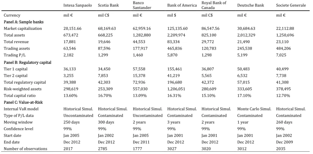
We present the descriptive statistics of seven commercial banks in Table 2.1. Most of figures are collected from banks’ annual reports, except the data of banks’

-30 -20 -10 0 10 20 30 VaR P/L

36

market capitalization are collected from Datastream. In Table 2.1, Panel A reports bank’s market capitalization, total assets, total revenue, trading assets and P/L on trading portfolio. Panel B presents Tier 1, Tier 2 and Total regulatory capital (equal to Tier 1 plus Tier 1 minus adjustme