Washington University in St. Louis
Washington University Open Scholarship
Engineering and Applied Science Theses &
Dissertations McKelvey School of Engineering
Spring 5-2016
Lesion identification and the effect of lesion on
motor mapping after stroke
Ruixi Zhou
Washington University in St. Louis
Follow this and additional works at:https://openscholarship.wustl.edu/eng_etds
Part of theBioimaging and Biomedical Optics Commons,Nervous System Diseases Commons, and theSystems Neuroscience Commons
This Thesis is brought to you for free and open access by the McKelvey School of Engineering at Washington University Open Scholarship. It has been accepted for inclusion in Engineering and Applied Science Theses & Dissertations by an authorized administrator of Washington University Open Scholarship. For more information, please [email protected].
Recommended Citation
Zhou, Ruixi, "Lesion identification and the effect of lesion on motor mapping after stroke" (2016).Engineering and Applied Science Theses & Dissertations. 147.
WASHINGTON UNIVERSITY IN ST. LOUIS School of Engineering and Applied Science
Department of Biomedical Engineering
ThesisExamination Committee: Maurizio Corbetta, Chair
Dennis Barbour
Dan Moran
Lesion identification and the effect of lesion on motor mapping after stroke
by Ruixi Zhou
A thesis presented to the School of Engineering
of Washington University in St. Louis in partial fulfillment of the requirements for the degree of
Master of Science May 2016 Saint Louis, Missouri
ii
Contents
List of Figures ... iii
List of Tables ... iv Acknowledgments ... v Dedication ... vi Abstract ... vii Preface ... ix 1 Automatic segmentation ... 1 1.1 Background ... 1 1.1.1 Existing methods ... 1 1.1.2 Hypothesis ... 2 1.2 Method ... 3 1.2.1 Data acquisition ... 3 1.2.2 Preprocessing ... 4 1.2.3 Unified segmentation ... 5 1.2.4 Abnormalities detection ... 6 1.2.5 Post-processing: clustering ... 7 1.2.6 Interface pipeline ... 9 1.3 Results ... 12 1.4 Discussion ... 15
2 Spatial shift in cortical motor representations post-stroke ... 18
2.1 Background ... 18
2.1.1 Mechanisms of reorganization ... 18
2.1.2 Hypothesis ... 21
2.2 Methods ... 22
2.2.1 Data acquisition ... 23
2.2.2 Surface based registration ... 23
2.2.3 Seed-based approach ... 24
2.2.4 Peak analysis ... 27
2.2.5 Region analysis ... 28
2.3 Results ... 28
2.3.1 Acute stage ... 28
2.3.2 Chronic stage and recovery ... 37
2.4 Discussion ... 43
iii
List of Figures
Figure 1.1: Schematic graph of automatic segmentation ... 3
Figure 1.2: Initial lesion result with default threshold without clustering for subject 105 ... 7
Figure 1.3: Lesion result with threshold = 0.08 and 0.4 without clustering ... 8
Figure 1.4: Main interface for automatic segmentation ... 9
Figure 1.5: Non-clustering and clustering results with threshold = 0.1 for T1 images ... 11
Figure 1.6: Non-clustering and clustering results with threshold = 0.1 for T2 images ... 11-12 Figure 1.7: ROC curve for stroke subject 105 ... 13
Figure 1.8: For all subjects obtain the best lesion results ... 14
Figure 2.1: Seeds covering hand knob on both sides ... 24
Figure 2.2: Atlas generated hand knob seeds overlay on 4 subjects ... 25
Figure 2.3: Left and right hemisphere correlation maps for control subject 003 ... 26
Figure 2.4: Cortical area parcellation based on resting state correlations ... 26
Figure 2.5: Central sulcus mask ... 27
Figure 2.6: Coordinates of peak vertices for healthy subjects and stroke patients ... 29
Figure 2.7: Absolute distances of peaks away from ideal peak ... 31
Figure 2.8: Permutation of variance along three axes ... 32
Figure 2.9: Scatter plots of arm score versus absolute distance ... 33-34 Figure 2.10: Percentage of occurrence for intensity values ... 35
Figure 2.11: Scatter plots of peak intensity versus absolute distance ... 36
Figure 2.12: Average masked correlation maps ... 37-38 Figure 2.13: Mean of x coordinate at two time points ... 39
Figure 2.14: Recovery ratio summary from acute to chronic ... 40
Figure 2.15: Scatter plot of recovery ratio versus absolute shift from acute to chronic on x axis ... 41
iv
List of Tables
v
Acknowledgments
I would like to express my sincere gratitude to my supervisor Dr. Maurizio Corbetta, for providing me the honor to join in his lab. His expertise, patience, understanding and motivation guided me to make this thesis possible.
Except for my advisor, I would like to thank the rest of my committee members: Prof. Dennis Barbour and Prof. Dan Moran, for their insightful comments and great help to my thesis.
I also would like to thank the wonderful people in the Corbetta lab: Prof. Gordon Shulman, Tomer Livne, Joshua S. Siegel, Serguei Astafiev, Hong Xin, Nicholas Metcalf and Dohyun Kim, for their stimulating ideas and generous encouragement.
Special thanks goes to Lenny Ramsey, who has always been mentoring me since my participation in the lab. Without her initial ideas and generous help from the beginning to the end, I cannot finish this thesis.
Ruixi Zhou
Washington University in St. Louis May 2016
vi
Dedicated to my parents, Kai Zhou and Jianping Zeng, for their love and support throughout my life
vii
ABSTRACT OF THE THESIS
Lesion identification and investigation of its effect on motor mapping after stroke
by Ruixi Zhou
Master of Science in Biomedical Engineering Washington University in St. Louis, 2016 Research Advisor: Professor Maurizio Corbetta
Stroke is the most common cause of long-term severe disability and the motor system that is most commonly affected in stroke. One of the mechanisms that underlies recovery of motor deficits is reorganization or remapping of functional representations around the motor cortex. This mechanism has been shown in monkeys, but results in human subjects have been variable. In this thesis, I used a database that includes longitudinal behavioral and multimodal imaging data in both stroke patients and healthy controls for two research projects. Firstly, I improved an automatic lesion segmentation method to aid in the identification of the location and extent of the stroke in structural magnetic resonance imaging (MRI) images. I developed a point and click interface that allows for the automatic segmentation as well as selecting lesions generated at different thresholds based on the contrast of the T1 images. Second, I investigated the effect of subcortical strokes on motor representations by measuring changes in the topography of inter-hemispheric resting state functional connectivity (FC) MRI to track changes of the hand representation in the damaged hemisphere shows a higher variation across the medial-lateral axis, suggesting a shift in neighboring body representations along the motor strip. During recovery, however, there is a shift in an
anterior-viii
posterior direction suggesting a shift into sensory and premotor regions. Obtaining lesion profile and understanding its effect on the functional connectivity can provide us with useful information on the effects of stroke on brain structure and function, which in turn will help in the prognosis and rehabilitation of stroke patients.
ix
Preface
Stroke occurs when blood flow to an area of the brain is interrupted by a clot (ischemia) or a blood vessel rupture (hemorrhage). Lack of blood flow leads to lack of oxygen, which in turn leads to neuronal dysfunction and death. Stroke is the second leading causes of death for people over 60 years old and the fifth leading cause of death in people aged 15 to 59 (World Heart Federation, Geneva, Switzerland). The brain controls and processes all of our inputs and outputs such as pictures, sounds, feeling, movement and speech. Stroke can cause focal lesions in the brain of different sizes and at different locations, which can result in different kinds of neurologic deficits. One of the neural systems that is affected most commonly is the motor system, leading to both short-term and long-term disabilities of controlling movement. At acute stage more than two-thirds of patients show motor deficit including (hemi-) paresis or loss of dexterity (Kwan et al. 1999).
Lesion size and the location of damage can also help in prediction (C. L. Chen et al. 2000). Magnetic resonance imaging (MRI) takes advantage of the magnetic property of certain atomic nuclei, e.g. the hydrogen nucleus present in water molecules. The hydrogen nuclei will partially align under a magnetic field and subsequently return to equilibrium to emit a radio signal. Since different tissues in the brain contain various molecules, the different nuclear mobility, molecular structure and other factors (Hanson 2008) make it possible to capture differences between normal and abnormal tissues when identifying the damage caused by stroke. Physicians can take advantage of the information from these images, such as lesion size, location, and contrast as important criteria for diagnosis and prognosis of outcome post-stroke. Before the use of computers in radiology, radiologists could only visually identify lesions on physical films. With the introducing of digital scans and increased computer power, people can segment lesions on the computer. Currently, however, the work of lesion identification still requires manual tracing by trained professionals. This process not only takes a lot of time and effort particularly for high-resolution images, but the results are somewhat subjective, which leads to variations in the definition of lesion borders. Therefore, an automatic segmentation method that can relieve people from this laborious work and has a more objective standard is of great importance for both clinical use and research purposes. One goal of my thesis is therefore to improve on an automatic segmentation method for the localization of abnormal tissue in stroke.
x
Structural damage to the brain results in changes of brain function. One of the mechanisms of recovery is an increase in neuroplasticity in the regions around the stroke. Plasticity refers to a series of mechanisms (genetic, molecular, cellular, systems) that are activated by injury and that can lead to adaptation and reorganization of function (Elbert and Rockstroh 2004; Pascual-Leone et al. 2005). After acute injury, in the first few weeks and months post-stroke, recovery from motor deficits is thought to be driven by neural reorganization (Murphy and Corbett 2009). Neural reorganization includes a variety of mechanisms including angiogenesis, glial and neuro genesis, synaptic sprouting, and physiological rebalancing of existing connections (Wieloch and Nikolich 2006; Carmichael 2006). A mechanism that has been clearly demonstrated in animal studies is the re-mapping of cortical representation in motor cortex after stroke causing motor deficits (R J Nudo and Milliken 1996; Dijkhuizen et al. 2001). Specifically, after stroke neurons responsive to different body parts can respond to movements previously controlled by the injured motor neurons.
In humans it has been suggested that the initial degree of functional disorganization and the following dynamic reorganization can determine the amount of the acute impairment and the level of post-stroke recovery, respectively (Carter, Shulman, and Corbetta 2012). Yet, while task activation functional MRI (fMRI) studies have provided important information about correlations between damage and recovery, it is not clear how these results match the animal literature on cortical remapping (Randolph J. Nudo 2006). Task activations, both location and magnitude, can be biased due to differences in the abilities of patients to be able to perform the task. Fro example, the amplitude of a movement in a motor task influences the magnitude of blood oxygenation level
-dependent (BOLD) signal that we measured (Waldvogel et al. 1999). Moreover, the task fMRI
methods just highlights the peak activation without provide information about a shift in the whole motor representation (e.g. from hand to leg), which is the hallmark of the animal studies.
Therefore in this study, I elected to measure changes in motor map organization using a different method, namely resting state fMRI, which only require the subject to lie in the scanner quietly without thinking. Comparing with the relatively small change (i.e. ~1% of BOLD response over baseline at 3T scanner) of neuronal activity driven by task, the fluctuation of fMRI signal at resting state are larger (5-20%). Thus we can map the alteration of temporal correlation between areas at the
xi
level of single subjects. Because of the corresponding somatotopic organization of left and right primary motor cortex (Van Den Heuvel and Pol 2010), I decided to measure the functional connectivity between left and right pre-central and post-central cortex, which contains primary motor, sensory, and premotor cortex looking for changes in the location and strength of the inter-hemispheric connectivity in the hand representation. Since hand deficits are the most common post-stroke, this strategy could be helpful to map reorganization of motor cortical maps in stroke.
In summary, both structural and functional information can help us in better understanding the mechanisms underlying acute change and the recovery process. Understanding both structural and functional effects of stroke will be therefore of great importance for improving current rehabilitative, pharmacological, and stimulation treatment strategies for stroke. In my thesis project I develop two methods for looking at the structural and functional effects of stroke on brain function.
1
Chapter 1
Automatic segmentation
1.1
Background
1.1.1 Existing methods
Over the past few decades, multiple methods for the semi-automatic and automatic lesion identification have emerged as the manual identification is subjective and time consuming. The current options can be categorized into two groups: unsupervised and supervised learning methods (García-Lorenzo et al. 2013). Unsupervised methods are primarily cluster-based approaches,
separating voxels into separate categories of normal and abnormal tissue, sometimes combined with general anatomical information about grey and white matter distributions (Wang et al. 2014; Birgani, Ashtiyani, and Asadi 2008; Pham and Prince 1999). These methods are fit for studies with smaller numbers of patients as there is no need for a manually segmented sample for training the model. However, without taking the lesion information into consideration, the sensitivity of these methods is lower than that of supervised methods. Supervised learning methods “learn” from previous information about lesions, which is usually obtained by manual segmentation. This prior lesion information from a “learning group” (subjects that have already been segmented) is used to build a model of lesions. This model is subsequently employed to detect the lesions in target subjects. Machine learning based lesion identification, such as using support vector machine (SVM(Maier et al. 2014; Lao et al. 2008)), extra tree forest (Maier et al. 2015) or k-nearest neighbors (k-NN) (Anbeek et al. 2004) are examples of supervised learning methods. In order to ensure that the
learning process is correct and unbiased, supervised methods require a large database to “learn”. The establishment of such a large lesion database takes a lot of time and effort, as lesions need to be
2
manually traced before the automatic segmentation. Most unsupervised and unsupervised methods are based on intensity information only, but others have used other information obtained from images as other criteria to segment lesions (Feng, Tierney, and Magnotta 2012; Ozenne et al. 2014; Schmidt et al. 2005; Tu et al. 2005). One method is to use spatial information. Instead of taking advantage of just the one intensity of a single voxel, the intensities of the surrounding voxels are also taken into account. In addition there are studies aiming to use multi-channel images to extract various features from different types of images (such as T1-weighted images, T2-weighted images, fluid attenuation inversion recovery (FLAIR) images and diffusion weighted imaging (DWI)), and combining the information to identify the lesion (Lao et al. 2008; Misaki et al. 2015; Shi et al. 2013).
In summary, supervised learning methods require time and effort to build a database with prior lesion information, but they are more accurate. In contrast, unsupervised learning methods only need the target image to identify lesion. Considering the great variability for stroke patients’ brain images, it can be hard to extract accurate lesion based on one image. Thus, an efficient and accurate lesion identification method that does not require prior lesion information has still not been
developed.
1.1.2
Hypothesis
Considering the large variance of stroke lesions we do not think that it is feasible to build a complete lesion model from our database. We hypothesize that after accurate spatial registration of both healthy subjects and stroke patients, an unsupervised method, just using distributions of the grey matter (GM) and white matter (WM) of a group of healthy controls can be used for detection of outliers to identify the lesions in MRI images. Then, to decrease false positives we propose adding a clustering algorithm. This method does not require a large group of predefined lesions for training, but we can use the previously manually segmented lesion of a large cohort of stroke patients to test the accuracy of our automatic segmentation sequence.
3
1.2
Method
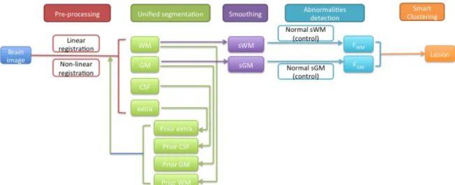
MRI images such as T1-weighted or T2-weighted images have been widely used for structural segmentation and pathology recognition in the brain because of their high sensitivities for different kinds of tissues. Here, we developed a pipeline, which is compatible for both modalities to automatically identify lesions based on the Automatic Lesion Identification toolbox (ALI) created by Seghier and colleagues (Seghier et al. 2008). This package is embedded in SPM12 software (Wellcome Trust Centre for Neuroimaging, London, UK, http://www.fil.ion.ucl.ac.uk/spm/) and it uses a multi-step approach to segment the lesions. The ALI toolbox has a linear spatial registration (Talairach and Tournoux 1988) implemented yet we chose to add a non-linear transformation to register the brain images of healthy subjects and stroke subjects for a more robust alignment which should also lead to improved accuracy of lesion detection. After obtaining the initial lesion result from ALI toolbox, we then added a smart clustering algorithm to greatly increase the true positives and decrease the false negatives. A schematic of the method is shown in Figure 1.1.
Figure 1.1 Schematic graph of automatic segmentation
4
A database (Corbetta et al. 2015) containing the MRI images of 132 stroke patients was used. The stroke patients were recruited from the stroke service at Barnes-Jewish Hospital (BJH), with the help of the Washington University Cognitive Rehabilitation Research Group (CRRG)(Dr. Lisa Connor) from 5/1/2008 to 5/30/2013. Data was collected in the stroke subjects at 3 time points (acute: 2 weeks after stroke, chronic1: 3 months after stroke, chronic2: 1 year after stroke) and included MRI scans (T1, T2, and FLAIR), resting state functional MRI and a large battery of behavioral measures. A healthy subject group (N = 45) is use as controls on whom the same data was collected at two time points 3 months apart. The subjects in the healthy control group are matched with the study sample for age, gender and years of education.
Scanning was performed using Siemens 3T Tim-Trio scanner and the standard 12-channel head coil at the Washington University School of Medicine. The two structural scans include a sagittal MP-RAGE T1-weighted image (TR=1950 msec, TE=2.26 msec, flip angle=9 degree, voxel size=1.0×1.0×1.0 mm, slice thickness=1.00 mm) and a transverse turbo spin-echo T2-weighted image (TR=2500 msec, TE=435 msec, voxel size=1.0×1.0×1.0 mm, slice thickness=1.00 mm) (Corbetta et al. 2015).
1.2.2 Preprocessing
T2-weighted images are registered to T1-weighted images using a cross-modal process based on the alignment of image intensity gradient (Rowland et al. 2005). Then the images are transformed into atlas-space (Talairach and Tournoux 1988) through a 12-parameter affine transformation, linearly registering the whole brain to a similar size, shape and orientation. Linear registration can only rotate, zoom and shear one image to match a common space by linear deformation. This allows for the whole size of brain match with each other in the images, some local areas such as sulci and gyri within the brain vary. To make the brain images more consistent, a non-linear registration is performed through FSL (Analysis Group, FMRIB, Oxford, UK, http://fsl.fmrib.ox.ac.uk/fsl/fslwiki/) to permit local deformations. Since some stroke patients have enlarged ventricles and which is quite unusual in healthy subject, directly comparing the images of
5
the above two will result in identifying the abnormal ventricle as lesion. Nonlinear registration is thus used to remove the influence of abnormal tissues that are not lesions. SPM was used to mask out areas outside of the brain in the aligned image, and to smooth and apply bias correction (Ashburner and Friston 2005) to reduce the effect of intensity inhomogeneity caused by MRI settings and the patients’ position.
1.2.3 Unified segmentation
The ALI toolbox (Seghier et al. 2008) in SPM12 was used for the segmentation of the lesions. The first step is to separate the voxels into white matter (WM), grey matter (GM) and cerebrospinal fluid (CSF). This step combined with bias correction is implemented using the commands in ALI toolbox to generate a probabilistic modal, which is used for subject-specific classification in SPM (for more details see Ashburner and Friston 2005). The brain images of healthy subjects are segmented into the above three groups based on the prior intensity information of WM, GM and CSF from predefined priors, which were previously created as templates based on 452 healthy controls (International Consortium for Brain Mapping, http://www.loni.ucla.edu/ICBM/). Each prior defines the probability of a voxel belonging to a category. The voxels is assigned to the category with which it has the highest likelihood, which is based on the intensity and the probability. However, abnormal tissues (eg. lesions) cannot reliably classify into one of the three categories. For example, a lesion in a T1-weighted image can have the intensity of grey matter where normally white matter exists, causing a mismatch between spatial and intensity information. Therefore, voxels that have a low probability in the three categories are put in a fourth group. Since the usually misclassified voxels often appear within WM, the ALI toolbox calculates the general extra group criteria for first use based on the prior intensity information of WM and CSF:
𝑮𝒆𝒙𝒕𝒓𝒂 =𝑮𝑾𝑴!𝑮𝟐 𝑪𝑺𝑭 (1.1)
Where GWM and GCSF are standard probabilities of WM and CSF in normal brain. Using equation 1.1 as a prior to define the extra group, this fourth group consists of subject specific abnormal voxels. Subsequently, the procedure of classifying the brain into different groups is implemented again,
6
including this newly formed extra group (after a refinement that removes the extra group voxels with a probability below one third) as a prior to increase the accuracy of classification, especially for the lesion voxels whose intensity is in the range of WM and GM (Seghier et al. 2008). After this second iteration, the resulting WM and GM maps are smoothed using a Gaussian kernel of 8mm full-width-at-half-maximum (FWHM), to create separate image files of WM and GM for the use in the next step in which the lesion is identified. This process is performed on each of our patients and controls.
1.2.4 Abnormalities detection
In MRI images the image contrast is a function of tissue density, measuring the proton density. In T1-weighted images, the intensities of one type tissue are consistent because of their similar constitution while tissues with higher fat content such as white matter are brighter than grey matter tissue (Koenig et al. 1990). The difference of intensities in image caused by the above property can be used to detect of abnormal tissues in the brain through Fuzzy Clustering with fixed Prototypes (FCP) (for more details, see (Seghier, Friston, and Price 2007)). This time we are using our own age matched healthy subjects to compare the patients. Using the maps created in the previous step, fuzzy sets representing the probability WM and GM are formed containing WM and GM of all control subjects as well as the target patient. First, to identify the white matter abnormal tissue of the patient, the intensity of voxel n (n = 1,2,…,Nvoxel) in WM for one subject (the patient or a control
subject) j (j = 1,2,…, Nsub) in the fuzzy set is compared with the mean value of voxel n in the WM
fuzzy set. A similarity metric Snj is used to quantify the difference for voxel n in subject j: 𝑺𝒏𝒋 = 𝟏−𝐭𝐚𝐧𝐡 (𝑵𝑵𝒔𝒖𝒃
𝒔𝒖𝒃!𝟏× 𝑿𝒏𝒋!𝑿𝒏
𝜶 ) (1.2)
Where 𝜶 is a constant “tuning” parameter and tanh is the hyperbolic tangent. 𝑿𝒏𝒋 is the value of j-th
subject at voxel n and 𝑿𝒏 is the mean value of voxel n over all subjects in the fuzzy set. Furthermore, this similarity metric Snj is used to quantify the degree of membership Mnj of voxel n to
7 𝑴𝒏𝒋 =
𝑺𝒏𝒋𝝀
𝑺𝒏𝒋𝝀
𝒋 (1.3)
Where 𝝀 is another tuning parameter. Subsequently, when j indexes the patient and the value of Mnj
is lower than threshold T, the n-th voxel is defined as a part of the lesion set FWM, which contains the
voxels that have a low probability in WM (even though it is spatially within WM) for this patient. The same procedure is repeated to get the fuzzy set FGM for the grey matter. Finally, the two sets
FWM and FGM are unified and voxels that have a low probability for either WM or GM are identified
as abnormal.
1.2.5 Post-processing: clustering
Using this method we obtained the initial lesion results by extracting the abnormal tissue. However, the human brain is highly variable even in healthy subjects the consistently appearing gyri and sulci exhibit pronounced variability in size and configuration (Thompson et al. 1996), thus this method resulted in a high number of false positives. Using a default threshold (T = 0.3) of fuzzy degree of membership M (M= [0,1]) to decide whether the voxel is part of the lesion gave highly varied results. Figure 1.2 shows the result using a default threshold, which in this case leads to incomplete lesion
identification. Figure 1.3 (a) shows a case where the lower threshold leads to false positives.
8
We chose to implement a smart clustering method with varying thresholds (ranging from 0 to 1) to improve the identification of the final lesion. Cluster is a gathering of voxels and is defined by similar intensities. If a low threshold is used, multiple clusters are found including many false positives (Figure 1.3 (a)); with a strict threshold only parts of the lesion are identified (Figure 1.3 (b)).
Figure 1.3 Lesion results with: (a) T = 0.08 without clustering; (b) T = 0.4 without clustering
By analyzing the lesion results at low and high thresholds, we realized that the difference between the center of the real lesion and normal tissue is larger than that between false positives and normal tissues. Therefore, we developed a smart clustering algorithm to combine the lesion results generated by different thresholds. We first identified a single lesion cluster x that covers the most distinctive part of the real lesion by setting a strict threshold (T = 0.4). This cluster x is however likely not covering the full extent of the lesion. This cluster is subsequently used to find the correct lesion cluster in lesion files generated by multiple less strict thresholds. For each of these files we extract the five largest size clusters (y1, y2, y3, y4, y5), which are the ones that most likely cover the real
lesion, and calculate intersection between every cluster yi (i = 1,2,3,4,5) with the strict cluster x, in
each lesion file. Using this method we can find the particular cluster yrealwhose intersection with x is
not zero and identify this cluster yreal as the actual lesion and the others as noise. With this method
we can identify the cluster that is most likely the real lesion for different thresholds, with a cluster that is more likely to cover the extent of the lesion.
9
Finally, since the segmented lesion is in the template space, we need to transform it into its own space for further study. During registration the local regions are non-linearly matched to the template and the relative locations of these regions within brain have been altered. Since the location of a lesion is as important as the size of a lesion, the lesion is transformed back to its own space for accurate spatial information. The method to implement the re-transformation is done by applying the warp file that we obtained when we employ the nonlinear registration to the generated lesion file.
1.2.6 Interface pipeline
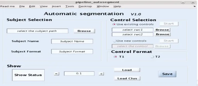
To make these steps user friendly, we developed an automatic segmentation interface that combines the function of the above steps and includes a module to view results with a point and click graphical user interface (GUI) (Matlab, The Mathworks Inc., Natick, MA, USA). With the high variability between patients and lesions, setting a single threshold did not give the best results. This interface allows users to view and compare the different identified lesion results, and make the final decision to extract the real lesion. The automatic segmentation interface (Figure 1.4) is divided into three parts: Subject Selection, Control Selection and Show.
10
Subject selection: here the structural image of the patient is selected. Either T1-weighted or T2-weighted 4dfp images can be entered.
Control selection: here the control images are selected. For the first use, “Use new controls” should be selected to enter the healthy subjects’ brain image. By doing so, all the control subjects will go through the preprocessing, unified segmentation steps as the target patient image. For the second use, since the needed fuzzy set of WM and GM for control group have already been built, user can choose “Use existing controls” at this point, which will save a lot of time by escaping preprocessing and unified segmentation steps. Note: T1-weighted subjects can only be compared with control subjects’ T1-weighted images.
Show: after beginning lesion identification by click on “Start” button, the small window in the “Show” panel will present the working status by changing from “Processing” to “Complete ALI”. After analyzing the patient data versus the controls the user can use the interface to visually check the results by viewing the lesion overlay on the initial brain image with a separate initial brain image next to it (Figure 1.5). By changing the threshold value through “+” and “-” button and press “Load Clus” or “Load” to choose implementing the smart clustering or not, the user can view the results at different thresholds in the viewing window. After finishing all the comparisons, the “Save” button is used to only obtain the selected lesion file and remove the others (to save space and simplify files).
11
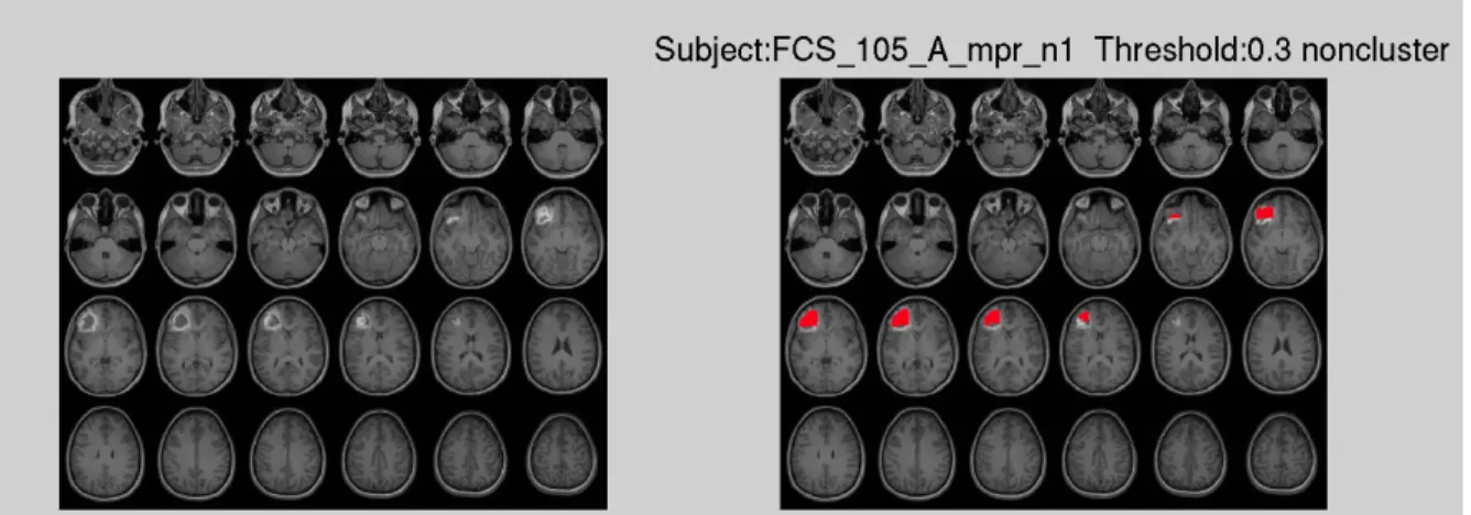
Figure 1.5 (a) Non-clustering result at threshold T = 0.1 for stroke patient 105 for T1 image
12
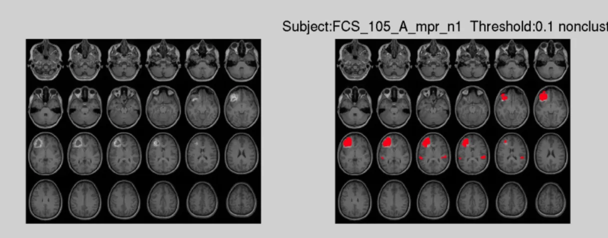
Figure1.6 (a) Non-clustering result at threshold T = 0.1 for stroke patient 105 for T2 image
Figure1.6 (b) Clustering result at threshold T = 0.1 for stroke patient 105 for T2 image
1.3
Results
In order to evaluate how the automatic lesion identification method works, the most direct way is to view the lesion result. Figure 1.5 and Figure 1.6 show the identified lesion generated at threshold 0.1 of T1-weighted image and T2-weighted image respectively, both with and without clustering.
The accuracy of the lesion identification method is evaluated by a Receiver Operating Characteristic (ROC) curve (Swets et al. 1979) and similarity index (Dice 1945). In order to test how the automatic segmentation works, we first manually segmented the target brain images for patients. We used the manually segmented lesions as a gold standard to evaluate the difference between the automatic and manually traced lesions.
ROC curves have been widely used in the radiologic community as a tool to visualize the accuracy of detecting Regions Of Interest (ROIs) using different thresholds. In an ROC curve the x-axis represents false positive fraction (FPF)/1-specificity and the y-axis represents the true positive fraction (TPF)/sensitivity. The ROC curve thus takes “hits” and “false alarms” into consideration,
13
providing an estimation of the overall accuracy. Thus, by looking at the shape of ROC curve we can evaluate the accuracy of this lesion identification method. If the ROC curve is closer to the top left,
Figure1.7 (a) Figure1.7 (b)
Figure 1.7 ROC curve for stroke subject 105: (a) without clustering (b) with clustering
the identified lesion is closer to the real lesion. Furthermore, calculating the area under curve (AUC) is another way to evaluate the ROC curve. The larger the AUC, the better the result. Two examples of the ROC curves for stroke patient 105 (Figure 1.7), without and with smart clustering.
From the ROC and AUC we can get an idea of the accuracy in this particular subject. However, it does not give us a quantitative measurement of which threshold generates the most reasonable lesion result for the subject. A similarity index is introduced to quantify the accuracy of detection. The similarity index is calculated as:
𝑺𝑰= 𝟐×𝑹𝒆𝒇!(𝑹𝒆𝒇∩𝑺𝒆𝒈𝑺𝒆𝒈) =𝟐×𝑻𝑷!𝑭𝑷!𝑭𝑵𝟐×𝑻𝑷 (1.4)
Where Ref represents the reference image (manual) and Seg represents the auto-segmented image. TP, FP and FN are the number of voxels that are true positive, false positive and false negative respectively. The value of similarity index ranges from 0 to 1 and the higher the value, the better the result. Thus we can compare the SI of different lesion results generated by different thresholds in one subject to decide which one works best.
14
However, SI also has its own limit on evaluating the accuracy. With the high proportion of true positive in the equation, SI focuses more on getting true positives rather than avoiding false positives. For example, although the similarity index of the lesion results for patient 105 in Figure 1.3 generated at threshold 0.1 without clustering and with clustering are 0.63 and 0.40 respectively, we might still want to choose the clustered result (lower SI) because of its low false. Therefore, it is best to use the value of the similarity index in combination with the ROC curve to find the best lesion result.
Figure 1.8 shows an overall result for all subjects without clustering and with clustering. Each dot on the graphs represents the best lesion result for each subject. It is obtained by extracting the lesion result that has highest SI under the condition of FPF less than 0.008 to ensure avoiding false positives. In general, we can see that implementing smart clustering can greatly decrease the FPF and increase TPF.
Figure 1.8 (a) Figure 1.8 (b)
Figure 1.8 For all subjects obtain the best lesion result: (a) without clustering (b) with clustering
Choosing the best result as mentioned above is however only possible in a set that has been manually segmented. In new patient data this lesion identification method is set to find multiple
15
solutions that are as close as possible to the ideal solution, but the user has to manually make the final decision using the GUI.
1.4
Discussion
By adding pre-processing and post-processing steps to the ALI toolbox, we developed a pipeline to automatically segment lesion in the brain. This method is compatible for T1 or T2-weighted images. Using the interface, user can conveniently segment and view the results within several clicks. And they can choose which lesion result is most reasonable. The user can then export the lesion result and load it in Analyze biomedical imaging software system ((Robb and Hanson 1991), Wideman-one.com/gw/brain/analyze/formatdoc.htm) to manually refine the result if necessary.
Lesion identification in ALI toolbox is based on finding abnormal tissue in patients as compared to healthy subjects. The high variability of human brains was the first problem we needed to solve in order to avoid identifying normal tissue as lesion, for example due to enlarged ventricles. We added a nonlinear registration that can align the inner regions of brain, e.g. normalizing abnormally enlarged ventricles. This allows for the treatment of the identified differences between healthy subjects and stroke subjects as likely being a part of the lesion.
By analyzing the results that are generated directly after comparison at a default threshold, we found that there was a trade off between identifying only part of the lesion (Figure 1.2) vs. identifying the whole lesion with the inclusion of false positive elsewhere. This trade-off is due to several factors. First, when the size of control group is limited, there is a chance that the range of normal tissue intensities is not well represented in the prior leading to the incorrect classification of that tissue as abnormal. The best way to solve this problem lies in increasing the size of the control group, and restricting other variables that can influence tissue intensity, such as age and gender, to increase the similarity of the control and the patient groups. The second problem occurs when cortical and subcortical structures show high inter-individual variability in size, orientation, topology and
16
geometric complexity (Thompson et al. 1996) that corresponds to gyral and sulcal geometry variability in the cortex. Obvious inter-subject variations have been reported in primary motor, somatosensory and auditory cortex (Missir et al. 1988; Rademacher et al. 1993), primary and associated visual cortex (Stensaas, Eddington, and Dobelle 1974), frontal and prefrontal areas (Selemon, Rajkowska, and Goldman-Rakic 1995). These problems are likely to inject false positives in the lesion classification. To improve accuracy and limit the influence of these variations we implemented a smart clustering algorithm to obtain the correct lesion cluster that covers as much of the lesion as possible. From Figure 1.7, we can see that clustering moves the ROC curve to the top-left indicating fewer false positive and more true positive after applying smart clustering.
Finally, to provide users more chances to only obtain the complete lesion, we create a user-friendly interface that not only incorporates all the steps, but also visualize flexibly their results for smarter decision. The users can easily view the lesions identified at different thresholds with and without smart clustering. Finally the user identifies the result that is closet to their needs and selects it, which can then be exported and manually edited if necessary. This process gives users more options and increases the accuracy to the best with lowest labor and time cost.
In our study, we assume the precisely manually identified lesion as a gold standard to generate ROC curve and calculate similarity index. After testing more than 100 stroke patients with both ischemic and hemorrhagic etiology, we find that the method works well for lesions located in white matter and grey matter and irrespective of their size. However, since the borders of lesions contain a mix of healthy tissues and damaged tissues, the intensity signal at the border shows less change than at the center (Stamatakis and Tyler 2005). Thus some borders still remain undetected such as in Figure 1.4(b). For small lesions in brainstem and cerebellum (less than 100 voxels), it is difficult to use this method to identify the lesions even with the smart clustering algorithm. Small lesion will have high variability of intensities at the border which decreases the accuracy of this method (Rademacher et al. 1993). Furthermore, as this method identifies the tissue contrast differences between control subjects and stroke subjects, it will regard all detected differences as lesion. For example,
17
periventricular white matter disease (PWMD) represents a common contrast changes observed in the periventricular white matter of aging subjects putatively due to small vessel damage (Filley 2012). If severe it can cause cognitive decline (Black, Gao, and Bilbao 2009). PWMD is identified as “lesion” using the this method. After applying the smart clustering algorithm, we can eliminate effectively these false positives. Interestingly, in future work this method could be used to identify the severity of white matter disease in subjects with or without lesions.
Future developments could include the use of multi-channel images to implement lesion
identification. Finding a way to efficiently combine the separate contrast information from different structural images can be of great potential. T1-weighted and T2-weighted image contrasts result from variation of relaxation time of protons (Hornak 2008), whereas other image modalities focus on different properties of tissues and should also be considered for combined lesion segmentation. For example, diffusion weighted image (DWI) map the magnitude of diffusion of molecules to generate image contrasts from the differences in diffusion rate. Another example is diffusion tensor image (DTI), which can be used to track the trajectory of fibers (WM). These methods could provide us with more information allowing for more accurate lesion identification.
18
Chapter 2
Spatial shift
s in cortical motor representations
post-stroke
2.1
Background
2.1.1
Mechanisms of reorganization
In the brain, the motor and somatosensory cortices are somatotopically organized where different regions represent different parts of the body in an organized fashion (the homunculus). Multiple animal and human studies have shown changes in sensory and motor representation after brain injury or amputation of limbs (Cramer and Crafton 2006; Randolph J. Nudo 2006; Kaas and Qi 2004). Interestingly, different changes in neural organization have been observed with different injury models. Two “canonical” injury models have been shown to change cortical representations: (1) peripheral nerve injury, and, 2) damage to the cerebrum itself, either subcortical or cortical (directly to the motor cortex).
The first kind of reorganization focuses on peripheral nerve injury such as limb amputation. This reorganization has been investigated both in humans and animals, and in different target regions: visual (Hubel and Wiesel 1970), somatosensory (Kaas 2000), olfactory (Wilson, Sullivan, and Leon 1987) and motor (Donoghue and Sanes 1987). In general, the lost of afferent input will generate an unresponsive zone in the brain. As time goes on, the regions around the representation of deafferented body parts will move into the “stump region” (that no longer has a function) leading to an expansion of the neural representation for the surrounding preserved body parts. There are also
19
local alterations of connections between the “stump region” and neighboring (preserved) regions with the formation of new connections through axonal or dendritic sprouting (Navarro, Vivó, and Valero-Cabré 2007; Kaas 2000; Kaas and Qi 2004). The functional consequences of this neural reorganization are not entirely clear. Stimulation of the “stump region” leads to peripheral responses of neighboring body parts which would suggest that the stump is now partially controlling non-deafferented body parts possibly through novel intracortical connections verified by bidirectional tracers and electrophysiological recording (Florence et al. 1998). The functional shift into the “stump region” (refocusing) is not limited to the motor system, visual deprivation also lead to a compensatory increase in the representation of selective somatosensory inputs, for example, somatosensory stimulation in blind people can activate parts of the visual cortex (Cohen et al. 1997). These changes are likely due to increased learning and training in the preserved somatosensory inputs after losing one input, supporting the idea that cortical organization is dynamically remapped during learning and experience (Donoghue, Hess, and Sanes 1996).
The second kind of reorganization focuses on central nervous system injury such as cerebral lesions. Cerebral lesions can directly damage the neurons, e.g. as in a lesion of motor cortex, while subcortical lesions can affect function by disrupting the connections from the motor cortical representation site to the body, e.g. as in a lesion of the cortico-spinal tract fibers. In both cases patients can present with an enlargement or shift of the limb representation in the cortical area to the surroundings(Randolph J. Nudo 2006; R. Chen, Cohen, and Hallett 2002).
After a cortical stroke the reorganization happens with neuroanatomical alterations in both adjacent and remote cortical tissues. Locally the functions of the lesioned area shift to peri-infarct regions (Randolph J. Nudo 2006), which means the surrounding regions will partially take over the function of the damaged one. Immediately after the stroke this shift occurs through unmasking of existing but inactive pathways and through the formation of new synapses (Fisher 1992; Ago et al. 2003). Over time axonal regeneration and sprouting, which are supported by sequential waves of expression of growth-promoting genes after a focal infarct in the motor cortex (Carmichael et al.
20
2005), play a role in consolidating this functional shift (R. Chen, Cohen, and Hallett 2002). Therefore both recruitment of existing pathways and generation of new connections between the damaged area and its surroundings make the shift of damaged representation possible.
Unlike after a cortical stroke, the damage caused by subcortical lesion can be more diffuse due to damage to white matter tracts, which might affect a larger cortical area. Although the actual mechanism of reorganization after subcortical stroke is still unclear, we think that in patients with some residual motor function, the changes caused by a subcortical lesion are similar to both mechanisms presented. Similar to complete deafferentiation the cortical regions representing the limb tested completely lose their effect. However, like in cortical lesions, there is no complete deafferentiation there are chances patients can re-gain control of the corresponding body parts by unmasking existing pathways and forming new connections with surrounding brain regions. Several studies have investigated the remapping after subcortical stroke but the results have been varied.
Neuroimaging (fMRI, PET) studies found that hand movements of the affected limb cause a posterior shift of the geometric center of cluster activation in ipsilesional sensorimotor cortex in patients with subcortical ischemic stroke (Pineiro et al. 2001; Calautti et al. 2003). Posterior displacement of sensorimotor responses was also demonstrated in a group of patients with multiple sclerosis and damage of the corticospinal tract (Lee et al. 2000), as well as in patients with spinal cord injury (Green et al. 1998). Thus a posterior displacement in motor (sensory) peak response could be an index of relative deafferentation of the motor cortex.
In contrast, a magnetoencephalography (MEG) study reported an ipsilesional activation shift along the medio-lateral axis of the hand region in a group of three subjects, and recruitment of regions outside of hand area in three other individuals (Altamura et al. 2007). In relation to recovery, a transcranial magnetic stimulation (TMS) experiment found that after subcortical stroke better motor outcome correlated with a larger stimulation area in the whole group of stroke subjects (N = 27),
21
and a correlation between motor outcome and map shift in a subgroup of subjects (N = 10) with normal corticospinal conduction (Thickbroom et al. 2004).
In summary, the brief review highlights that the human correlates of spatial shifts in motor representation demonstrated so clearly in animals studies are far from clear. Shift along medio-lateral axis may represent a shift within motor cortex possibly reflecting the recruitment of neighboring body part representations, while an anteroposterior shift might indicate the recruitment of nearby non-primary motor areas with direct corticospinal projections, such as premotor cortex or pre-central cortex or increased excitability of connections between these areas and primary motor cortex (Byrnes et al. 2001). The reasons behind this variability are many including variability of methods, small sample sizes with variable lesion location and size, motor impairment, etc.
In the second analysis of my thesis I will focus on the question of possibly remapping of cortical motor representations post-stroke. This study has several advantages over previous studies. First, the sample size (N = 132) is larger than that in other studies. Secondly, we use a method based on resting state fMRI that maps all the connections between one area and the rest of the brain, not just highlights the peak of motor activation. Thirdly, our strategy involves a signal, i.e. the inter-hemisphere correlation of the fMRI signal time series between the normal and the damaged precentral-postcentral region of the brain, which allows for a topographic mapping of possible shifts in representation, as well as recruitment of additional premotor or sensory regions.
2.1.2 Hypothesis
We plan to measure the inter-hemispheric temporal correlation, as known as functional connectivity (FC) of the fMRI signal measured at rest between the normal hand motor representation (knob region) and damaged pre-central/post-central region in a group of stroke patients with motor deficits. We hypothesize the inter-hemispheric FC will show acutely a spatial shift along anterior-posterior axis to other non-motor region, or a medial-lateral axis to nearby face or leg region because of the unmasking of existing but inactive pathways. This will allow to separate a mechanism based
22
on shift within the motor cortex versus recruitment of accessory premotor/sensory regions. As the newly unmasked the lateral connections are more diffuse, the intensity of the highest connectivity on the damaged hemisphere might decrease. Furthermore, we hypothesize that the extent of the spatial change will have a relationship with the severity of the damaged function.
During the recovery process, especially for patients who have recovered well from motor deficits, we hypothesize the formation of new connections that compensate for the damaged ones, and that may appear as a spatial shift of FC consistent with a chronic recruitment of cortical regions outside of motor cortex. Moreover, we hypothesize a positive correlation between motor outcome and the degree of cortical shift.
2.2 Methods
Functional MRI (fMRI) measures blood oxygenation level-dependent (BOLD) signal, which is an indirect measure influenced by variations in blood flow, blood volume, and oxygenation that are related to neuronal activity and metabolism (Kim and Ogawa 2012). To avoid confounds related to behavioral deficits, i.e. patients with different level of deficits may generate different levels of motor activation when moving their weak limb, we choose to use resting-state fMRI (rsfMRI), a method based on the temporal correlations of spontaneous BOLD signal fluctuations while subjects rest quietly in a scanner (Greicius et al. 2009). During resting state, it has been shown that homologous connections of left and right primary motor network are somatotopic organized and that corresponding regions are highly correlated (Van Den Heuvel and Pol 2010). During our data collection behavioral measures of motor, sensory, language and cognitive abilities were gathered. For the current work we chose a dedicated arm score to measure motor deficits. In addition, since previous studies (Grefkes and Fink 2011; Volz et al. 2014; Jang et al. 2014) as well as our own data show a clear correlation (p<0.05) between motor deficit and cortico-spinal tract (CST) damage, we also combine the extent of CST damage with the measures the motor function. The analyses were carried out using Connectome DataBase and Connectome Workbench (Human Connectome
23
Project, Washington University in St. Louis, http://www.humanconnectome.org/). The statistics were done using IBM SPSS statistics (Statistical Package for the Social Science, IBM corportation, Armonk, New York, US) and Matlab (The Mathworks Inc., Natick, MA, USA).
2.2.1 Data acquisition
We use rsfMRI scans from same database as indicated in 1.2.1, of 132 stroke patients and 27 healthy age-matched controls (AMC). Data was collected in the stroke patients at 3 time points (2 weeks, 3 months, 1 year after stroke respectively) and data of AMC subjects was obtained at 2 time points, 3 months apart. The functional MRI data underwent preprocessing steps demonstrated in Baldassarre (Antonello Baldassarre et al. 2014) and are as follows: 1) compensation for asynchronous slice acquisition using sinc interpolation; 2) elimination of odd/even slice intensity differences resulting from interleaved acquisition; 3) whole brain intensity normalization to achieve a mode value of 1000; 4) spatial realignment within and across functional MRI runs; 5) resampling to 3 mm3 voxels in atlas space including realignment and altas transformation in one resampling step. The behavioral scores were obtained from the database in 1.2.1 as well. The arm deficit score is measured using the ARAT (Action Research Arm Test) with a range of 0 to 1 (after normalization) while the composite score was derived from a number of measures of range of motion, strength as well as dexterity for both upper and lower extremity. A principle component analysis was used to reduce number of variables (Corbetta et al. 2015). The number of voxels damaged in CST was measured by multiplying the probabilistic map of cortico-spinal tract (CST) with the lesions. The tract probability map is generated using diffusion tensor image (DTI) from 40 healthy subjects (A Baldassarre et al. 2016).
2.2.2 Surface based registration
The majority of fMRI studies measure BOLD signals in a volume space, which means each voxel is registered to its actual anatomical 3-D position. We chose a more accurate method based on computerized cortical surface representations (Drury et al. 1996; Bruce Fischl et al. 1999; Van Essen et al. 2001; Wandell, Chial, and Backus 2000; Schwartz, Shaw, and Wolfson 1989), which allows for
24
surface registration and surface manipulations. This method is advantageous over volumetric approaches because each vertex on the surface is much more consistently aligned across individuals and has been transformed to a 2D surface that is not affected by re-sampling and spatial normalization. It is realized by inflating the brain into a sphere to retain the location of the sulci and gyri. Then registering the vertices of the single subject brain sphere to a template atlas sphere, which is then transformed back to a brain (Glasser et al. 2013). The surface based method contains more complete data and is more effective in reducing inter-subject variability (B Fischl, Sereno, and Dale 1999). Considering our large and varied subjects pool using a consistent criterion across individuals is especially important.
2.2.3 Seed-based approach
After obtaining the fluctuations of BOLD signal in certain time period of the whole brain, we defined a seed in the brain as the target region. In this study the rsfMRI approach is based on the observation that homotopic cortical regions are strongly connected in healthy subjects. The goal was therefore to compare the strength and spatial topography of homotopic motor connections from a seed region in the “hand knob” (Yousry et al. 1997) of the normal hemisphere to the contralateral pre-central/post-central regions. The hand knob in each hemisphere was identified on the atlas and can be seen in yellow in Figure 2.1. The identified vertices were then used to select this hand region in our patients and controls. Through visual inspection this seed area matched well in individual healthy subjects and stroke patients. Four example subjects are shown in Figure 2.2.
25
Figure 2.2 Atlas generated hand knob seeds overlay on 4 subjects (from top to bottom: healthy subject 004, 010, stroke patient 067, 168)
Seed correlation map was computed by extracting the time course for the seed and computing the correlation coefficient (Pearson r) between that time course and the time course from all other brain vertices. Then the Pearson correlations went through Fisher z-transform to generate z(r) seed map (Antonello Baldassarre et al. 2014). Here, the seed placed is placed in the undamaged hemisphere to
26
generate correlation maps of both the undamaged and damaged hemisphere. Then it can be used to evaluate the location and intensity of highest correlation in the lesion-affected hemisphere, which we assume to be the new hand representation.
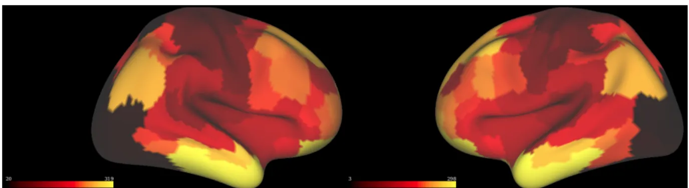
Figure 2.3 is the correlation map of control subject 003 for the left and right hemispheres when the seed, which marked in green, is placed on the left hemisphere. The colors of the brain surface represent the correlation value with respect to the seed. Regions in yellow have stronger temporal correlation with the hand knob region.
Figure 2.3 Left and right hemisphere correlation maps for control subject 003
To reduce noise (and the number of comparisons) we limit our search region to the area around the central sulcus. The parcelation of Gordon et al (Figure 2.4) was used to select the parcels of the pre and post central gyrus (Gordon et al. 2014).
27
We extracted the regions that cover the pre and post central gyrus and make a central sulcus mask that contains 982 vertices, as shown in Figure 2.5(a). Figure 2.5(b) shows the central sulcus correlation map for control subject 003 after applying this mask on the right hemisphere.
Figure 2.5 (a) Central sulcus mask Figure 2.5 (b) Central sulcus correlation map for control subject 003
2.2.4 Peak analysis
After obtaining the region map within the central sulcus on the damaged hemisphere, the first method to analyze the spatial shift of the sensorimotor region is to implement a peak analysis. This method identifies vertex within the mask that has the highest correlation with our seed in the undamaged hemisphere. To decrease fining local maxima that are caused by noise we clustered the correlation maps and identified the vertex with the highest correlation within the largest cluster. To cluster the data, we first normalized the vertices in central sulcus region to generate a z-scored correlation map (mean = 0; standard deviation = 1). Then we sorted the vertices of this z-scored map according to their correlation intensities in ascending order. We extracted the correlation value of the 99% percentile in this map and delete the vertices whose correlation intensity is below this correlation value. The remaining vertices are the ones with the highest 5% correlation value in the central sulcus. Next, we clustered those vertices using Human Connectome Workbench (Marcus et al. 2011) to separate the vertices into different groups based on their spatial location. After that, we picked the largest size cluster and define the peak vertex within this cluster as real peak vertex with respect to the hand knob on the undamaged hemisphere. At this point, we can use the index of this
28
vertex to get corresponding X, Y and Z coordinates (Talairach and Tournoux 1988) and evaluate the spatial change.
2.2.5 Region analysis
As a second analysis we investigated the intensity change around hand area in the damaged hemisphere, done through a region analysis in different groups (within stroke patients: motor deficit group and no deficit group). Instead of only analyzing the correlation value for one vertex, we generated a circle region around the real peak vertex with a radius of 2cm. Depending on the exact location this includes approximately 100 vertices. For each subject, the values within the sphere are binned to get the frequency of each value. Next, for all the subjects in a group (deficit or no deficit), the vertices within the circles are combined based on the ratio’s of the frequencies to correct for the different number of vertices for each subject and the size of groups. Thus instead of directly summing the times of occurrence for different intensity values, we calculate frequencies in each subject and combine them to get a distribution of the intensities in the circle for all the subjects in that group (finally divided by the number of subjects in the group) avoiding the influence of different vertex numbers in the circle for different subjects.
2.3 Results
The analysis of the spatial shift of peak vertex and the intensity change of the region surround peak vertex are done separately at the acute stage and during recovery, in order to investigate the changes shortly after stroke as well as the changes during recovery.
2.3.1 Acute stage
Acutely, changes in the brain were investigated two weeks after stroke. The images of patients with lesions in the left hemisphere are flipped (Left to Right) to align all lesions onto the right hemisphere. We then placed the seed in the undamaged left hemisphere and identified the peak
29
vertex in the right hemisphere for all subjects (both control and stroke) using the described peak analysis. Then for each subject we plotted its x (left, right), y (anterior, posterior), z (ventral, dorsal) coordinates of the peak vertices, which can be seen in (Figure 2.6).
Figure 2.6 (a) X-Y axis (b) X-Z axis (c) Y-Z axis Figure 2.6 Coordinates of peak vertices for healthy subjects (blue) and stroke patients (red)
Blue dots represent healthy subjects (AMC controls; N = 27) and red dots represent stroke patients (N = 127). From Figure 2.6 above we can see that the blue dots are in the center of the red dots population in each of the three directions. It directly shows the increased variance of the location of stroke patients’ peak coordinates compared to healthy subjects. When we ran independent samples t-test on these two groups along three directions, a significant difference is shown along the X axis ( df = 152, p = 0.008) while along Y axis (df = 152, p = 0.900) and Z axis (df = 152, p = 0.132) difference were not significant. Therefore, acutely after stroke there is a spatial shift of the peak coordinate of inter-hemispheric FC, especially along the primary motor cortex (X axis: medial-lateral) in the damaged hemisphere for stroke patients compared to healthy subjects. The
distribution (Figure 2.6(b)) suggests that the peak of the FC is located more medially and dorsally, as in a shift toward the leg representation from the original hand knob.
y
x
x
y
z
z
lateral medial dorsal dorsal medial ventral ventral30
The large difference of group size between the AMC and stroke group could bias the results and there is a higher chance that stroke patients’ brain images contain more noise than those of healthy subjects. Therefore, instead of using the AMC subjects as control group, we chose to form a new control group consisting of stroke patients who do not have motor deficits and no CST damage. Based on the ARAT behavioral score and the degree of CST damage, we categorized our stroke patients into two groups: motor deficit with CST damage (motor deficit group; N = 51), and no motor deficit with no CST damage (no motor deficit group; N = 41). Patients with lesions in the “hand knob” region, no motor score or CST damage were excluded. Table 2.1 shows the two groups’ peak vertices’ coordinates.
Table 2.1 Peak vertices’ coordinates comparison for motor deficit and no deficit
Peak vertices’
coordinates Group N Mean/mm
Standard Deviation (Std.) Std. Error mean X Motor deficit 51 26.22 13.42 1.88 No motor deficit 41 30.81 8.27 1.29 Y Motor deficit 51 -23.02 8.78 1.23 No motor deficit 41 -24.15 7.36 1.15 Z Motor deficit 51 60.07 10.72 1.50 No motor deficit 41 58.51 6.53 1.10
The peak vertices of the motor deficit group are more variable than the no deficit group, especially in the X and Z directions, which can be seen as the large difference of standard deviation. The independent sample t-test between these two groups showed a trending significant difference along X axis (df = 90, p = 0.058) while the other two directions did not (Y: df = 90, p = 0.512; Z: df = 90, p = 0.415). Therefore this analysis confirms that the acute FC peak in the damaged motor cortex is
31
shifted in the X direction (more medially) both as compared to healthy subjects and a group of stroke subjects without motor deficits. While analysis of peak locations using directional values seek for a consistent shift in a give direction, the variability of lesions that can cause more motor deficits and the observation of consistently higher variance in the stroke group led us to consider the possibility that motor deficits are associated with more variability in cortical motor representation. Therefore, next we measured whether high variance in the motor deficit group was a result of spatial shift away from the normal peak (independent of direction). We calculated an ideal peak vertex coordinate (34.29, -24.22, 56.50) in the damaged hemisphere by averaging all the healthy subjects’ peak vertex coordinates. Then we calculated the absolute distance away from the ideal peak for all the subjects. Figure 2.7 shows the motor deficit group in red and no deficit group in green.
Figure 2.7 (a) X-Y axis (b) X-Z axis (c) Y-Z axis Figure 2.7 Absolute distances of peaks away from ideal peak for motor deficit and no deficit subjects (green: no motor deficit, red: motor deficit)
The green dots (no motor deficit) are closer to the zero point than the red dots (motor deficit), indicating that a spatial shift away from the idea peak in the motor deficit group. Independent samples t-test on the absolute distance from ideal peak confirmed this impression: X axis (df = 90, p < 0.001), Y axis (df = 90, p = 0.050) and Z axis (df = 90, p = 0.001). To further test the difference of absolute distance away from ideal point for two groups, we performed a Permutation test on three axes respectively. First, the standard deviation of the two groups was calculated separately as