Detecting Deviating Data Cells
Peter J. Rousseeuw and Wannes Van Den BosscheDepartment of Mathematics, KU Leuven, Leuven, Belgium
ARTICLE HISTORY Received July Revised May KEYWORDS Cellwise outlier; Missing values; Multivariate data; Robust estimation; Rowwise outlier
ABSTRACT
A multivariate dataset consists ofncases inddimensions, and is often stored in annbyddata matrix. It is well-known that real data may contain outliers. Depending on the situation, outliers may be (a) undesirable errors, which can adversely affect the data analysis, or (b) valuable nuggets of unexpected information. In statistics and data analysis, the word outlier usually refers to a row of the data matrix, and the methods to detect such outliers only work when at least half the rows are clean. But often many rows have a few contaminated cell values, which may not be visible by looking at each variable (column) separately. We propose the first method to detect deviating data cells in a multivariate sample which takes the correlations between the variables into account. It has no restriction on the number of clean rows, and can deal with high dimensions. Other advantages are that it provides predicted values of the outlying cells, while imputing missing values at the same time. We illustrate the method on several real datasets, where it uncovers more structure than found by purely columnwise methods or purely rowwise methods. The proposed method can help to diagnose why a certain row is outlying, for example, in process control. It also serves as an initial step for estimating multivariate location and scatter matrices.
1. Introduction
Most datasets come in the form of a rectangular matrixXwith nrows anddcolumns, wherenis called the sample size andd the dimension. The rows ofXcorrespond to the cases, whereas the columns are the variables. Bothnanddcan be large, and it may happen that d>n. There exist many data models as well as techniques to fit them, such as regression and principal component analysis.
It is well-known that many datasets contain outliers. Depend-ing on the circumstances, outliers may be (a) undesirable errors, which can adversely affect the data analysis, or (b) valuable nuggets of unexpected information. Either way, it is important to be able todetectthe outliers, which can be hard for highd.
In statistics and data analysis, the word outlier typically refers to a row of the data matrix, as in the left panel of Figure 1. There has been much research since the 1960s to develop fit-ting methods that are less sensitive to such outlying rows, and that can detect the outliers by their large residual (or distance) from that fit. This topic goes by the name of robust statistics, see, for example, the books by Maronna, Martin, and Yohai (2006) and Rousseeuw and Leroy (1987).
Recently, researchers have come to realize that the outly-ing rows paradigm is no longer sufficient for modern high-dimensional datasets. It often happens that most data cells (entries) in a row are regular and just a few of them are anomalous. The first article to formulate the cellwise paradigm was Alqallaf et al. (2009). They noted how outliers propagate: given a fractionεof contaminated cells at random positions, the CONTACT Peter J. Rousseeuw [email protected]
Color versions of one or more of the figures in the article can be found online atwww.tandfonline.com/r/tech.
expected fraction of contaminated rows is
1−(1−ε)d (1)
which quickly exceeds 50% for increasingεand/or increasing dimensiond, as illustrated in the right panel ofFigure 1. This is fatal because rowwise methods cannot handle more than 50% of contaminated rows if one assumes some basic invariance prop-erties, see, for example, Lopuhaä and Rousseeuw (1991).
The two paradigms are quite different. The outlying row paradigm is about cases that do not belong in the dataset, for instance, because they are members of a different population. Its basic units are the cases, and if you interpret them as points in d-dimensional space they are indeed indivisible. But if you con-sider a case as a row in a matrix then it can be divided, into cells. The cellwise paradigm assumes that some of these cells deviate from the values they should have had, perhaps due to gross mea-surement errors, whereas the remaining cells in the same row still contain useful information.
The anomalous data cells problem has proved to be quite hard, as the existing tools do not suffice. Recent progress was made by Danilov (2010), Van Aelst, Vandervieren, and Willems (2012), Agostinelli et al. (2015), Öllerer, Alfons, and Croux (2016), and Leung, Zhang, and Zamar (2016).
Note that in the right panel ofFigure 1we do not know at the outset which (if any) cells are black (outlying), in stark contrast with the missing data framework. To illustrate the difficulty of detecting deviating data cells, let us look at the artificial bivariate (d=2) example inFigure 2. Case 1 lies within the near-linear
© Peter J. Rousseeuw and Wannes Van Den Bossche
This is an Open Access article. Non-commercial re-use, distribution, and reproduction in any medium, provided the original work is properly attributed, cited, and is not altered, transformed, or built upon in any way, is permitted. The moral rights of the named author(s) have been asserted.
Figure .The rowwise and cellwise outlier paradigms (black means outlying).
pattern of the majority, whereas cases 2, 3, and 4 are outliers. The first coordinate of case 2 lies among the majority of thexi1 (depicted as tickmarks under the horizontal axis) while its sec-ond coordinatex22is an outlying cell. For case 3, the first cell x31 is outlying. But what about case 4? Both of its coordinates fall in the appropriate ranges. Either coordinate of case 4 could be responsible for the point standing out, so the problem is not identifiable. We would have to flag the entire row 4 as outlying.
But now suppose that we obtain five more variables (columns) for these cases, which are correlated with the columns we already have. Then it may be possible to see thatx41perfectly agrees with the values in the new cells of row 4, whereas x42 does not. Then we would conclude that the cellx42is the cul-prit. Therefore, this is one of the rare situations where a higher dimensionality is not a curse but can be turned into an advan-tage. In fact, the method proposed in the next section typically performs better when the number of dimensions increases.
This example shows that deviating data cells do not need to stand out in their column: it suffices that they disobey the pattern of relations between this variable and those correlated
Figure .Illustration of bivariate outliers.
with it. Here, we propose the first method for detecting deviat-ing data cells that takes the correlations between the variables into account. Unlike existing methods, ourDetectDeviatingCells (DDC) method is not restricted to data with over 50% of clean rows. Other advantages are that it can deal with high dimensions and that it provides predicted values of the outlying cells. As a byproduct it imputes missing values in the data. For software availability, seeSection 8.
2. Brief Sketch of the Method
The (possibly idealized) model states that the rowsxiwere gen-erated from a multivariate Gaussian distribution with unknown d-variate meanμand positive semidefinite covariance matrix, after which some cells were corrupted or became missing. How-ever, the algorithm will still run if the underlying distribution is not multivariate Gaussian.
The method uses various devices from robust statistics and is described more fully inSection 4. We only sketch the main ideas here. The method starts by standardizing the data and flagging the cells that stand out in their column. Next, each data cell is predicted based on the unflagged cells in the same row whose column is correlated with the column in question. Finally, a cell for which the observed value differs much from its predicted value is considered anomalous. The method then produces an imputed data matrix, which is like the original one except that cellwise outliers and missing values are replaced by their predicted values. The method can also flag an entire row if it contains too much anomalous behavior, so that we have the option of downweighting or dropping that row in subsequent fits to the data.
This method looks unusual but it successfully navigates around the many pitfalls inherent in the problem, and worked the best out of the many approaches we tried. Its main feature is the prediction of individual cells. This can be characterized as a locally linear fit, where “locally” is not meant in the usual
sense (of Euclidean distance) but instead refers to the space of variables endowed with a kind of correlation-based metric.
Along the way DDC imputes missing data values by their predicted values. This is far less efficient than the EM algo-rithm of Dempster, Laird, and Rubin (1977) when the data are Gaussian and outlier-free, but it is more robust against cellwise outliers.
The DDC method has the natural equivariance properties. If we add a constant to all the values in a column ofX, or multi-ply any column by a nonzero factor, or reorder the rows or the columns, the result will change as expected.
3. Examples
The first dataset was scraped from the website of the British tele-vision show Top Gear by Alfons (2016). It contains 11 objectively measured numerical variables about 297 cars. Five of these vari-ables (such as Price) were rather skewed so we logarithmically transformed them.
The left panel of Figure 3 shows the result of applying a simple univariate outlier identifier to each of the columns of this dataset separately. For columnj, this method first computes a robust locationmj(such as the median) of its values, as well
as a robust scalesjand then computes the standardized values
zi j=(xi j−mj)/sj. A cell is then flagged as outlying if|zi j|>c
where the cutoffc=2.576 corresponds to a tolerance of 99% so that under ideal circumstances about 1% of the cells would be flagged. Most of the cells were yellow, indicating they were not flagged. Here, we only show some of the more interesting rows out of the 297. Deviating cells whosezi jis positive are colored
red, and those with negativezi j are in blue. Missing data are
shown in white and labeled NA (from “Not Available”).
The right-hand panel ofFigure 3shows the corresponding cell map obtained by running DetectDeviatingCells on these data. In the algorithm, we used the same 99% tolerance setting yielding the same cutoffc=2.576. The color of the deviating cells now reflects whether the observed cell value is much higher or much lower than the predicted cell value.
The new method shows much more structure than looking by column only. The high gas mileage (MPG) of the BMW i3 is no longer the only thing that stands out, and in fact it is an electric vehicle with a small additional gasoline engine. The columnwise method does not flag the Corvette’s displacement, which is not that unusual by itself, but it is high in relation to the car’s other characteristics. None of the properties of the Land Rover Defender (an all-terrain vehicle) stand out on their own, but their combination does. The weight of 210 kg listed for the Peugeot 107 is clearly an error, which gets picked up by both methods. The univariate method only flags the height of the Ssangyong Rodius, whereas DetectDeviatingCells also notices that its acceleration time of zero seconds from 0 to 62 mph is too low compared to its other properties, and in fact it is physically impossible.
As a second example we take the Philips dataset, which measuresd=9 characteristics ofn=677 TV parts created by a new production line. The left panel ofFigure 4is a rotated version ofFigure 9(a) in Rousseeuw and Van Driessen (1999) and shows, from top to bottom, the robust distance RDi for
i=1, . . . ,n. These were computed as
RDi= (xi−T)S−1(xi−T), 31.5 33.8 16.7 68.5 17.7 26.8 26.1 28.2 24.7 82.9 19.8 9.3 38.2 14.3 18 12 20.1 1968 647 1991 6162 1368 1997 2199 2198 2191 2987 1598 998 2706 1461 1998 1328 1598 177 170 125 437 160 140 150 122 150 211 184 68 265 90 155 84 105 280 184 221 424 169 250 258 265 280 398 192 70 206 162 265 81 184 8.2 7.9 10.3 4.3 7.4 10.6 9.7 14.7 9.4 9.1 6.9 14.2 5.8 12 0 14.1 10.7 143 93 122 186 131 118 118 90 122 108 143 100 164 112 105 87 119 61 470 51 21 43 53 50 25 54 25 48 65 34 88 38 39 74 1480 1315 1427 1460 1075 NA 1653 2120 1605 2500 NA 210 1310 1071 2059 1158 1295 4701 3999 4597 4435 3660 4524 4570 4785 4555 4662 3734 3430 4374 4062 5125 3665 4255 1826 1775 1788 1844 1630 1838 1820 1790 1840 1760 1683 1630 1801 1731 1915 1645 1799 1477 1578 1477 1246 1490 1702 1685 1790 1710 1951 1378 1465 1282 1448 1845 1705 1452 Pr ice Displacement BHP To rq u e Acceler ation T opSpeed MPG W e ight
Length Width Height
By column 31.5 33.8 16.7 68.5 17.7 26.8 26.1 28.2 24.7 82.9 19.8 9.3 38.2 14.3 18 12 20.1 1968 647 1991 6162 1368 1997 2199 2198 2191 2987 1598 998 2706 1461 1998 1328 1598 177 170 125 437 160 140 150 122 150 211 184 68 265 90 155 84 105 280 184 221 424 169 250 258 265 280 398 192 70 206 162 265 81 184 8.2 7.9 10.3 4.3 7.4 10.6 9.7 14.7 9.4 9.1 6.9 14.2 5.8 12 0 14.1 10.7 143 93 122 186 131 118 118 90 122 108 143 100 164 112 105 87 119 61 470 51 21 43 53 50 25 54 25 48 65 34 88 38 39 74 1480 1315 1427 1460 1075 NA 1653 2120 1605 2500 NA 210 1310 1071 2059 1158 1295 4701 3999 4597 4435 3660 4524 4570 4785 4555 4662 3734 3430 4374 4062 5125 3665 4255 1826 1775 1788 1844 1630 1838 1820 1790 1840 1760 1683 1630 1801 1731 1915 1645 1799 1477 1578 1477 1246 1490 1702 1685 1790 1710 1951 1378 1465 1282 1448 1845 1705 1452 Volkswagen Golf Suzuki Jimny Ssangyong Rodius Renault Clio Porsche Boxster Peugeot 107 Mini Coupe Mercedes−Benz G Mazda CX−5 Land Rover Defender
Honda CR−V Ford Kuga Fiat 500 Abarth Corvette C6 Chevrolet Cruze BMW i3 Audi A4 Pr ice Displacement BHP To rq u e Acceler ation T opSpeed MPG W e ight
Length Width Height
DetectDeviatingCells
Figure .Selected rows from cell maps of Top Gear data: (left) when detecting anomalous data cells per column; (right) when using the proposed method.
661 − 675 646 − 660 631 − 645 616 − 630 601 − 615 586 − 600 571 − 585 556 − 570 541 − 555 526 − 540 511 − 525 496 − 510 481 − 495 466 − 480 451 − 465 436 − 450 421 − 435 406 − 420 391 − 405 376 − 390 361 − 375 346 − 360 331 − 345 316 − 330 301 − 315 286 − 300 271 − 285 256 − 270 241 − 255 226 − 240 211 − 225 196 − 210 181 − 195 166 − 180 151 − 165 136 − 150 121 − 135 106 − 120 91 − 105 76 − 90 61 − 75 46 − 60 31 − 45 16 − 30 1 − 15 X1 X2 X3 X4 X5 X6 X7 X8 X9 DetectDeviatingCells
Figure .Left: robust distances of the rows of the Philips data. Right: map of
Detect-DeviatingCellson these data, combined per blocks of rows.
where T and S are the estimates of location and scatter obtained by the minimum covariance determinant (MCD) from (Rousseeuw1985), a rowwise robust method. It shows that the process was out of control in the beginning (roughly rows 1– 90) and near the end (around rows 480–550). However, by itself this does not yet tell us what happened in those products.
In the right panel, we see the cell map of DDC. The analysis was carried out on all 677 rows, but to display the results we cre-ated blocks of 15 rows and 1 column. The color of each cell is the “average color” over the block. The resulting cell map indicates that in the beginning variable 6 had lower values than would be predicted from the remaining variables, whereas the later out-liers were linked with lower values of variable 8. (In between, the cell map gives hints about some more isolated deviations.) We do not claim that this is the complete answer, but at least it gives an initial indication of what to look for. (DDC also flagged some rows, but this is not shown in the cell map to avoid con-fusion.) Note that these data are not literally a multivariate sam-ple because the rows were provided consecutively, but both the MCD and DDC methods ignore the time order of the rows.
The next example is the mortality by age for males in France, from 1816 to 2010 as obtained from the Human Mortality Database (2015). An earlier version was analyzed by Hyndman and Shang (2010). Each case corresponds to the mortalities in a given year. The left panel in Figure 5 was obtained by ROBPCA (Hubert, Rousseeuw, and Vanden Branden2005), a rowwise robust method for principal component analysis. Such a method can only detect entire rows, and the rows it has flagged
are represented as black horizontal lines. A black row does not reveal any information about its cells. The analysis was carried out on the dataset with the individual years and the individual ages, but as this resolution would be too high to fit on the page, we have combined the cells into 5×5 blocks afterward. The combination of some black rows with some yellow ones has led to gray blocks. We can see that there were outlying rows in the early years, the most recent years, and during two periods in between.
By contrast, the right panel inFigure 5identifies a lot more information. The outlying early years saw a high infant mortal-ity. During the Prussian war and both world wars there was a higher mortality among young adult men. And in recent years mortality among middle-aged and older men has decreased sub-stantially, perhaps due to medical advances.
Our final example consists of spectra withd=750 wave-lengths collected on n=180 archeological glass samples (Lemberge et al. 2000). Here, the number of dimensions (columns) exceeds the number of cases (rows).
DetectDeviat-ingCellshas no problems with this, and the R implementation
took about 1 min on a laptop with Intel i7-4800MQ 2.7GHz processor for this dataset. The top panel inFigure 6shows the rows detected by the robust principal component method. The lower panel is the cell map obtained byDetectDeviatingCellson this 180×750 dataset. After the analysis, the cells were again grouped in 5×5 blocks. We now see clearly which parts of each spectrum are higher/lower than predicted. The wavelengths of these deviating cells reveal the chemical elements responsible.
In general, the result ofDetectDeviatingCellscan be used in several ways:
1. Ideally, the user looks at the deviating cells and whether their values are higher or lower than predicted, and makes sense of what is going on. This may lead to a bet-ter understanding of the data patbet-tern, to changes in the way the data are collected/measured, to dropping certain rows or columns, to transforming variables, to changing the model, and so on.
2. If the dataset is too large for visual inspection of the results or the analysis is automated, the deviating cells can be set to missing after which the dataset is analyzed by a method appropriate for incomplete data.
3. If no such method is available, one can analyze the imputed datasetXimpproduced byDetectDeviatingCells, which has no missings.
In 2 and 3, one has the option to drop the flagged rows before taking the step. If that step is carried out by a sparse method such as the Lasso (Tibshirani 1996; Städler, Stekhoven, and Bühlmann 2014) or another form of variable selection, one would of course look more closely at the deviating cells in the variables that were selected.
Remark.In the above examples, the cellwise outliers happened to be mainly concentrated in fewer than half of the rows, allow-ing the rowwise robust methods MCD and ROBPCA to detect most of those rows. This may give the false impression that it would suffice to apply a rowwise robust method and then to analyze the flagged rows further. But this is not true in general: by (1) there will typically be too many contaminated rows, so rowwise robust methods will fail.
2006 − 2010 2001 − 2005 1996 − 2000 1991 − 1995 1986 − 1990 1981 − 1985 1976 − 1980 1971 − 1975 1966 − 1970 1961 − 1965 1956 − 1960 1951 − 1955 1946 − 1950 1941 − 1945 1936 − 1940 1931 − 1935 1926 − 1930 1921 − 1925 1916 − 1920 1911 − 1915 1906 − 1910 1901 − 1905 1896 − 1900 1891 − 1895 1886 − 1890 1881 − 1885 1876 − 1880 1871 − 1875 1866 − 1870 1861 − 1865 1856 − 1860 1851 − 1855 1846 − 1850 1841 − 1845 1836 − 1840 1831 − 1835 1826 − 1830 1821 − 1825 1816 − 1820 0−4 5−9 10−14 15−19 20−24 25−29 30−34 35−39 40−44 45−49 50−54 55−59 60−64 65−69 70−74 75−79 80−84 85−89 By row 2006 − 2010 2001 − 2005 1996 − 2000 1991 − 1995 1986 − 1990 1981 − 1985 1976 − 1980 1971 − 1975 1966 − 1970 1961 − 1965 1956 − 1960 1951 − 1955 1946 − 1950 1941 − 1945 1936 − 1940 1931 − 1935 1926 − 1930 1921 − 1925 1916 − 1920 1911 − 1915 1906 − 1910 1901 − 1905 1896 − 1900 1891 − 1895 1886 − 1890 1881 − 1885 1876 − 1880 1871 − 1875 1866 − 1870 1861 − 1865 1856 − 1860 1851 − 1855 1846 − 1850 1841 − 1845 1836 − 1840 1831 − 1835 1826 − 1830 1821 − 1825 1816 − 1820 0−4 5−9 10−14 15−19 20−24 25−29 30−34 35−39 40−44 45−49 50−54 55−59 60−64 65−69 70−74 75−79 80−84 85−89 DetectDeviatingCells
Figure .Male mortality in France in –: (left) detecting outlying rows by a robust PCA method; (right) detecting outlying cells byDetectDeviatingCells. After the analysis, the cells were grouped in blocks of5×5for visibility.
n 1 1 d wavelengths glass samples By row n 1 1 d wavelengths glass samples DetectDeviatingCells
Figure .Cell maps ofn=180archeological glass spectra withd=750wavelengths. The positions of the deviating data cells reveal the chemical contaminants.
4. Detailed Description of the Algorithm
The DetectDeviatingCells (DDC) algorithm has been
imple-mented in R and Matlab (seeSection 8). As described before, the underlying model is that the data are generated from a multi-variate Gaussian distributionN(μ,)but afterward some cells were corrupted or omitted. The variables (columns) of the data should thus be numerical and take on more than a few val-ues. Therefore, the code does some preprocessing: it identifies the columns that do not satisfy this condition, such as binary dummy variables, and performs its computations on the remain-ing columns.
These remaining variables should then be approximately Gaussian in their center, that is, apart from any outlying values. This could be verified by QQ plots, and one could flag highly skewed or long-tailed variables. It is recommended to trans-form very non-Gaussian variables to approximate Gaussianity, like we took the logarithm of the right-skewed variable Price in the cars data inSection 3. More general tools are the Box–Cox and Yeo–Johnson (Yeo and Johnson2000) transformations that have parameters, which need to be estimated as done by Bini and Bertacci (2006) and Riani (2008). We chose not to automate this step because we feel it is best carried out by a person with sub-ject matter knowledge about the data. From here onward we will assume that the variables are approximately Gaussian in their center. The algorithm does not require joint normality of vari-ables to run.
The actual algorithm then proceeds in eight steps.
Step 1: standardization. For each columnjofX, we estimate mj=robLoci(xi j) and sj=robScalei(xi j−mj), (2)
where robLoc is a robust estimator of location, and robScale is a robust estimator of scale, which assumes its argument has already been centered. The actual definitions of these estimators are given in the Appendix. Next, we standardizeXtoZby
zi j =(xi j−mj)/sj. (3)
Step 2: apply univariate outlier detection to all variables. After the columnwise standardization in (3), we define a new matrix
Uwith entries
ui j=
zi j if|zi j|c
NA if|zi j|>c . (4)
Due to the standardization in (3), formula (4) is a columnwise outlier detector. The cutoff valuecis taken as
c=
χ2
1,p, (5)
where χ2
1,pis the pth quantile of the chi-squared distribution
with 1 degree of freedom, where the probability p is 99% by default so that under ideal circumstances only 1% of the entries gets flagged.
Step 3: bivariate relations. For any two variablesh= j, we compute their correlation as
corjh=robCorri(ui j,uih), (6)
where robCorr is a robust correlation measure given in the Appendix (the computation is over all ifor which neitherui j
oruihis NA). From here onward we will only use the relation
between variablesjandhwhen
|corjh|corrlim (7)
in which corrlim is set to 0.5 by default. Variablesjthat satisfy (7) for someh= jwill be calledconnected, and contain useful information about each other. The others are calledstandalone variables. For the pairs(j,h)satisfying (7) we also compute
bjh =robSlopei(ui j|uih), (8)
where robSlope computes the slope of a robust regression line without intercept that predicts variablejfrom variableh(see the Appendix). These slopes will be used in the next step to provide predictions for connected variables.
Step 4: predicted values. Next we compute predicted values ˆ
zi jfor all cells. For each variable jwe consider the setHj
con-sisting of all variableshsatisfying (7), including jitself. For all i=1, . . . ,n, we then set
ˆ
zi j=G({bjhuih; hin Hj}), (9)
whereGis a combination rule applied to these numbers, which omits the NA values and is zero when no values remain. (The lat-ter corresponds to predicting the unstandardized cell by the esti-mated location of its column, which is a fail-safe.) Our current preference forGis a weighted mean with weightswjh= |corjh|
but other choices are possible, such as a weighted median. The advantage of (9) is that the contribution of an outlying cellzihto
ˆ
zi jis limited because|uih|cand it can only affect a single term,
which would not be true for a prediction from a least-square multiple regression ofz.j on thed−1 remaining variablesz.h
together. We will illustrate the accuracy of the predicted cells by simulation inSection 5.
Step 5: deshrinkage. Note that a prediction such as (9) tends to shrink the scale of the entries, which is undesirable. We could try to shrink less in the individual termsbjhuih but this would
not suffice because these terms can have different signs for dif-ferenth. Therefore, we propose to deal with the shrinkageafter applying the combination rule (9). For this purpose, we replace ˆ
zi jbyajzˆi jfor alliand j, where
aj:=robSlopei(zij|ˆzij) (10)
comes from regressing the observedz.j on the (shrunk)
pre-dictedzˆ.j.
Step 6: flagging cellwise outliers. In Steps 4 and 5, we have com-puted predicted valueszˆi jfor all cells. Next we compute the
stan-dardized cell residuals ri j=
zi j− ˆzi j
robScalei(zij− ˆzij) .
(11) In each column jwe then flag all cells with|ri j|>cas
anoma-lous, wherecwas given in (5). We also assemble the “imputed” matrixZimp, which equalsZexcept that it replaces deviating cells zi j and NA’s by their predicted valueszˆi j. The unflagged cells
remain as they were.
We have the option of setting the flagged cells to NA and repeating steps 4 to 6 to improve the accuracy of the estimates. This can be iterated.
Step 7: flagging rowwise outliers. To decide whether to flag row i, we could just count the number of cells whose|ri j|exceeds a
cutoffa, but this would miss rows with many fairly large|ri j| <
a. The other extreme would be to compare avej(r2i j)to a
cut-off, but then a row with one very outlying cell would be flagged as outlying, which would defeat the purpose. We do something in between. Under the null hypothesis of multivariate Gaussian data without any outliers, the distribution of theri jis close to
standard Gaussian, so the cdf ofr2
i jis approximately the cdfFof χ2
1. This leads us to the criterion Ti= d ave j=1F r2 i j . (12)
We then standardize theTias in (3) and flag the rowsifor which
the standardizedTiexceed the cutoffcof (5).
When we find that rowihas an unusually largeTithis does
not necessarily “prove” that it corresponds to a member of a dif-ferent population, but at least it is worth looking into.
Even though theTican flagsomerowwise outliers, there are
types of rowwise outliers that it may not detect, for instance, in the barrow wheel configuration of Stahel and Mächler (2009) where a rowwise outlier may not have any largeri j2. Therefore, it
is recommended to use rowwise robust methods in subsequent analyses of the data, after dropping the rows that were flagged.
Step 8: destandardize. Next, we turn the imputed matrixZimp into an imputed matrixXimpby undoing the standardization in (3). The main output of DDC isXimptogether with the list of cells flagged as outlying and, optionally, the list of rowwise out-liers that were found.
Predicting the value of a cell in Steps 4 and 5 above evokes the imputation of a missing value, as in the EM algorithm of Dempster, Laird, and Rubin (1977). However, there are two reasons why the EM method may not work in the present situation. First of all, we would need estimators of location and scatterμˆ and ˆ that are robust against cellwise and rowwise outliers, which we only know how to obtain after detecting those outliers. And second, the conditional expectation ofxi jis
a linear combination of all the availablexihwithh= jbut some
of those cells may be outlying themselves, thus spoiling the sum. The DDC method employs measures of bivariate correlation, and regression for bivariate data. This may seem naive com-pared to estimating scatter matrices and/or performing multiple regression on sets ofq>2 variables. However, the latter would imply that we must compute scatter matrices betweenqvariables in an environment where a fractionεof cells is contaminated, so that according to (1) a fraction 1−(1−ε)qof the rows of length
qis expected to be contaminated. The latter fraction grows very quickly with q, and once it exceeds 50% there is no hope of estimating the scatter matrix by a rowwise robust method. So the largerqis, the less this approach can work. Therefore, we chose the smallest possible value q=2, which has the addi-tional advantage that the computaaddi-tional effort to robustly esti-mate bivariate scatter is much lower than for higherq.
To illustrate this,Table 1shows the effect of fitting substruc-tures in dimension q<d for various values of q. The total time complexity is the product of the time needed for a 50%-rowwise-breakdown fit (regression or scatter) to a q-variate dataset (in which elemental sets are formed byq−1 data points and the origin) and the number of combinations ofqout ofd variables (for larged). The complexity grows very fast withq. The next column is the expected breakdown value, that is, what
Table .Fitting substructures inq<ddimensions.
q Total time complexity Breakdown value Probability of cleanq-row∗
n dlog(d) .% .% n2d3 .% .% n3d4 .% .% n4d5 .% .% n9d10 .% .% n19d20 .% .%
NOTE:∗Assuming a % probability of a cell being outlying.
fraction of cellwise outliers at random positions these fits can typically withstand, that is, 1−2−1/q. The expected breakdown
value drops quickly withq. The final column is the probability that a subrow ofqentries contains no outliers when the prob-ability of a cell being outlying is 10%.Table 1is in fact overly optimistic because it does not account for the problem that the predictions from such q-variate fits are affected whenever at least one of the cells in it is outlying.
This should not be confused with the approach of Kriegel et al. (2009) who look for rowwise outliers under the assump-tion that outlyingness of a row is due to only a few variables whereas the other variables are deemed irrelevant. That situa-tion is different from both the general rowwise outlier setting and the cellwise outlier model, in each of which all variables may be relevant.
As described, the computation time (number of operations) of DDC is on the order ofO(nd2)due to computing alld(d− 1)/2 correlations between variables, where each correlation takesO(n)time. The required memory (storage) space is then alsoO(nd2). However, if the dimensiondis over (say) 1000, we switch to predicting each column by thekcolumns that are most correlated with it, thereby bringing down the space requirement toO(nd),which cannot be reduced further as it is proportional to the size of the data matrix itself. On a parallel architecture, we can reduce the computation time by letting each processor com-pute thekcorrelations for a subset of columns to be predicted. On a nonparallel system, we could switch to a fast approximate k-nearest neighbor method such as the celebrated algorithm of Arya et al. (1999), which would lower the computation time from O(nd2) to O(ndlog(d)). Compared to analyzing each column separately, this algorithm only spends an additional time factor log(d),which grows very slowly withd. A related speedup is used in Google Correlate (Vanderkam et al.2013).
5. Comparison to Other Detection Methods
We now compare DDC to a method that detects outlying cells per column, the univariate GY filter of Gervini and Yohai (2002) as described in (Agostinelli et al.2015). Applying the univariate GY filter to the columns of the cars data actually gives the same result as the simpler columnwise detection inFigure 3. The key difference between these methods is that the GY filter uses an adaptive cutoff rather than the fixed cutoff (5).
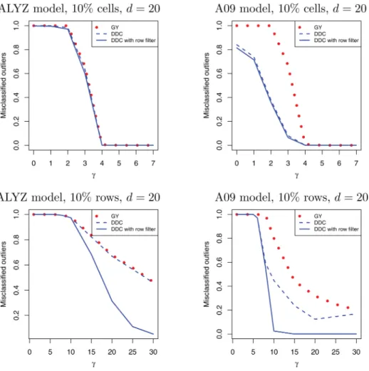
We will only report a small part of our simulations, the results of other settings being similar. First, clean multivariate Gaus-sian data were generated withμ=0and two types of covari-ance matrices with unit diagonal. The ALYZ (Agostinelli et al. 2015) random correlation matrices yield relatively low correlations between the variables, whereas the A09 correlation
matrix given by ρjh =(−0.9)|h−j| yields both high and low
correlations.
Next, these clean data were contaminated. Outlyingcellswere generated by replacing a random subset (say, 10%) of then×d cells by a valueγ, which was varied to see its effect.
Outlyingrowswere generated in the hardest direction, that of the last eigenvectorvof the true covariance matrix. Next we rescale v to the typical size of a data point, by making v−1v=E[Y2]=d where Y2∼χ2
d . We then replaced a
random set of rows ofXbyγv.
Figure 7shows the outlier misclassification rate (forn=200 and d=20). This is the number of cells that were generated as outlying and detected by the method, divided by the total number of outlying cells generated. This fraction depends on γ: it is high for smallγ (but those cells or rows are not really outlying) and then goes down. In the top panels, we see that all methods for detecting cells work about equally well when the correlations between variables are fairly small, whereas the new method does better when there are at least some higher correlations. The bottom panels show a similar effect for detecting rows, and indicate that using the row fil-ter, that is, Step 7 in Section 4, is an important component of DDC.
The same simulation yieldsFigure 8, which shows the mean squared error of the imputed cells relative to the original cell values (before any contamination took place), in which flagged rows were taken out. Again DDC does best when there are some
higher correlations. This confirms the usefulness of computing predicted cells in Step 4 of the DDC algorithm.
We have repeated the simulations leading toFigures 7and8 for dimensionsdranging up to 200,nbetween 10 and 2000, and contamination fractions up to 20%, each time with 50 replica-tions. The method does not suffer from high dimensions, and even forn=20 cases ind=200 dimensions the comparisons between these methods yield qualitatively the same conclusions.
6. Two-Step Methods for Location and Scatter
Now assume that we are interested in estimating the param-eters of the multivariate Gaussian distributionN(μ,)from which the data were generated (before cells and/or rows were contaminated).
If the data were clean, one would estimateμ andby the mean of the data and the classical covariance matrix. However, when the data may contain both cellwise and rowwise outliers, the problem becomes much more difficult. For this Agostinelli et al. (2015) proposed a two-step procedure called 2SGS, which is the current best method. The first step applies the univariate GY filter (from the previous section) to each column of the data matrixXand sets the flagged cells to NA. The second step then applies the sophisticated generalized S-estimator (GSE) of Danilov, Yohai, and Zamar (2012) to this incomplete dataset, yieldingμˆ andˆ. The GSE is a rowwise robust estimator ofμ andthat was designed to work with data containing missing
Figure .Outlier misclassification rates of different detection methods: (top) under cellwise contamination, (bottom) under rowwise contamination. Here GY is the Gervini– Yohai filter.
Figure .Mean squared error of the imputed cells in the same simulation.
Figure .LRT deviation of three estimates from the true scatter matrix.
values, following earlier work by Little (1988) and Cheng and Victoria-Feser (2002).
Our version of this is to replace GY in the first step by DDC, followed by the same second step. When the first step flags a row, we take it out of the subsequent computations. We also include the Huberized Stahel-Donoho (HSD) estimator of Van Aelst, Vandervieren, and Willems (2012), as well as the minimum covariance determinant (MCD) estimator (Rousseeuw 1985; Rousseeuw and Van Driessen1999), which is robust to rowwise outliers but not to cellwise outliers. For each method, we mea-sure how farˆ is from the trueby the likelihood ratio type deviation
LRT=trace(ˆ −1)−log(det(ˆ −1))−d
(which is a special case of the Kullback–Leibler divergence) and average this quantity over all replications.
Figure 9compares these methods in the same simulation set-tings asFigures 7and8. In the top panels, we see that the new method performs about as well as 2SGS when the correlations between the variables are fairly low, but does much better when there are some higher correlations. For rowwise outliers their performance is quite similar.
Agostinelli et al. (2015) showed that 2SGS is consistent, that is, it gets the right answer for data generated from the model without any contamination whenngoes to infinity. The proof follows from the fact that the fraction of cells flagged by the univariate GY filter goes to zero in that setting. This is not true for DDC because the cutoff value (5) is fixed, so some cells will still be flagged. Nevertheless the above simulations indicate that with actual contamination, using DDC in the first step often does better than GY.
A limitation of the GSE in the second step is that it requires n>dand in fact the dimensiondshould not be above 20 or 30, whereas the raw DDC method can deal with higher dimensions as we saw in the glass example withd=750.
7. Conclusions and Outlook
The proposed method detects outliers at the level of the indi-vidual cells (entries) of the data matrix, unlike existing out-lier detection methods, which consider the rows (cases) of that matrix as the basic units. Its main construct is the prediction of each cell. This turns a high dimensionality into a blessing instead of a curse, as having more variables (columns) available increases the amount of information and may improve the accu-racy of the predicted cells.
The new method requires more computation than consider-ing each variable in isolation, but on the other hand is able to detect outliers that would otherwise remain hidden as we saw in the first example. In simulations, we saw that DetectDeviat-ingCellsperforms as well as columnwise outlier detection when there is little correlation between the columns, whereas it does much better when there are higher correlations. Also, using it as the first step in the method of Agostinelli et al. (2015) outper-forms a columnwise start.
A topic for further research is to extend this work to nonnumeric variables, such as binary and nominal. For the interaction between numeric and nonnumeric variables, and
between nonnumeric variables, this necessitates replacing cor-relation by other measures of bivariate association. Also, for predicting cells the linear regression would need to be replaced by other techniques such as logistic regression.
8. Software Availability
The R code of theDetectDeviatingCellsalgorithm is available on CRAN in the packagecellWise, which also contains functions for drawing cell maps and allows to reproduce all the examples in this article. Equivalent MATLAB code is available from the websitehttp://wis.kuleuven.be/stat/robust/software.
Appendix: Components of the Algorithm
The building blocks of DetectDeviatingCells are some simple existing robust methods for univariate and bivariate data. Several are available, and our choice was based on a combination of robustness and compu-tational efficiency, as all four of them only requireO(n)computing time and memory.
For estimating location and scale of a single data column, we use the first step of an algorithm for M-estimators, as described on pages 39–41 of Maronna, Martin, and Yohai (2006). In particular, for estimating location we employ Tukey’s biweight function
W(t)= 1− t c 2 2 I(|t|c),
wherec>0 is a tuning constant (by defaultc=3). Given a univariate datasetY= {y1, . . . ,yn},we start from the initial estimates
m1= n med i=1(yi) and s1= n med i=1 |yi−m1|
and then compute the location estimate robLoc(Y)= n i=1 wiyi n i=1 wi , where the weights are given bywi=W((yi−m1)/s1).
For estimating scale, we assume thatYhas already been centered, for example, by subtracting robLoc(Y), so that we only need to consider devi-ations from zero. We now use the functionρ(t)=min(t2,b2)whereb=
2.5. Starting from the initial estimates2=medi(|yi|),we then compute the scale estimate robScale(Y)=s2 1 δ n ave i=1ρ yi s2 ,
where the constantδ=0.845 ensures consistency for Gaussian data. The next methods are bivariate, that is, they operate on two data columns, call themjandh. For correlation we start from the initial esti-mate ˆ ρjh= (robScalei(zi j+zih))2−(robScalei(zi j−zih))2 /4 (Gnanadesikan and Kettenring1972), which is capped to lie between−1 and 1 (this assumes that the columns of the matrixZwere already cen-tered at 0 and normalized). Thisρˆjhimplies a tolerance ellipse around (0,0) with the same coverage probabilitypas in (5). Then robCorr is defined as the plain product-moment correlation of the data points(zi j,zih)inside the ellipse.
For the slope, we again assume the columns were already centered, but they need not be normalized. The initial slope estimate is
bjh= n med i=1 z i j zih ,
where fractions with zero denominator are first taken out. For everyi, we then compute the raw residualri jh=zi j−bjhzih. Finally, we compute the
plain least-square regression line without intercept on the points for which |ri jh|c robScalei(rijh)wherecis the constant (5). We then define
robS-lope as the srobS-lope of that line.
Acknowledgments
The research of P. Rousseeuw has been supported by projects of Internal Funds KU Leuven. W. Van den Bossche obtained financial support from the EU Horizon 2020 project SCISSOR: Security in trusted SCADA and smart-grids 2015–1017. The authors are grateful for interesting discussions with Mia Hubert and the participants of the BIRS Workshop 15w5003 in Banff, Canada, November 16–20, 2015, and to Jakob Raymaekers for assistance with the CRAN packagecellWise. The reviewers provided helpful sugges-tions to improve the presentation.
References
Agostinelli, C., Leung, A., Yohai, V. J., and Zamar, R. H. (2015), “Robust Estimation of Multivariate Location and Scatter in the Presence of Cell-wise and CaseCell-wise Contamination,”Test, 24, 441–461. [1,7,8,10] Alfons, A. (2016), Package robustHD, R-Package Version 0.5.1, available at
http://CRAN.R-project.org/package=robustHD. [3]
Alqallaf, F., Van Aelst, S., Yohai, V., and Zamar, R. H. (2009), “Propagation of Outliers in Multivariate Data,”The Annals of Statistics, 37, 311–331. [1]
Arya, S., Mount, D. M., Netanyahu, N. S., Silverman, R., and Wu, A. Y. (1999), “An Optimal Algorithm for Approximate Nearest Neighbor Searching in Fixed Dimensions,”Journal of the ACM, 45, 891–923. [7]
Bini, M., and Bertacci, B. (2006), “Robust Transformation of Proportions Using the Forward Search,” inData Analysis, Classification and the For-ward Search, eds. S. Zani, A. Cerioli, M. Riani, and M. Vichi, New York: Springer, pp 173–180. [6]
Cheng, T. C., and Victoria-Feser, M. P. (2002), “High-Breakdown Estima-tion of Multivariate Mean and Covariance with Missing ObservaEstima-tions,” British Journal of Mathematical and Statistical Psychology, 55, 317–335. [10]
Danilov, M. (2010), “Robust Estimation of Multivariate Scatter in Non-Affine Equivariant Scenarios,” Ph.D. dissertation, University of British Columbia, Vancouver. [1]
Danilov, M., Yohai, V. J., and Zamar, R. H. (2012), “Robust Esti-mation of Multivariate Location and Scatter in the Presence of Missing Data,” Journal of the American Statistical Association, 107, 1178–1186. [8]
Dempster, A., Laird, N., and Rubin, D. (1977), “Maximum Likelihood from Incomplete Data via the EM Algorithm,”Journal of the Royal Statistical Society, Series B, 39, 1–38. [3,7]
Gervini, D., and Yohai, V. J. (2002), “A Class of Robust and Fully Efficient Regression Estimators,”The Annals of Statistics, 30, 583–616. [7] Gnanadesikan, R., and Kettenring, J. R. (1972), “Robust Estimates,
Resid-uals, and Outlier Detection with Multiresponse Data,”Biometrics, 28, 81–124. [10]
Hubert, M., Rousseeuw, P. J., and Vanden Branden, K. (2005), “ROBPCA: A New Approach to Robust Principal Component Analysis,” Techno-metrics, 47, 64–79. [4]
Human Mortality Database (2015),Human Mortality Database, Berke-ley: University of California; Max Planck Institute for
Demo-graphic Research. Available atwww.mortality.org(data downloaded in November 2015). [4]
Hyndman, R. J., and Shang, H. L. (2010), “Rainbow Plots, Bagplots, and Boxplots for Functional Data,”Journal of Computational and Graphical Statistics, 19, 29–45. [4]
Kriegel, H.-P., Kröger, P., Schubert, E., and Zimek, A. (2009), “Outlier Detection in Axis-Parallel Subspaces of High Dimensional Data,” in Lecture Notes in Computer Science(Vol. 5476), eds. T. Theeramunkong, B. Kijsirikul, N. Cersone, and T.-B. Ho, New York: Springer, pp 831– 838. [7]
Lemberge, P., De Raedt, I., Janssens, K. H., Wei, F., and Van Espen, P. J. (2000), “Quantitative Z-Analysis of 16th-17th Century Archaeologi-cal Glass Vessels using PLS Regression of EPXMA andμ−XRF Data,” Journal of Chemometrics, 14, 751–763. [4]
Leung, A., Zhang, H., and Zamar, R. (2016), “Robust Regression Esti-mation and Inference in the Presence of Cellwise and Casewise Contamination,” Computational Statistics and Data Analysis, 99, 1–11. [1]
Little, R. J. A. (1988), “Robust Estimation of the Mean and Covariance Matrix from Data with Missing Values,”Journal of the Royal Statisti-cal Society, Series C, 37, 23–38. [10]
Lopuhaä, H. P., and Rousseeuw, P. J. (1991), “Breakdown Points of Affine Equivariant Estimators of Multivariate Location and Covariance Matri-ces,”The Annals of Statistics, 19, 229–248. [1]
Maronna, R. A., Martin, R. D., and Yohai, V. J. (2006),Robust Statistics: The-ory and Methods, New York: Wiley. [1,10]
Öllerer, V., Alfons, A., and Croux, C. (2016), “The Shooting S-Estimator for Robust Regression,”Computational Statistics, 31, 829–844. [1] Riani, M. (2008), “Robust Transformations in Univariate and Multivariate
Time Series,”Econometric Reviews, 28, 262–278. [6]
Rousseeuw, P. J. (1985), “Multivariate Estimation with High Breakdown Point,” inMathematical Statistics and Applications(Vol. B), eds. W. Grossmann, G. Pflug, I. Vincze, and W. Wertz, Dordrecht: Reidel, pp. 283–297. [4,10]
Rousseeuw, P. J., and Leroy, A. M. (1987),Robust Regression and Outlier Detection, New York: Wiley. [1]
Rousseeuw, P. J., and Van Driessen, K. (1999), “A Fast Algorithm for the Minimum Covariance Determinant Estimator,”Technometrics, 41, 212–223. [3,10]
Städler, N., Stekhoven, D. J., and Bühlmann, P. (2014), “Pattern Alternating Maximization Algorithm for Missing Data in High-Dimensional Problems,” Journal of Machine Learning Research, 15, 1903–1928. [4]
Stahel, W. A., and Mächler, M. (2009), “Comment on Invariant Co-Ordinate Selection,”Journal of the Royal Statistical Society, Series B, 71, 584–586. [7]
Tibshirani, R. (1996), “Regression Shrinkage and Selection via the Lasso,” Journal of the Royal Statistical Society, Series B, 58, 267–288. [4] Van Aelst, S., Vandervieren, E., and Willems, G. (2012), “A Stahel-Donoho
Estimator Based on Huberized Outlyingness,”Computational Statistics and Data Analysis, 56, 531–542. [1,10]
Vanderkam, S., Schonberger, R., Rowley, H., and Kumar, S. (2013), “Near-est Neighbor Search in Google Correlate,” Google Technical Report 41694, available at http://www.google.com/trends/correlate/nnsearch .pdf. [7]
Yeo, I. K., and Johnson, R. A. (2000), “A New Family of Power Trans-formations to Improve Normality or Symmetry,” Biometrika, 87, 954–959. [6]