Universidade de São Paulo
2015-12
Filter feature selection for one-class
classification
Journal of Intelligent and Robotic Systems, Dordrecht, v. 80, suppl 1, p. S227-S243, Dec. 2015
http://www.producao.usp.br/handle/BDPI/50903
Downloaded from: Biblioteca Digital da Produção Intelectual - BDPI, Universidade de São Paulo
Biblioteca Digital da Produção Intelectual - BDPIDOI 10.1007/s10846-014-0101-2
Filter Feature Selection for One-Class Classification
Luiz H N Lorena·Andr´e C P L F Carvalho· Ana C Lorena
Received: 7 March 2014 / Accepted: 26 August 2014 / Published online: 5 September 2014 © Springer Science+Business Media Dordrecht 2014
Abstract In one-class classification problems all training examples belong to a single class. The absence of counter-examples represents a challenge to traditional Machine Learning and pre-processing techniques. This is the case of various feature selec-tion techniques for labeled data. The selecselec-tion of the most relevant features from a dataset usually benefits the performance obtained by classification algorithms. Despite the relevance of this issue, few techniques have been proposed for feature selection in one-class classification problems. Moreover, most of the existent techniques are wrapper approaches, which have to rely on a specific classification algo-rithm for feature selection, or aggregation techniques. This paper proposes a new filter feature selection approach for one-class classification. First, five fea-ture selection measures from different paradigms are here employed or adapted to the one-class scenario.
L. H. N. Lorena ()·A. C. Lorena
Instituto de Ciˆencia e Tecnologia (ICT), Universidade Federal de S˜ao Paulo (UNIFESP), S˜ao Paulo, Brazil e-mail: [email protected]
A. C. Lorena
e-mail: [email protected] A. C. P. L. F. Carvalho
Instituto de Ciˆencias Matem´aticas e de Computac¸˜ao (ICMC), Universidade de S˜ao Paulo (USP), S˜ao Paulo, Brazil
e-mail: [email protected]
Next, the feature rankings produced by these measures are combined using different aggregation strategies. The proposed approach was able to reduce the size of the feature sets while maintaining or even improving the predictive performance obtained by the one-class classifier.
Keywords Filter feature selection·Rank aggregation·One-class classification
1 Introduction
InOne-class classification(OCC) problems, also ref-ereed as anomaly or novelty detection problems, one has to induce prediction models using data from one-class only [40]. This model should be able to distin-guish examples from this class, named target class, from those that do not belong to the class. Although this problem can be viewed as a standard binary clas-sification problem, the absence of counter-examples prevents the direct use of traditional binary classifica-tion techniques, unless artificial counter-examples are provided.
Some of the current one-class classification tech-niques try to find a frontier that delimits the data belonging to the known class. New examples that lie within the frontier are considered positive or belong-ing to the known class, while examples outside the frontier are labeled as negative. In some studies, they are also named outliers [40].
There are real various applications where negative points are absent or scarce, like the potential distribu-tion modeling of species [13,25]. In this application, a large number of records of the presence of a given specie is available. Nevertheless, it is not common to find records of the absence of the specie. The objec-tive of this application is to induce models able to predict the presence of the specie in new regions, given their environmental conditions. Another appli-cation suited for one-class modeling is fault detection [35, 37,38], where the obtainment of negative data that represent systems failures can be either costly or impossible. The prediction of protein-protein inter-actions in Bioinformatics can also be modeled as a OCC problem, since the set of confirmed non-interacting proteins, which correspond to negative data, is small [10, 32, 33]. Finally, one can cite the detection of intrusions in a computer network [30], where the network normal operation is modeled and it is unsafe to generate examples of intrusions or attacks.
The absence of counter-examples can lead to some difficulties in inducing accurate predictive models. The same difficulties arise when one needs to pre-process one-class datasets, as for performing feature selection. Feature selection looks for a reduced sub-set of features that describe a datasub-set. The selected features must have high relevance for data discrim-ination and low redundancy between each other. In classification problems, the label information is fre-quently used for guiding the search for a good fea-ture subset. Adaptations can be necessary to use many of the existent feature selection techniques and feature importance measures, since in OCC prob-lems all training data points belong to only one class.
This paper presents and investigates a feature selec-tion technique for OCC problems. First, some feature importance measures proposed for traditional classi-fication and clustering problems are adapted to OCC. We chose measures that take into account different characteristics from a dataset. Each of these measures produce a ranking of the most relevant features. After-wards, these rankings are aggregated by three com-mon rank aggregation methods: median, majority and Borda count. This ranking combination allows obtain-ing a consensus rank, from which the top-ranked features are selected.
The main contributions of this work can be summa-rized as:
– The employment, the adaptation and the creation of different feature importance measures for OCC tasks.
– The proposal and investigation of a new feature selection method for OCC problems, which only takes into account characteristics extracted from examples belonging to the positive class.
This paper extends [26], which preliminarily exposed this feature selection proposal, presenting a novel importance measure for OCC, additional rank aggregation methods and further experiments. It is structured as follows: Section2formalizes the basic concepts of OCC. Section3presents the main aspects of feature selection. Section 4 describes the fea-ture selection technique proposed in this paper. The experiments performed to evaluate the proposal are described in Section 5, while the results achieved are presented and discussed in Section 6. Section 7
concludes this paper.
2 One-class Classification
Learning from single class data, also known as One-Class One-Classification (OCC), involves inducing a pre-dictive model that distinguishes examples that belong to a given class from examples that do not belong to it [20].
While negative data may be absent in some domains, OCC can also be beneficial for problems where data distribution is uneven. When learning from such data, traditional modeling techniques tend to favor the majority class, in spite of the fact that the minority class can be the class of major interest. In this situation, OCC models can be induced for the minority class only, not favoring the majority class.
There are three basic approaches to solve OCC problems [40]. The first generates random pseudo-negative data (artificial counter-examples), also named outliers. The problem then becomes a two-class two-classification problem that can be solved by standard binary classification techniques. Although often used, this approach may lead to a poor predic-tive performance on new data, since it is necessary to assume a distribution for the unknown negative data.
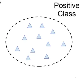
The second approach requires the estimation of the distribution followed by positive data. Thereby exam-ples that do not follow this distribution are regarded as negative. The need to assume a particular distribu-tion for the data limits these two approaches. The third approach looks for a boundary or frontier around pos-itive data, as shown in Fig.1. This border must accept as many objects belonging to the modeled class as pos-sible, while minimizing the acceptance of objects that do not belong to it [40].
Data outside the delimited boundary are consid-ered negative examples. Machine Learning (ML) tech-niques can be employed for defining these boundaries nonparametrically. Among the ML techniques adapted for this purpose, one frequently used is the Support Vector Machine (SVM) [34,40].
This paper employs a SVM version adapted to OCC, named ν-SVM [34], to evaluate the subsets of features selected. In ν-SVM, the data are first mapped into a space of higher dimension, where an hyperplane that separates positive data with maximal margin to the origin is found. Some training exam-ples are allowed to lay outside this region, in order to avoid overfitting to training data. The parameter ν ∈(0,1]limits the proportion of these examples. The hyperplane found corresponds to a non-linear fron-tier delimiting positive data in the original feature space. Mapping is performed by the employment of non-linear Kernel functions [8].
Fig. 1 Delimitation of positive data with circular boundary
3 Feature Selection
Feature Selection (FS) techniques look for a projec-tion of a dataset using a subset of the original input attributes. The selected features should be able to adequately represent the original examples from the modeled domain [23]. This dimensional reduction is possible due to the typical presence of irrelevant and redundant features in real datasets. Irrelevant features do not contribute to the distinction of the classes and can be directly eliminated. For redundant features, whose values are correlated, it is enough to keep just one representative of the related group.
FS can be formulated as a search for subsets of fea-tures that optimize some feature importance criterion [22]. It can be performed jointly to the classification model induction, in an embedded approach. The ML algorithm can also be employed as a black box to evaluate different subsets of features and guide the search throughout, in a wrapper approach. Finally, descriptors or measures extracted from data can be used to evaluate the importance of the features. In the later case we have a filter, which can be applied to any dataset despite of the classification technique used afterwards. This is the strategy employed by the technique presented in this paper.
The filter approach is generally faster when com-pared to embedded and wrapper approaches. In addi-tion, the preprocessed dataset can be used as input to any ML technique, since FS results are less biased towards a particular classification technique.
Various measures can be used to quantify the importance of the features for a classification prob-lem. According to Liu and Motoda [22], a feature is important if its removal leads to the deterioration of a given importance measure when compared to the value obtained while using that feature. These authors propose a taxonomy for the feature importance mea-sures, grouping them into the following categories [24]:
Consistency: tries to identify subsets of features that allow outputting a hypothesis consistent to the data. For labeled data, consistency is reflected by the presence of few similar examples with different labels in the dataset;
Dependency: also called measures of correlation or association, they quantify to which extent the value
of a feature can be predicted from the value of another feature. Thus, they verify how two features are associated with each other;
Distance: also known as measures of separability or discrimination, they consider as important those features that allow a better discrimination of the classes. Therefore, they reinforce that examples from different classes must be spatially distant; Information: considers the information gain
obtained when one or more features are used, com-pared to their removal. Generally some index based on the entropy or uncertainty arising from the use (or removal) of one or more features is used; Precision: takes into account the performance
achieved by a classifier when a given subset of fea-tures is selected. These measures are commonly adopted in wrapper FS.
We chose measures from all previous categories, except precision, to be combined in FS for OCC. This allows taking into account different aspects of the data for the FS. Precision measures were not considered because they are associated to wrapper FS.
Features can also be evaluated individually or jointly, in subsets. In the case each feature is evaluated isolatedly, a ranking of the features according to their importance regarding the measure adopted is output. Reduced subsets of features are obtained by select-ing the top-ranked features. When features are eval-uated jointly, usually some search procedure is also employed, which gradually adds or removes features from the subsets. In the experiments for this paper, we employed a set of measures for evaluating the features individually. Afterwards, their rankings are combined using different rank aggregation methods.
4 Feature Selection for OCC
There are not many studies investigating the use of FS in OCC. Most of the existing techniques are either based on wrapper [19] or use a dimensional reduction mechanism based on the aggregation of the feature values, like principal component analysis [18,21,44]. In [44] three filters for FS, usually adopted in data clustering, are employed in OCC tasks. The first, namedQ−α, is based on principles of group coher-ence [29].Q−αperforms FS while simultaneously grouping data. Therefore, it finds a subset of feaures
able to appropriately separate data into groups. Two other techniques are based on locality preservation, where the proximity in the original feature space must be preserved in the reduced feature subset. The first one is namedLocality Preserving Projections(LPP) [17], while the second one is theLaplacian score(LS) [16]. All techniques employed are suited for clustering problems and where used, without further adaptations, in the OCC context. TheQ−αtechnique obtained the best results in the experimental evaluations.
This paper extends [26] by including one more feature importance measure, by employing other aggregation strategy and improving the experiments. Section4.1presents the feature importance measures used in this work. Some of these measures were orig-inally designed for conventional classification prob-lems and had to be adapted to the peculiarities of the OCC scenario. Each of these measures produce a fea-ture ranking, where the feafea-ture at the top is considered to be more important for class discrimination.
Each measure provides a different perspective of the importance of the features. Therefore, we opted to combine their outputs in order to integrate multi-ple views of the data. We believe that this combination makes the FS technique more robust to eventual distor-tions or deficiencies of the individual measures when evaluating the selected feature set. Since each mea-sure produces a ranking of the features, we used three different rank aggregation methods for joining these feature rankings, which are described in Section4.2.
4.1 Feature Importance Measures
When measuring the importance of features in a clas-sification problem, the label of the examples is usually taken into account. For instance, the Correlation Based Filter (CBF) [14] employs an importance measure which considers a subset of features important if they are highly correlated to the class, while showing a low correlation to each other.
For OCC problems, all training examples have the same label. Therefore, an adaptation in the way the importance of the features is measured can be nec-essary. It is also possible to treat the problem as unlabeled and use FS techniques suited to unlabeled data [24]. However, adjustments may still be required, since in OCC problems it is important to choose features that enhance the characterization of only one-class, while in unsupervised learning one seeks for
subsets of features able to evidence multiple groups on data.
The following feature importance measures are adopted in this work:
Spectral score (SPEC): this measure allows the evaluation of features for both labeled and unla-beled datasets [47]. First a similarity matrixS for all pairs of data examples is built. The Radial Basis Function (RBF) can be used to compute the simi-larities, as shown in Equation1for two examples xi and xj. Based on this information, a graph G connecting the examples is obtained. The graphG hasnvertices, representingnobjects in the dataset, which are linked by connections weighted by the similarity between them. The concepts shown inS are reflected in the structure of G [7]. A feature consistent with the structure of the graph will have similar values for instances close to each other [47]. The spectrum ofGcan then be used to evaluate the features, ranking them according to their relevance. This criterion can also be used for datasets with a single class, allowing to rank the features according to their ability to maintain positive dataconsistent
andsimilar. Sij =e−
xi−xj2
2σ2 (1)
Information score(IS): the authors in [27] present aninformationmeasure for unlabeled data, shown in Equation2. The RBF similarity matrixSis used to calculate the entropy of the data, measuring its randomness. The entropy value is low when the similarity between the examples is high, favoring low intra-group randomness. This is an important issue for OCC too, where intra-class distances must be kept low. However, in its original version, this measure also attributes low entropy values to low similarity values. This occurs because, for cluster-ing purposes, high inter-groups distances must also be favored. This is not the case for OCC, where all data belong to the same class or, ultimately, to the same group. In this paper, we adapted this entropy measure to output low values only when the exam-ples are very similar and high values otherwise. For such, the similarities are normalized within the interval [0.5,1] instead of[0,1]. Thus, low simi-larities will be close to 0.5, which leads to a high entropy value. On the other hand, high similarities, next to 1, will lead to smaller entropy values, since
they indicate less randomness and a more structured dataset. To estimate the relevance of each feature according to this criterion, we measure the reduc-tion in the entropy advent from its eliminareduc-tion from the dataset. If the entropy decreases, the removal of the feature makes the data more homogeneous. In this case, the feature can be considered important. E= − n i=1 n j=1 Sijlog2Sij+(1−Sij)log2(1−Sij) (2) Pearson Correlation (PC): to quantify the asso-ciation of each feature with the others, we used the Pearson correlation measure. It allows checking whether the features are linearly related. Its val-ues are between -1 and 1. As both limits of the scale indicate high correlations, the absolute values of this measure were taken. Next, for each feature in the data, we measured its Pearson correlation to each of the other features and summed the absolute values calculated, as shown in Equation3. Features with high values for this index are very correlated to others. To favor the maintenance of features that represent more exclusive concepts, lower values are preferred. corr(fi)= m j=1 |pearson(fi, fj)| (3) Intra-class distance (ICD): given by Equation 4, wheren is the number of data instances and x¯ is the centroid of the class, this measure quantifies the distance from all examples of a class to the cen-troid of the class. Lower intra-class distances must be favored in OCC, in order to make positive data closer to each other. Like in IS, we measure the reduction in intra-class distance arising from the elimination of each individual feature. The features are then ranked such that those that approximate more the data are considered better. We employed the standard Euclidean distance measure in the computations. I E= 1 n n i=1 d (xi,x¯) (4)
Interquartile range (IQR): this measure takes into account the distribution of the feature values through their interquartiles. Its use is motivated by
the principle that if a feature is characteristic from a particular class, its values tend to be more concen-trated, which is reflected in the interquartile ranges. As an example, Fig.2shows box-plots of the fea-ture values in theirisdataset from the UCI repos-itory [2]. It is possible to notice that the classiris setosa, in the top, can be easily distinguished from the other classes by considering the values of the features petal length and petal width, which show more concentrated distributions. Although two fea-tures may have the same interquartile while their values overlap, this overlapping is more likely to occur if the values are widely dispersed.
Among the presented measures, only SPEC was employed without any adaptation. IS and ICD were adapted for OCC, while PC and IQR were proposed by the authors.
All measures allow to rank the features individ-ually. Nonetheless, each criterion gives a different emphasis to a particular aspect of the one-class dataset and has its deficiencies. For instance, IQR may attribute high rankings to features whose values may overlap to those from other classes. In fact, it is dif-ficult to take into account whether a feature is indeed discriminative when only information from a single class is available.
4.2 Rank Aggregation
The objective of rank aggregation is to combine the results produced by multiple rankings, generating a consensus ranking. In our case, as a result, a new order of importance for the features is produced. The pro-posed approach can also be regarded as a committee or ensemble of FS techniques [28,36,41,43,46].
Each importance measure produces a ranking of the features based on some data characteristic. For instance, the PC measure focus on poorly correlated features, while IQR ranks higher the features with more concentrated values. These criteria represent suboptimal evidence of the importance of the features and they have associated shortcomings. To incorporate the distinct aspects of the data considered by the dif-ferent importance measures, we decided to combine the rankings produced by them.
Combining multiple feature rankings also enables us to explore complementaries of the different measures and enhance FS by minimizing specific
influences of a single univariate measure in the results [45]. Thereby, multiple views of the importance of the features can be taken into account.
An important aspect to be considered is how to combine the rankings produced by the different mea-sures. There are different techniques proposed in the literature for ranking aggregation. The choice of a particular ranking technique can be based on the pre-dictive performance achieved when using the selected subset of features or on its computational cost.
One simple way to combine rankings is to average the positions of the features in the ranking lists [45]. Another alternative is to apply a majority voting rule for the positions attributed to each feature in the lists [3,42]. There are also methods to aggregate voting results from the areas of politics and social science [12]. This is the case of the Borda method [4], a posi-tional voting system proposed in 1784. In this method, each feature gets points according to its position in the rankings. These points increase from the first to the last place of a ranking. The feature with the smallest accumulated sum of points is ranked better.
Table 1presents the order of the features for the
iris-setosa class [2], obtained using the importance measures described in Section 4.1 and aggregating them according to the different rank aggregation meth-ods presented in this section. PL refers to the petal-lengthfeature, PW to thepetal-width feature, SL to
sepal-lengthand SW tosepal-width. We can observe how the rankings vary for different measures, since they consider distinct aspects of the data. For instance, for the SPEC importance measure, the following rank-ing of features is produced: SW, PW, PL and SL. After combining the different rankings of the features by the Mean (average) criterion, the result is: PW, PL, SL and SW. We deal with ties in the aggregation results by positioning the tied features according to their original ordering in the dataset.
Figure 3 represents the aggregation results from Table1graphically. The best (highest ranked) features are represented by darker shades of gray. Although there are some disagreements between ranking results, in general, we can observe that the features PL and PW assume higher positions.
There are many other rank aggregation methods in the literature and also empirical studies compar-ing some of them [3, 12, 41,45]. In general, there is no consensus on the best method to use. In [11], for example, the Mean is recommended, while in [31]
Fig. 2 Box-plotsof the feature values in theirisdataset. The top bars designate classIris-setosa, middle bars are from class Iris-versicolorand bottom bars are from classIris-virginica
a method named Schulze is considered better. In this study, three of the most common aggregation
meth-ods employed in the related literature, namely Mean, Majority and Borda, were investigated.
Table 1 Results of applying different feature aggregation measures foriris-setosaclass Features SL SW PL PW SPEC 4 1 3 2 Feature Inter-quartile 4 3 1 2 Importance Pearson 3 4 2 1 Measures Entropy 2 4 1 3 Intra-Class 1 4 3 2 Mean 3 4 2 1 Aggregation Majority 4 3 1 2 Methods Borda 4 1 3 2
Fig. 3 Aggregation results foriris-setosaclass
5 Experiments
This section presents the experiments performed in this work for the evaluation of the proposed FS tech-nique for OCC. All experiments were coded in Matlab using Weka [15] and LibSVM [5].
5.1 Datasets
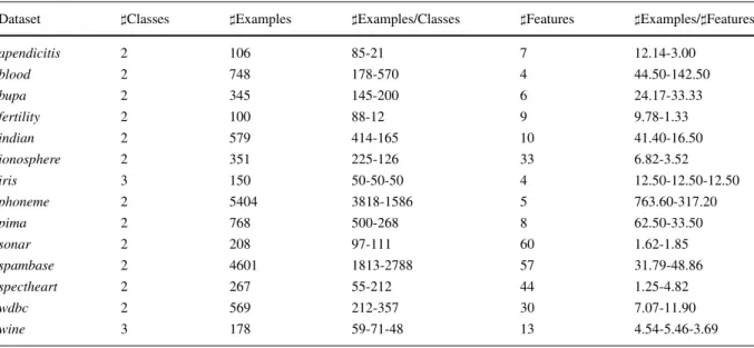
Fourteen datasets from the UCI [2] and Keel [1] repositories were used in the experiments. The main
characteristics of these datasets are illustrated in Table2, which presents, for each dataset: number of classes (Classes), number of examples (Examples), number of examples per class (Examples/Classes), number of features (Features) and number of exam-ples per feature (Examples/Features) for each class. For the later information, low ratios designate more sparse data. All features are continuous or integer val-ued, since some measures can only be calculated for numerical values. This does not prevent the use of nominal features, which have to be previously mapped into a numerical value.
One-class versions from these datasets were gener-ated by separating data from each of their classes. For instance, the blood dataset originates two one-class datasets: one for the classyesand another for the class
no. On the other hand, theirisdataset generates three one-class datasets: setosa, versicolor and virginica. The same reasoning applies to thewinedataset, giving rise to three class datasets, totalizing 30 one-class datasets for the experiments. This strategy is the same employed in related works regarding one-class datasets [39].
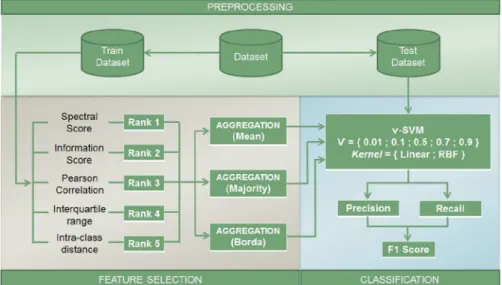
5.2 Methodology
Initially, all one-class datasets were divided according to the ten-fold cross-validation methodology. For each dataset, the training folds will have only the examples from one of the classes, 90 % of them. The test fold
Table 2 Summary of the characteristics of the datasets
Dataset Classes Examples Examples/Classes Features Examples/Features
apendicitis 2 106 85-21 7 12.14-3.00 blood 2 748 178-570 4 44.50-142.50 bupa 2 345 145-200 6 24.17-33.33 fertility 2 100 88-12 9 9.78-1.33 indian 2 579 414-165 10 41.40-16.50 ionosphere 2 351 225-126 33 6.82-3.52 iris 3 150 50-50-50 4 12.50-12.50-12.50 phoneme 2 5404 3818-1586 5 763.60-317.20 pima 2 768 500-268 8 62.50-33.50 sonar 2 208 97-111 60 1.62-1.85 spambase 2 4601 1813-2788 57 31.79-48.86 spectheart 2 267 55-212 44 1.25-4.82 wdbc 2 569 212-357 30 7.07-11.90 wine 3 178 59-71-48 13 4.54-5.46-3.69
has all the examples from the other classes, to simu-late the presence of negative data, plus 10 % of the examples from the training class.
For instance, in theiris-setosadataset, we will have ten test folds of size 105, where 5 examples are from the iris-setosa class and the remaining 100 exam-ples come from the other two classes (iris-virginica
andiris-versicolor). We highlight that all test data are not seen by any of the classification algorithms dur-ing induction nor by the feature selection techniques, which use only training data information.
The feature importance measures from Section4.1
are calculated for each training set partition. The fea-ture rankings produced are then aggregated using the Mean, Majority and Borda methods. We then system-atically remove the least important feature according to these methods from the training and test folds, until only the most important feature remains.ν-SVM clas-sifiers, with varyingνvalues and Kernel functions, are induced for the original datasets (with all features) and all of their reduced counterparts. The objective of this procedure is to monitor whether the number of fea-tures can be reduced while maintaining the predictive performance achieved when all features are used. The followingνvalues were tested: 0.01, 0.1, 0.5, 0.7 and 0.9. The Kernel functions tested were the RBF and the Linear, with the default parameters from the LibSVM tool [6]. This totalizes 10 combinations of parameter values for theν-SVM classifiers.
The F1 measure was used to evaluate the predic-tive performance of the classifiers for the different experimental setups investigated in this study (5). It measures the ability to correctly retrieve the positive data by combining the precision (P, defined by Equa-tion6) and recall (R, defined by Equation7) obtained for the positive class.
F1=2(P∗R) (P+R) (5) P = T P T P +F P (6) R= T P T P +F N (7)
In the Equations6and7, TP refers to the number of true positive examples in test data, FP is the number of false positive examples and FN stands for the num-ber of false negative examples. Therefore, while the precision measures whether the examples predicted
as positive are indeed positive, recall represents the positive data fraction that was correctly retrieved.
The overall methodology employed is outlined in Fig. 4. For each training partition i of a one-class dataset, we apply the five feature importance mea-sures, aggregate their results and induce ν-SVMs using decreasing numbers of features. The F1 perfor-mance achieved on the test fold i is then recorded. Since all datasets were divided with ten-fold cross-validation, average and standard-deviation of the F1 results are calculated.
6 Experimental Results
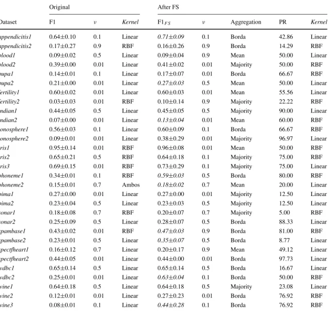
Several experiments were performed to evaluate FS for OCC using the previously mentioned datasets. Table 3presents the best F1 results obtained in the experiments for each one-class dataset. It shows the F1 average performance and standard deviation, obtained by following the cross-validation methodology, for both original data (with all features) and the data obtained after FS (using the format average F1 ± standard-deviation). The FS results correspond to the best configuration among all tested combinations of aggregation methods and ν-SVM parameter values. Table3also shows theν values and Kernel function associated with the reported results. For the results after FS, we also present the rank aggregation method employed and the percentage of reduction (PR) in the number of features after FS. The best F1 in each dataset is highlighted in boldface. When the results after FS are significantly different from those obtained for the original data, they are highlighted in bold-face and italics. The statistical test employed was the paired Wilcoxon signed-ranks test [9], with 95 % of confidence level.
Next we discuss the results concerning: the F1 values obtained; the reduction in the number of fea-tures; the aggregation strategies employed; theν-SVM parameter values; the precision and recall of the clas-sifiers; and a trade-off between the F1 values achieved and the percentage of reduction in the number of features.
6.1 F1 Measure Values
It is possible to notice in Table3that the use of FS either maintained or improved the F1 rates for most of
Fig. 4 Methodology employed in the experiments for each data fold
the datasets. Employing the paired Wilcoxon signed-ranks statistical test [9] with a 95 % of confidence value, it is possible to observe that:
1. The F1 performance was significantly improved after FS for the datasets: appendicitis1, bupa2,
indian2, phoneme1, phoneme2, spambase1,
spambase2,wdbc2andwine3.
2. For all other datasets, the F1 performance was maintained after FS, when compared to the origi-nal F1 values.
Therefore, FS was always capable to either maitain (in 21 datasets) or significantly improve (in nine datasets) the predictive performance of the one-class classifiers, while using less predictive features. It is interesting to notice that some of the major per-formance gains occurred for some of the datasets with more features, likephoneme1,phoneme2, spam-base1, spambase2 and wdbc2. Overall, there were more predictive performance gains for datasets with more examples. Since we adopt a filter approach, which consider aspects from data, this is a somewhat expected result.
Taking each dataset paired according to its orig-inal domain, some interesting results can be seen. For example, class appendicitis1 was more accu-rately identified than class appendicitis2, according to the F1 measure. The same happens for the pairs
blood1-blood2, fertility1-fertility2, indian1-indian2,
phoneme1-phoneme2andspectheart1-spectheart2. In all these pairs, the class with lowest predictive
performance is the one with the smallest number of examples.
6.2 Reduction in the Number of Features
The reductions in the number of features were mostly large. There are several cases (19 out of 30 datasets) where the reduction in the number of features was higher than or equal to 50 %, which can be consid-ered a sharp decrease. Smaller reductions occurred in the datasetssonar1andspambase2. In absolute num-bers, three features were removed from the sonar1
dataset, while five features were removed from the
spambase2dataset. As these datasets have a high num-ber of features, their percentage of feature reduction was low.
Finally, reductions of 90 % or more in the num-ber of features were obtained for the indian1, iono-sphere2 and spectheart2 datasets. The ionosphere2
and spectheart2 datasets, particularly, are originally sparse datasets, which may have benefited more from the dimensional reduction promoted by FS.
6.3 Aggregation Strategies
The results obtained by the three aggregation strate-gies employed were similar, although the Borda method had the best predictive performance in a larger number of datasets. While Borda was the best in 14 cases, Majority figured as the best in 9 datasets and Mean outperformed Borda and Majority in 7 of
Table 3 Best results achieved for original data and for the feature selectors
Original After FS
Dataset F1 ν Kernel F1F S ν Aggregation PR Kernel
appendicitis1 0.64±0.10 0.1 Linear 0.71±0.09 0.1 Borda 42.86 Linear
appendicitis2 0.17±0.27 0.9 RBF 0.16±0.26 0.9 Borda 14.29 RBF
blood1 0.09±0.02 0.5 Linear 0.09±0.04 0.9 Mean 50.00 Linear
blood2 0.39±0.00 0.01 Linear 0.41±0.02 0.01 Majority 50.00 RBF
bupa1 0.14±0.01 0.1 Linear 0.17±0.07 0.01 Borda 66.67 RBF
bupa2 0.21±0.00 0.01 Linear 0.27±0.03 0.5 Mean 50.00 Linear
fertility1 0.60±0.02 0.01 Linear 0.60±0.03 0.01 Mean 55.56 Linear
fertility2 0.03±0.03 0.01 RBF 0.10±0.14 0.9 Majority 22.22 RBF
indian1 0.44±0.05 0.5 Linear 0.45±0.05 0.5 Majority 90.00 Linear
indian2 0.07±0.00 0.01 Linear 0.13±0.04 0.01 Mean 60.00 RBF
ionosphere1 0.56±0.03 0.1 Linear 0.60±0.09 0.1 Borda 66.67 RBF
ionosphere2 0.09±0.01 0.01 Linear 0.38±0.29 0.01 Majority 96.97 Linear
iris1 0.95±0.14 0.01 RBF 0.96±0.08 0.01 Mean 50.00 RBF
iris2 0.65±0.21 0.5 RBF 0.64±0.18 0.1 Majority 75.00 RBF
iris3 0.69±0.15 0.01 RBF 0.73±0.29 0.1 Majority 75.00 Linear
phoneme1 0.34±0.01 0.1 RBF 0.59±0.03 0.5 Borda 80.00 RBF
phoneme2 0.15±0.01 0.7 Ambos 0.18±0.02 0.7 Mean 20.00 Linear
pima1 0.27±0.00 0.01 Linear 0.27±0.00 0.01 Majority 12.50 Linear
pima2 0.23±0.04 0.5 Linear 0.23±0.03 0.5 Majority 12.50 Linear
sonar1 0.18±0.08 0.7 RBF 0.20±0.07 0.7 Majority 5.00 RBF
sonar2 0.25±0.09 0.5 Linear 0.28±0.07 0.5 Borda 88.33 Linear
spambase1 0.43±0.02 0.01 RBF 0.47±0.03 0.9 Borda 81.00 RBF
spambase2 0.23±0.01 0.5 Linear 0.35±0.07 0.5 Borda 8.77 Linear
spectfheart1 0.16±0.12 0.7 Linear 0.20±0.17 0.9 Mean 49.12 Linear
spectfheart2 0.44±0.05 0.01 Linear 0.44±0.00 0.01 Borda 97.73 Linear
wdbc1 0.65±0.14 0.5 Linear 0.65±0.14 0.5 Borda 16.67 Linear
wdbc2 0.25±0.01 0.01 Linear 0.63±0.04 0.1 Borda 50.00 RBF
wine1 0.64±0.18 0.5 Linear 0.64±0.18 0.5 Majority 23.08 Linear
wine2 0.12±0.01 0.01 Linear 0.27±0.23 0.01 Borda 76.92 RBF
wine3 0.08±0.01 0.1 Linear 0.44±0.28 0.1 Borda 76.92 RBF
the datasets. The Borda aggregation method is some-what costly, and this can be taken into account when choosing a particular aggregation method. Mean and Majority are computed in O(n) while BordaO(n2). Nonetheless, it is advisable to test all strategies exper-imentally before choosing an aggregation method for a given dataset.
The percentage of reduction (PR) in the num-ber of features obtained by the aggregation strategies were: 55.76±28.72 for Borda; 46.23±35.35 for Majority; and 54.05±21.31 for Mean. Therefore,
similar PR values were also obtained by the aggrega-tion strategies.
6.4 SVM Parameter Values
Concerning theν-SVM parameter values, it is possi-ble to notice in Tapossi-ble3that theLinearKernel excelled for the original datasets. However, after FS, there were cases where a non-linear boundary became necessary and theRBFKernel showed better results. Theν val-ues remained similar in most of the cases, increasing
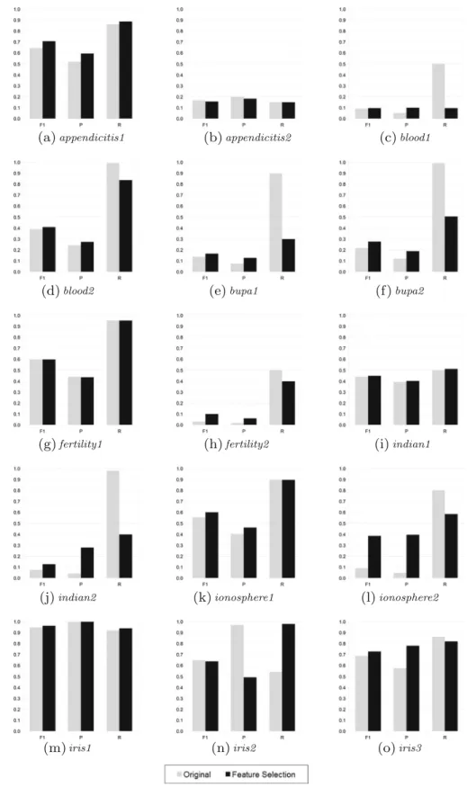
Fig. 5 Plots of the F1, precision and recall values per dataset - part 1. Gray columns correspond to original results, while black columns show results after FS
Fig. 6 Plots of the F1, precision and recall values per dataset - part 2. Gray columns correspond to original results, while black columns show results after FS
in several others. This implies in the need for fron-tiers less restricted to the positive training data after the application of FS.
6.5 Precision and Recall
For better assessing whether the F1 variations are due to changes in precision or recall, in the Figs.5and6
we present plots of the F1, precision and recall aver-age values achieved for each dataset. Two columns are drawn per performance metric, one for the results in the original data (light gray), and the other for the results achieved after the FS procedure (black).
It is possible to notice from these figures that, after the FS, an increase in the precision values often occurs. Precision accounts for the correct positive predictions, i.e., it is larger when more data pre-dicted as positive are indeed from the target class. This result is interesting, since the false positive rate cannot be directly minimized when training one-class one-classifiers, because counterexamples are absent at this stage. FS seems to have minimized this effect.
There were cases where the increase in precision was obtained at the cost of a reduction in recall, namely the occurrence of more false negatives. There is usually a trade-off between precision and recall rates, so that if one increases the other decreases. But there are also cases where both precision and recall values increased after the FS. This is the case, for example, of the datasets appendicitis1, indian1
andsonar2, which showed room for improvement in the predictions for both positive and negative classes, which was exploited by the FS.
6.6 Trade-off F1 Versus PR
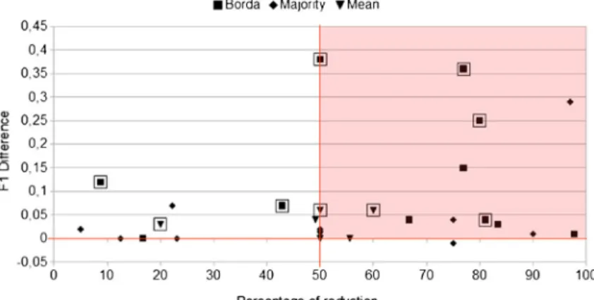
Figure 7 presents an overview of the FS results for all datasets, associating the percentage of reduction in the number of features (x axis) with the difference between the F1 value before and after the FS (y axis). The closer the point is to the extreme right of the graph, the better is the corresponding result, since it represents higher gains in F1 while using less features. The region representing gains in F1 and large reduc-tions in the number of features (higher or equal to 50 %) is shaded. Datasets for which the F1 gains were statistically significant are highlighted with a square. It is worth noting that many of the statistically signif-icant predictive results were obtained using less than 50 % of the original features.
It is possible to observe, in many cases, improve-ments of predictive results with large reductions in the number of features. In several datasets the reductions in the number of features was higher than 50 %, a significative dimensional reduction. The Borda aggre-gation method showed more F1 gains and larger reductions in the number of features, when compared to the other aggregation methods.
Overall, we should also observe that many of the single class results observed in this work can be con-sidered poor if compared with the performance that can be obtained when treating the same data by stan-dard binary or multi-class techniques. This may be due to the inherent difficulty of OCC when compared to standard classification scenarios, but also to the fact that the datasets used are not naturally one-class. Future work shall investigate the performance of the proposed FS technique for real one-class applications.
Fig. 7 Feature reduction percentage versus F1 gains after the FS
7 Conclusion
This paper presented a new filter approach for fea-ture selection in one-class classification problems. The proposed method combines rankings of the fea-tures selected by different feature importance mea-sures. The chosen measures are able to capture distinct aspects from the data. Thereby, their combination allow exploring multiple and complementary views of the data.
Each importance measure combined belongs to one or more categories among those listed in [24]: the spectral score measures the consistency relative to data structure; the information score calculation has been adapted to the one-class context in this work and focuses on features that bring a higher informa-tiongain for the target class; the correlation between the features considers theassociation between them, allowing the removal of redundant features; the intra-classdistancefocuses on preserving the locality of the data from the target class; and the inter-quartile range, introduced in this paper, is based on thedistributionof the features in the target class. Each of these measures provides evidence of the importance of the features that can be complemented by their combination. To combine their results, three different ranking aggre-gation strategies were employed: Mean, Majority and Borda.
Experiments were performed on 30 artificial one-class datasets generated from binary and multione-class datasets obtained from public repositories. It was pos-sible to reduce data dimension while maintaining or event improving one-class classification predictive performance, especially regarding the precision in the recognition of the target class. We thereby proved the hypothesis of the work that it is possible to perform FS in OCC tasks using only descriptors extracted from the target class data.
It is worth mentioning that, in many cases, the use of FS also reduced the number of false positives. As the false positive rate cannot be minimized directly during the induction of one-class classifiers, this result is important and reinforces that this deficiency can be reduced if data are properly preprocessed.
As future work, we plan to employ the inves-tigated technique in one-class real applications and datasets. Other one-class classification techniques can also be employed for evaluating the subsets of features selected, since, in the filter approach, the results are
independent of the classification technique employed. This can also provide the achievement of more gen-eral experimental results. It would also be interest-ing to investigate and highlight which are the char-acteristics of the datasets for which FS was more beneficial.
Acknowledgments The authors would like to thank the Coordenac¸˜ao de Aperfeic¸oamento de Pessoal de N´ıvel Supe-rior (CAPES), the Conselho Nacional de Desenvolvimento Cient´ıfico e Tecnol´ogico (CNPq) and the Fundac¸˜ao de Amparo `a Pesquisa do Estado de S˜ao Paulo (FAPESP) for their financial support.
References
1. Alcal ˜A-Fdez, J., Fernandez, A., Luengo, J., Derrac, J., Garca, S., Snchez, L., Herrera, F.: Keel data-mining soft-ware tool: Data set repository, integration of algorithms and experimental analysis framework. J. Multiple-Valued Logic Soft Comput.17(2-3), 255–287 (2011)
2. Bache, K., Lichman, M.: UCI machine learning repository (2014).http://archive.ics.uci.edu/ml
3. Bauer, E., Kohavi, R.: An empirical comparison of voting classification algorithms: Bagging, boosting, and variants. Mach. learn.36(1-2), 105–139 (1999)
4. De Borda, J.C.: M˙emoire sur les ˙elections au scrutin. Histoire de l’Acad˙emie Royale des Sciences (1784) 5. Chang, C.C., Lin, C.J.: Libsvm: a library for support
vec-tor machines. ACM Trans. Intell. Syst. Technol.2(3), 1–30 (2011)
6. Chang, C.C., Lin, C.J.: Libsvm: a library for support vec-tor machines. ACM Trans. Intell. Syst. Technol.2(3), 1–30 (2011)
7. Chapelle, O., Scholkopf, B., Zien, A.: Semi-supervised Learning, Chap. Graph-Based Methods. The MIT Press (2006)
8. Cristianini, N., Shawe-Taylor, J.: An Introduction to Sup-port Vector Machines and other kernel-based learning methods. Cambridge University Press (2000)
9. Dem˙sar, J.: Statistical comparisons of classifiers over mul-tiple data sets. J. Mach. Learn. Res.7, 1–30 (2006) 10. Deris, S., Alashwal, H., Othman, M.: One-class
sup-port vector machines for protein-protein interac-tions prediction. Int. J. Biol. Med. Sci. 1(2), 120–127 (2006)
11. Dittman, D.J., Khoshgoftaar, T.M., Wald, R., Napolitano, A.: Classification performance of rank aggregation tech-niques for ensemble gene selection. In: The Twenty-Sixth International FLAIRS Conference (2013)
12. Dwork, C., Kumar, R., Naor, M., Sivakumar, D.: Rank aggregation methods for the web. In: Proceedings of the 10th international conference on World Wide Web, pp. 613–622. ACM (2001)
13. Elith*, J., H. Graham*, C., P. Anderson, R., Dud?k, M., Fer-rier, S., Guisan, A., J. Hijmans, R., Huettmann, F., R. Leath-wick, J., Lehmann, A., Li, J., G. Lohmann, L., A. Loiselle,
B., Manion, G., Moritz, C., Nakamura, M., Nakazawa, Y., McC. M. Overton, J., Townsend Peterson, A., J. Phillips, S., Richardson, K., Scachetti-Pereira, R., E. Schapire, R., Sober?n, J., Williams, S., S. Wisz, M., E. Zimmermann, N.: Novel methods improve prediction of species? distributions from occurrence data. Ecography29(2), 129–151 (2006). doi:10.1111/j.2006.0906-7590.04596.x
14. Hall, M.: Correlation-based feature selection for discrete and numeric class machine learning. In: Proceedings 17th International Conference Machine Learning, pp. 359–366 (2000)
15. Hall, M., Frank, E., Holmes, G., Pfahringer, B., Reute-mann, P., Witten, I.H.: The weka data mining software: an update. SIGKDD Explor. Newsl.11(1), 10–18 (2009). doi:10.1145/1656274.1656278
16. He, X., Cai, D., Niyogi, P.: Laplacian score for feature selection. In: NIPS, Vol. 186, p. 189 (2005)
17. He, X., Niyogi, P.: Locality preserving projections. In: NIPS, Vol. 16, pp. 234–241 (2003)
18. Hoffmann, H.: Kernel pca for novelty detection. Patt. Recogn.40(3), 863–874 (2007)
19. Jeong, Y.S., Kang, I.H., Jeong, M.K., Kong, D.: A new fea-ture selection method for one-class classification problems. Systems, Man, and Cybernetics, Part C: Applications and Reviews. IEEE Trans.42(6), 1500–1509 (2012)
20. Khan, S.S., Madden, M.G.: A survey of recent trends in one class classification. Artif. Intell. Cogn. Sci.6206, 188–197 (2010)
21. Lian, H.: On feature selection with principal component analysis for one-class svm. Pattern Recogn. Lett.33(9), 1027–1031 (2012)
22. Liu, H., Motoda, H.: Feature Extraction, Construction and Selection - A Data Mining Perspective. Kluwer Academic Publishers (1998)
23. Liu, H., Motoda, H., Setiono, R., Zhao, Z.: Feature selection : An ever evolving frontier in data mining. Knowl. Creat. Diffus. Utilization4, 4–13 (2010)
24. Liu, H., Yu, L.: Toward integrating feature selection algo-rithms for classification and clustering. IEEE Trans. Knowl. Data Eng.17(4), 491–502 (2005)
25. Lorena, A.C., Jacintho, L.F.O., Siqueira, M.F., Giovanni, R., Lohmann, L.G., Carvalho, A.C.P.L.F., Yamamoto, M.: Comparing machine learning classifiers in potential dis-tribution modelling. Expert Syst. Appl. 38, 5268–5275 (2011)
26. Lorena, L.H.N., De Carvalho, A.C.P.L.F., Lorena, A.C.: Seleo de atributos em problemas de classificao com uma nica classe [in portuguese]. In: X Encontro Nacional de Inteligncia Artificial e Computacional (ENIAC), pp. 1–11 (2013)
27. Mitra, P., Murthy, C.A., Pal, S.: Unsupervised feature selec-tion using feature similarity. IEEE Trans. Pattern Anal. Mach. Intell.24(3), 301–312 (2002)
28. Namsrai, E., Munkhdalai, T., Li, M., Shin, J.H., Namsrai, O.E., Ryu, K.H.: A feature selection-based ensemble method for arrhythmia classification. JIPS 9(1), 31–40 (2013)
29. Ng, A.Y., Jordan, M.I., Weiss, Y.: On spectral clustering analysis and an algorithm. Proceedings of Advances in Neural Information Processing Systems. Cambridge, MA: MIT Press14, 849–856 (2001)
30. Pimentel, M.A., Clifton, D.A., Clifton, L., Tarassenko, L.: A review of novelty detection. Sig. Process.99(0), 215–249 (2014)
31. Prati, R.C.: Combining feature ranking algorithms through rank aggregation. In: Neural Networks (IJCNN), The 2012 International Joint Conference on, pp. 1–8. IEEE (2012)
32. Reyes, J., Gilbert, D.: Combining one-class classifica-tion models based on diverse biological data for predic-tion of protein-protein interacpredic-tions. In: Data Integrapredic-tion in the Life Sciences, Lecture Notes in Computer Sci-ence, Vol. 5109, pp. 177–191. Springer Berlin Heidelberg (2008)
33. Reyes, J.A., Gilbert, D.: Prediction of protein-protein inter-actions using one-class classification methods and integrat-ing diverse data. J. Integr. Bioinforma.4(3), 77 (2007) 34. Scholkopf, B., Plattz, J.C., Shawe-Taylory, J., Smolax,
A.J., Williamson, R.C.: Estimating the support of a high-dimensional distribution. Neural Comput. 13(7), 1443– 1471 (2001)
35. Shahid, N., Aleem, S., Naqvi, I.H., Zaffar, N.: Support vec-tor machine based fault detection & classification in smart grids. In: Globecom Workshops (GC Wkshps), 2012 IEEE, pp. 1526–1531. IEEE (2012)
36. Shen, Q., Diao, R., Su, P.: Feature selection ensemble. In: A. Voronkov (ed.) Turing-100, EPiC Series, Vol. 10, pp. 289–306. EasyChair (2012)
37. Shin, H.J., Eom, D.H., Kim, S.S.: One-class support vec-tor machines-an application in machine fault detection and classification. Comput. Ind. Eng.48(2), 395–408 (2005). doi:10.1016/j.cie.2005.01.009
38. Smart, E., Brown, D.J., Axel-Berg, L.: Comparing one and two class classification methods for multiple fault detection on an induction motor. In: ISIEA, 2013 IEEE Symposium on (2013)
39. Tax, D.M., Duin, R.P.: Characterizing one-class datasets. In: Proceedings of the Sixteenth Annual Symposium of the Pattern Recognition Association of South Africa, pp. 21–26 (2005)
40. Tax, D.M.J.: One-class classification: Concept-learning in the absence of counter-examples. PhD dissertation, Delft University of Technology (2001)
41. Tsymbal, A., Cunningham, P.: Diversity in ensemble fea-ture selection. Tech. rep., Department of Computer Science, Trinity College Dublin (2003). URLhttp://www.cs.tcd.ie/ publications/tech-reports/reports.03/TCD-CS-2003-44.pdf
42. Tsymbal, A., Pechenizkiy, M., Cunningham, P.: Diversity in search strategies for ensemble feature selection. Inf. fusion
6(1), 83–98 (2005)
43. Tsymbal, A., Puuronen, S., Patterson, D.W.: Ensemble feature selection with the simple bayesian classification. Information Fusion4(2), 87–100 (2003)
44. Villalba, S.D., Cunningham, P.: An evaluation of dimen-sion reduction techniques for one-class classification. Artif. Intell. Rev.27(4), 273–294 (2007)
45. Wald, R., Khoshgoftaar, T.M., Dittman, D., Awada, W., Napolitano, A.: An extensive comparison of feature ranking aggregation techniques in bioinformatics. In: Information Reuse and Integration (IRI), 2012 IEEE 13th International Conference on, pp. 377–384. IEEE (2012)
46. Zhang, D., Wang, Y.: A new ensemble feature selection and its application to pattern classification. J. Control Theory Appl.7(4), 419–426 (2009)
47. Zhao, Z., Liu, H.: Spectral feature selection for supervised and unsupervised learning. In: Proceedings 24th Interna-tional Conference on Machine Learning, pp. 1151–1157 (2007)