MsRi-CCF: Multi-Scale and Rotation-Insensitive Convolutional Channel Features for Geospatial Object Detection

remote sensing

MsRi-CCF: Multi-Scale and Rotation-Insensitive

Convolutional Channel Features for Geospatial

Object Detection

Xin Wu1,2,†, Danfeng Hong3,4,† , Pedram Ghamisi5 , Wei Li1,2and Ran Tao1,2,*

1 _{School of Information and Electronics, Beijing Institute of Technology (BIT), Beijing 100081, China;}

[email protected] (X.W.); [email protected] (W.L.)

2 _{Beijing Key Laboratory of Fractional Signals and Systems, School of Information and Electronics,}

Beijing Institute of Technology (BIT), Beijing 100081, China

3 _{Remote Sensing Technology Institute (IMF), German Aerospace Center (DLR), 82234 Wessling, Germany;}

[email protected]

4 _{Signal Processing in Earth Observation (SiPEO), Technical University of Munich (TUM),}

80333 Munich, Germany

5 _{Machine Learning Group, Exploration Division, Helmholtz Institute Freiberg for Resource Technology,}

Helmholtz-Zentrum Dresden-Rossendorf, 09599 Freiberg, Germany; [email protected] * Correspondence: [email protected]

† These authors contributed equally to this work.

Received: 5 November 2018; Accepted: 6 December 2018; Published: 8 December 2018 Abstract:Geospatial object detection is a fundamental but challenging problem in the remote sensing community. Although deep learning has shown its power in extracting discriminative features, there is still room for improvement in its detection performance, particularly for objects with large ranges of variations in scale and direction. To this end, a novel approach, entitled multi-scale and rotation-insensitive convolutional channel features (MsRi-CCF), is proposed for geospatial object detection by integrating robust low-level feature generation, classifier generation with outlier removal, and detection with a power law. The low-level feature generation step consists of rotation-insensitive and multi-scale convolutional channel features, which were obtained by learning a regularized convolutional neural network (CNN) and integrating multi-scaled convolutional feature maps, followed by the fine-tuning of high-level connections in the CNN, respectively. Then, these generated features were fed into AdaBoost (chosen due to its lower computation and storage costs) with outlier removal to construct an object detection framework that facilitates robust classifier training. In the test phase, we adopted a log-space sampling approach instead of fine-scale sampling by using the fast feature pyramid strategy based on a computable power law. Extensive experimental results demonstrate that compared with several state-of-the-art baselines, the proposed MsRi-CCF approach yields better detection results, with 90.19% precision with the satellite dataset and 81.44% average precision with the NWPU VHR-10 datasets. Importantly, MsRi-CCF incurs no additional computational cost, which is only 0.92 s and 0.7 s per test image on the two datasets. Furthermore, we determined that most previous methods fail to gain an acceptable detection performance, particularly when they face several obstacles, such as deformations in objects (e.g., rotation, illumination, and scaling). Yet, these factors are effectively addressed by MsRi-CCF, yielding a robust geospatial object detection method.

Keywords:AdaBoost; deep learning; object detection; optical remote sensing imagery; outlier removal; multi-scale aggregation; rotation-insensitive

1. Introduction

In recent years, the successful launch of optical broadband (multispectral) and very high resolution (VHR) RGB satellites has made the spaceborne remote sensing images available on a large and even global scale. This has attracted increasing interest in the analysis and interpretation of optical remote

sensing images (RSIs), including activities such as classification and recognition [1–3], object detection

and tracking [4,5], and spectral unmixing [6,7]. In particular, geospatial object detection [8–12] has

gained considerable attention, owing to the great applications to hazard response, urban monitoring,

and management. In [8], Cheng et al. roughly categorized the geospatial object detection approaches

into template matching-, knowledge-, object-, and learning-based methods. Notably, the objects in remote sensing datasets inevitably suffer from complex image deformations (e.g., multi-resolution, illumination, direction variation, occlusion, etc.). By ignoring the embedding of local and global information, these methods fail to obtain highly distinguishable semantic information. This can lead to a major challenge for extracting discriminative and generalized features.

With a powerful learning ability, deep learning-based techniques [13–15] have been widely

applied to geospatial object detection. Deep neural networks (DNN) have been proven to be effective

for extracting hierarchical feature representation (from low-level to high-level) [16–18]. Nevertheless,

the limited receptive fields to multi-resolution images and the sensitivity to rotation behaviors prevent

these networks from performing better [19–22]. Therefore, the elaborate design of robust features

with regard to scaling and rotation plays a critical role in the detection task. Recently, some advanced

methods [19,23–25] have been accordingly proposed, but their solutions may be effective only for

an individual issue mentioned above. For instance, a deep adaptive proposal network [19] was

established by jointly considering low-level and high-level outputs to enhance feature representation.

Cheng et al. [23] learned a new rotation-invariant layer on the basis of existing convolutional neural

network (CNN) architectures with a new loss function. Chen et al. [24,25] presented a hybrid CNN to

extract multi-scale features for vehicle detection through satellite images. To date, CNN (or perhaps

DNN in general) continues to deepen, increasing from the 8 layers of AlexNet [26] to the 152 layers of

ResNets [27] within 3 years. Although these state-of-the-art deep networks have achieved competitive

detection results by utilizing a variety of feature maps from the original input to the output of the soft-max layer, their concepts are dramatically affected by additional time and space costs. Therefore, it is important to develop a relatively light-weighted network architecture with scale and direction robustness in the case of geospatial object detection.

AdaBoost [28,29], a typical boosting algorithm, iteratively selects weak classifiers (e.g., binary decision

trees) from a pool of candidates and targets the hard examples from the previous round. Compared with the end-to-end CNN method, it has lower computation and storage costs. In this study, we designed an object detection framework with low-level multi-scale and direction-insensitive feature representations for optical RSIs to address the tedious fine-tuning of high-level connections in CNN during the adaptation of various classification/regression problems. To the best of our knowledge, this is the first work of this kind

to combine the convolutional channel feature (CCF) [30] with AdaBoost and a CNN for applications to

various detection tasks (e.g., pedestrian, face, edge detection, etc.). There are other extended algorithms

based on using CNNs as weak classifiers [31] or weighting the input samples in order to optimally perform

CNN learning [32]. However, object detection based on these methods is basically conducted on street

view images, and the use of remote sensing imagery is less investigated. Therefore, such approaches usually fail to work well when applied to geospatial object detection because of the complex nature of geospatial data, including variations in scaling and direction.

To this end, we propose a novel geospatial object detection framework by usingmulti-scale and

rotation-insensitiveconvolutionalchannelfeatures (MsRi-CCF), as illustrated in Figure1. Diverging

from the CCF, we started with rotation-insensitive feature learning to alleviate the performance degradation due to large-scale object rotation. To locate and recognize differently sized objects more effectively, we then modeled the multi-scale feature representation by integrating multi-resolution convolutional maps. Prior to feeding these features into the AdaBoost classifier, the outlier removal

method was used to screen out the high-quality samples for training. Such a strategy can effectively correct the bias and variance of the trained classifier caused by the outliers, yielding a more robust detector. In the test phase, a fast feature pyramid was embedded to achieve fast yet approximately lossless finely sampled feature extraction. More specifically, the main highlights of our work can be summarized as follows:

• Proposal of a geospatial object detection framework by jointly investigating robust low-level

feature generation, classifier generation with outlier removal, and detection with a power law which can simultaneously block large ranges of scale, directional variation, and interference of pseudo-label samples;

• Generation of robust low-level feature maps which are based on adding two modules to the

original CNN, namely, the rotation-insensitive descriptor and multi-scale convolutional channel feature. We implemented these modules by adding the regularization constraint to the objective function of the network model. These features were generated in an extended and complementary way to ensure the integrity of the information.

• In order to suppress the influence of outliers on its exponential loss function, the Gamma Mixture

Model (GaMM) outlier removal method is introduced to minimize the classification error caused by pseudo-label samples, among other factors.

Figure 1.The architecture of the proposed multi-scale and rotation-insensitive convolutional channel features (MsRi-CCF) method. The feature generation step in the training phase is detailed in Figures2and3. These generated features are then fed into the AdaBoost classifier with outlier removal (see Figure4for more details) for the final classification and localization. In the test phase, a fast feature pyramid is applied for the final predictions.

The remainder of this paper is organized as follows. In Section2, we introduce the proposed

MsRi-CCF framework. Experimental results on a satellite dataset and NWPU VHR-10 are presented in

2. Methodology

The novel MsRi-CCF object detection framework for optical RSIs consists of three phases, including robust low-level (shallow) feature generation, classifier generation with outlier removal, and detection with a power law. The architecture of the proposed MsRi-CCF framework is illustrated

in Figure1. In the proposed method, due to the limited size of the training sets, we rotated, flipped,

rescaled, and processed the hue and saturation in advance, and we then fed them to the revised CNN

for automatic feature learning. The specific workflow is summarized inAlgorithm1.

Algorithm 1MsRi-CCF Detector

Input:The set of training samples for the current class,D= (x1,y1),(x2,y2),· · ·,(xN,yN);

yi =1 indicates positive samples;yi=0 indicates negative samples; the number of

current classes,N; additional rotating training samples,Dϕ=

Dϕ1,Dϕ2,· · ·,DϕK ,

and initialized AdaBoost,det0;

Output:AdaBoost classifiers, weight of the current iteration,detiandωi 1 InitializeLoad pretrained VGG-16 parameters,Pre_param;

2 expanded data after preprocessing (see Section3.2),D,D_ϕ ;

3 feature_maps = FeatureExtraction(D,D_ϕ ,Pre_param);

4 whilenot end of convergencedo 5 fort=1,· · ·,Tdo

6 Initializeωrandomly weight normalization,qt,i = ωt,i

∑(j=1N+K+L)ωt,j

;

7 select the best weak classifier with the minimum error rateεtusing Equation (4);ht(x);

8 updateβt= ₁₋εt_ε t; 9 ωt+1,i =ωt,iβ1_t−ei,ei={0, 1}; 10 αt=log1_β; 11 if∑T_t=1αtht(x)≥ 1₂∑Tt=1αtthen 12 replaceB_iwithB_i−1;

13 return classifiersdet_i,ωi;

14 compute direction-based regularization constraint term using Equation (1);

15 compute objective functionJ(θ,ϕ,netWI,BI)using Equation (3);

16 updatenetwaandba.

For robust low-level feature generation, two submodules, namely, the rotation-insensitive descriptor and multi-scale aggregated descriptor, were designed and linked to the original VGG-16 network (To maintain consistency and comparability, we started with the same VGG-16 architecture for the CCF as the feature extractor. Furthermore, we aimed to improve the robustness to scaling and rotation rather than aggressively pursuing performance gain. The ResNet is proven to be effective for reducing the training error of very deep networks. For not-so-deep networks, plain networks and ResNet should not largely differ. As a trade-off, the VGG-16 network was applied in our case.) to avoid direction variation and a large scale range, which are usually caused by different shapes

and structures. The detailed framework of the module, illustrated in Figures2and3, allows for

increasing the step size of the direction rotation and the depth of the network to a certain extent, thereby improving the distinguishability of the features and the generalization performance of the

framework. In detail, the regularized constraint term, inspired by Reference [23], was embedded in

the objective function of the network model to realize the rotation-insensitive (RI) property. Feature maps in multiple medial layers (low-level feature maps) were fed into AdaBoost for multiple-scale object detection. Compared with the original CNN feature maps, low-level feature maps are neither abstract nor sensitive to edge information.

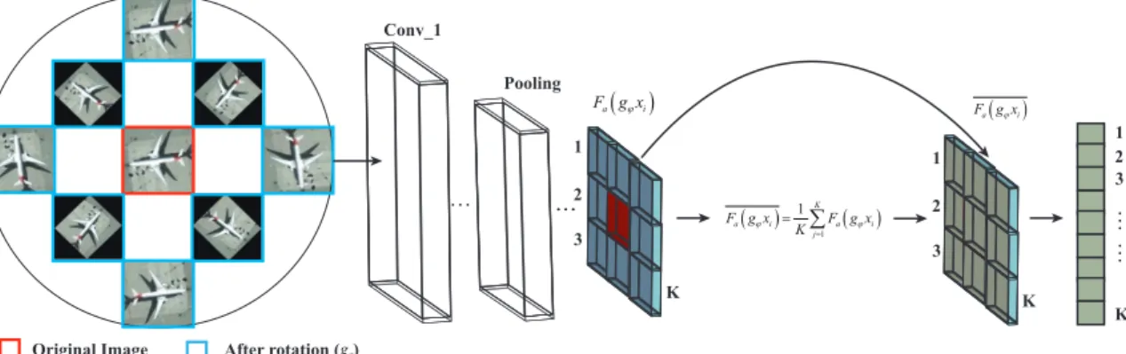
Conv_1

Pooling

  

Original Image After rotation ( )

1 3 K 2 K 1 3 2 K 1 3 2   gϕ ( ) a i F g xϕ ( ) ( ) 1 1 K a i a i j F g x F g x K ϕ ϕ = = ∑ ( ) a i F g xϕ

Figure 2.The detailed architecture of the rotation-insensitive convolutional channel features.

Conv_3 256 56 56 224 224 3 VGG-16

through Conv_3 layer

256 28 28 Conv:1 1 128× × Conv:1 1 128 / 3 3 192× × × × Conv:1 1 32 / 5 5 96× × × × Pooling:3 3 32 /1 1 64× × × × 480 28 28 480 14 14 Pooling:max 512 14 14 Conv:1 1 192× × Conv: Conv: Pooling:1 1 16 / 5 5 483 3 32 /1 1 64× × × × × × × × 1 1 96 / 3 3 208× × × × 512 7 7 Pooling:max ( ) 0 1 g x ( ) ( 0 1) a F g x _{( ( ))} 1 a F g xφ RI featu re maps RI featu re maps RI featu re maps 3 3 3 3 512 3 3 1 Pos Neg 1 Pos Neg 9 512× 1 Pos Neg 9 512× 9 512× 512 512 ACF/Deconv ACF/Deconv ACF/Deconv Detail

Figure 3.The illustration of multi-scale convolutional channel features. The features are learned by them passing through a VGG-16 network and an additional seven-layer network with an inception module. The specific implementation details are shown in the figure. To facilitate the effective detection of objects with different sizes, we generated the rotation-insensitive (RI) features at different scales. More specifically, the features in the shallow layer were applied to small-scale objects while deeper features were used for large-scale ones.

In the next step, considering that the loss function of the boosting decision tree is an exponential loss function, we adopted a probabilistic outlier model which is tightly integrated into the learning algorithms in order to minimize the error caused by manually annotated labels, among other factors,

as shown with the yellow line in Figure1. Lastly, in the detection phase, given a new test image, a

fast feature pyramid generated by a power law was used to learn the low-level feature maps and classify each sliding window to generate its class and bounding box. It is worth mentioning that the

power law [33] on the scale was used to accelerate the feature pyramid generation, whose details are

introduced in Section2.3.

2.1. Robust Low-Level Feature Generation

2.1.1. Rotation-Insensitive Feature Representation

CNN is sensitive to direction variations when attempting to recognize the objects of interest.

Following the architecture of [23], we propose to augment the data by rotating the training samples

with multiple rotation angles and by horizontally flipping them to become mirror images. Then, we embedded a regularized constraint term into the objective function of the network model, which

explicitly forces the feature representation of the training samples before and after rotation to

map closely to each other, marking the learned features rotation-insensitive. Figure2illustrates

the architecture for extracting rotation-insensitive convolutional channel features. The resulting regularized term can be formulated by

RC(X,gφX) = 1

2N_x

∑

i∈X

kFa(xi)−Fa(gφxi)k22, (1)

whereXis the samples before rotation,gφXis the samples after rotation (In theory, more rotation

angles should provide a better result. We found, however, that this could weigh the network down and degrade the performance. In our case, we empirically and experimentally determined the number of

rotation angles ranging from 0◦to 180◦at a 45◦interval.), and N is the total number of initial training

samples inX.Fa(xi)represents the feature maps of the specific layer;Fa(gφxi)represents the average

feature maps on this layer forKdirectional samples attached to each sample, and it is defined as

Fa(gφxi) = 1 K K

∑

whereKis the total number of rotation transformations for eachxi ∈X.

Obviously, the specific feature maps can be approximated as the rotation-insensitive feature maps

when Equation (1) takes the minimum value. To this end, a new loss function with a regularization

constraint term is defined by the following formula. It is noted that we mark the weight here asnetWI

so as to distinguish it from the weight of AdaBoost.

J(θ,ϕ,netWI,BI) =min(JB(θ,ϕ) +λRC(X,gφX)), (3)

wherenetWI =netw1,netw2, ...,netwa,BI=b1,b2, ...,ba,θandϕ. The first termJB(θ,ϕ)in Equation (3)

is the additive model of exponential loss function. It is designed to minimize classification errors for a given training samples and is computed by

JB(θ,ϕ) =min θ,ϕ n

∑

whereϕ,θdenotes a subclassifier and its weight;ω_ei =exp(−fe(x_i)y_i), ef(x_i)represents the output of

the strong classifier of the previous iteration;xiis theith sample;yiis the ground truth ofith sample.

We can easily see that the objective function defined by Equation (3) minimizes the detection loss,

including the loss of classification (the first term of Equation (3)) and the loss of automatic feature

generation (the second term of Equation (3)). In this paper, we solve this optimization problem by

using the stochastic gradient descent (SGD) method [34], which has been widely used in complicated

optimization problems, such as neural network training. 2.1.2. Multi-Scale Convolutional Channel Feature

The objects in the optical RSIs have different sizes, and the within-class object sizes differ greatly since the images are taken from a bird’s-eye view. A good descriptor should be able to tolerate different variations in object size. For feature extraction using the classic CNN, all objects have a single perceptual field on a particular layer, which will result in incomplete feature representation of multi-scale objects and reduce the generalization ability of the network. To this end, a multi-scale convolutional channel feature was designed by using low-level feature maps to detect small objects and high-level feature maps to detect large objects. Closely related to the requirements of the optical RSIs, we redesigned the parameters and layers of the network after fine-tuning. Compared with

the original deep CNNs, this can reduce at least half of the parameters. Figure3shows the detailed

2.2. Classifier Generation with Outlier Removal

The traditional end-to-end CNNs need to manually design the overweight hyperparameters, e.g., convolution kernel size, depth and width of the convolutional network, etc., which is time-consuming and laborious and, even using a pretrained network, some of the hyperparameters still need to be debugged or redesigned according to the requirements of new training samples. To address the tedious fine-tuning of high-level connections in CNN during the adaptation to various classification/regression problems, we adopted an AdaBoost method to classify and locate the low-level feature map

representations. AdaBoost [28,29], a typical boosting algorithm, iteratively selects weak learners

(binary decision trees) from a pool of weak candidates and targets the hard examples from the previous round. Compared with SGD’s use of an end-to-end CNN method, the binary decision tree has lower computation and storage costs. The number of its hyperparameters, e.g., max_depth, class_weight, etc., is much smaller than that for CNN. Using an optimized code, the training decision stump (depth = 1)

trains about 4608 features (3×3×512) and 10,000 iterations, requiring about 70 ms on a single core

computer and only about 7 ms on a 12 core computer, with no need for a graphics processing unit (GPU). It is worth noting that the boosting algorithm performs poorly on classification tasks with outliers,

and the generalization error of classifiers is constrained. The best reference [35] in 5th International

Conference on Learning Representations (ICLR2017) demonstrated that a powerful depth model can easily fit completely random pixels (for example, Gaussian noise) with almost zero training errors. However, as the noise level increases, the testing error of the classifier can severely deteriorate. To

this end, we introduced a probabilistic outlier model for weightsωusing the Gamma Mixture Model

(GaMM) [36–38], including two mixtures to represent inliers and outliers, respectively, i.e.,

p(ω|outlier∪inlier,Θ) ≈ p(oulier,Θ) +p(inlier,Θ) =p1 ωα1−1_e−ω/β1 Γ(α1)βα₁1 +p2 ωα2−1e−ω/β2 Γ(α2)βα₂2 , (5)

whereΘdenotes the parameter set

pl,αl,βl;l=1, 2 , andp1+p2=1. The Expectation-Maximization

(EM) algorithm [36,37] method was employed to estimate the parameter setΘof GaMM (please refer

to [38,39] for more details). The distribution of inlier and outlier samples can be estimated to calculate

their posterior probabilities. Theoretically, relatively large losses can be considered the outlier, which

is referred to asp(l=1). Based on the Bayesian posterior, its posterior probability is calculated by

p(l=1|ω,Θ)∝p(ω|l=1,Θ)p(l=1) = p1ωα1−1e−ω/β₁

Γ(α1)βα11

p(l=1). (6)

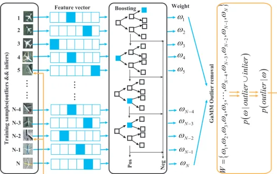
Figure4shows the details of our classifier generation. Outlier removal is performed after the

sample weight update, and the number of iterations is designed according to the actual requirements. It is tightly integrated into the AdaBoost algorithms and can fundamentally correct the bias and variance of the trained classifier caused by the outliers.

Pos Neg 1 2 3 4 5 N-4 N-3 N-2 N-1 N

Training samples(outliers && inliers)

Feature vector 1

ω

ω

ω

ω

ω

ω

ω

ω

ω

ω

{

}

,

,

,

,

,

,

,

,

,

,

W

ω

ω

ω

ω

ω

ω

ω

ω

ω

ω

=



(

)

|

p

ou

tli

er

in

lie

r

ω

∪

(

)

|

p

ou

tli

er

ω

GaMM Outlier removal

Figure 4.The detailed framework of classifier generation with outlier removal. 2.3. Detection with Power Law

Traditional detection is the output of sliding windows on the finely sampled image pyramid. It has higher accuracy but often suffers from expensive computation. The CNN-based object detection approach is the output of the object proposal, which improves the speed and performance of the method by presetting a small number of suspected candidate samples. Comparing the pros and cons

of these two approaches and inspired by Reference [40], we adopted sliding windows with a power

law [33] to accelerate the generation of fast feature pyramids. It is expressed as

P(F,s)≈Ω(R(F,s)) =R(F,s)·s−κΩ_{, (7)}

whereFis the convolutional channel feature of input image, andR(F,s)is a resampled feature ofFby

s.κis a scaling factor to be estimated. Using Equation (7), we can quickly obtain the feature pyramid

using the givenκcalculated in the training phase, and the obtained feature maps are subjected to

object detection by using the sliding windows. MsRi-CCF detects the objects on three different scales,

as illustrated in Figure3. More specifically, we set the sizes of sliding windows as 3×3, 6×3, and 3×6.

Please note that the parameter setting, e.g., the number of scales and the size of the sliding windows, is determined by minimizing the performance loss on the validation set. Since the sliding windows are performed on the shallow-layer feature maps, the amount of calculation is greatly reduced. The final detection result is non-maximum suppression and thresholded output.

2.4. A Quick Look at Illustrative Examples

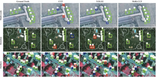
Figure5illustrates some representative examples to clarify the effectiveness and superiority of

MsRi-CCF under three different conditions. The first and second rows show the detection results with multi-scale and rotation, respectively. The original CCF not only produces a false positive (in blue) but also a false negative (in red), leading to a relatively poor detection performance. YOLO2 outperforms the CCF in the multi-scale case, although some objects are still missing. Unfortunately, both CCF and YOLO2 fail to effectively detect the rotated objects. It is obvious that compared with the above two methods, the proposed MsRi-CCF is better able to handle the multi-scaled and rotated objects. The complex scenes are prone to generate clusters of false positives and false negatives, as shown in the last

row of the CCF and YOLO2 (see Figure5), while MsRi-CCF benefits from outlier removal, reducing

Ground Truth YOLO2 MsRi-CCF 1 1 1 1 1 1 1 1 1 1 1 1 1 1 1 1 1 1 1 1 1 1 1 1 1 1 1 1 1 1 1 1 1 1 1 1 1 10 10 10 10 10 10 10 10 10 10 10 10 10 10 10 1010 10 10 10 10 10 10 10 10 10 10 10 10 10 10 10 10 10 10 10 10 10 1010 10 10 10 10 10 10 10 2 10 10 10 10 10 10 10 10 10 10 10 10 10 10 10 1010 10 10 10 10 10 10 5 10 10 10 10 10 10 10 10 10 10 10 10 10 10 10 10 1010 10 10 10 10 10 10 10 1 4 4 4 5 5 5 5 5 5 4 4 4 5 5 5 5 5 5 4 4 4 4 5 5 5 5 5 5 4 4 4 4 4 4 5 5 5 5 5 R otati on CCF M u lti -s c al e O u tl ie r s

Figure 5.Visual comparison of three different methods (CCF, YOLO2, and MsRi-CCF) with regard to multi-scale, direction variation, and outliers.

3. Experiment

3.1. Experimental Dataset

In this section, two public optical remote datasets, NWPU VHR-10 (http://www.ifp.uni-stuttgart.

de/dgpf/DKEPAllg.html) and a satellite dataset (http://ai.stanford.edu/~gaheitz/Research/TAS/),

are used to quantitatively evaluate the performances of the proposed method.

(1) NWPU VHR-10 dataset: This dataset is a very high resolution (VHR) optical remote sensing image dataset. It consists of two acquisition modes: color images with a spatial resolution of 0.5–2 m obtained from Google Earth and infrared images with a spatial resolution of 0.08 m obtained from the Vaihingen dataset (the Vaihingen data was provided by the German Society for Photogrammetry,

Remote Sensing and Geoinformation (DGPF)). (Please refer to [8,41].) In this dataset, there are

650 images with 10 class objects, namely, baseball diamond, ground track field, basketball court,

airplane, ship, storage tank, tennis court, harbor, bridge, and vehicle. Table1shows the size of each

class object.

(2) Satellite dataset: This is a small dataset of optically remotely sensed vehicles used by

Heitz et al. in ECCV 2008 [42]. The dataset was acquired from Google Earth. Each image is a

color image of 792×636, containing 1319 vehicle objects labeled manually with an average size of

45×45. The vehicle objects have a large direction variation and a small range of scale. It is noted that

the presence of obstructions and low resolution increase the difficulty of vehicle detection.

Table 1.The statistics of object size in the NWPU VHR-10 dataset.

Class Name Minimum Size Maximum Size Mean Size

Airplane 33×33 129×129 81×81 Storage tank 34×34 103×103 69×69 Ship 40×40 128×128 84×84 Vehicle 42×42 91×91 67×67 Tennis court 45×45 127×127 86×86 Baseball diamond 49×49 179×179 114×114 Basketball court 52×52 179×179 116×116 Harbor 68×68 222×222 145×145 Bridge 98×98 363×363 231×231

3.2. Experimental Setup

Due to the limited number of the training samples, data augmentation is a feasible solution for effective network training. For the two datasets, the rotation and mirror operations were performed to enlarge the training set. More specifically, we rotated the training images with different angles

ranging from 0◦ to 180◦ at a 45◦interval. We also converted the training images to the HSV (hue,

saturation, value) color space as a preprocessing step for improving the robustness to illumination and atmospheric effects. The negative images were randomly selected from the set of images without a detected object in the current class. In our work, 60% of the samples were assigned to the training set and the rest compose the test set. To stably evaluate the performance of the proposed method, we conducted five-fold cross-validation and report an average result across the folds below.

In addition, all the experiments were implemented using the TensorFlow framework and carried out by a PC with an Intel single Core i7 CPU, NVIDIA GTX-1070 GPU (4 GB memory), and 32 GB RAM. The PC operating system is Ubuntu 15.04.

3.3. Evaluation Criteria

Analogous to an evaluation method for object detection, the precision–recall curve (PRC) and average precision (AP) were adapted to quantitatively evaluate the detection performances. More precisely, when the intersection-over-union (IoU) overlap rate between the detected bounding box and the ground truth exceeds 50%, the detection result is the predicted result (true positive (TP)). If multiple detection results overlap with the same ground truth, the highest overlap rate is the predicted result; otherwise, a false negative (FN) results. Therefore, the final precision (P) is computed

by TP

TP+FP, and the recall (R) rate is

TP

TP+FN. APis a global indicator to assess the performance

of the method. Moreover, we evaluated the detection performance of the proposed MsRi-CCF in comparison with seven state-of-the-art baselines.

• The collection of part detector (COPD) [41] is composed of a set of representative and

discriminative linear support vector machine (SVM) classifier part detectors. In our experiments, we adopted the original setting for fair comparison.

• The Exemplar-SVM detector [43] adopts template integration instead of a single template to

realize object detection. In our experiments, we used a sizing heuristic method for each sample to create an 8-pixel-sized descriptor based on its ground truth bounding box.

• The fast feature pyramid [40] is a fast object detection framework which estimates features at

a coarsely sampled set of scales. In our experiments, this applies to all three channel features, namely, color, gradient magnitude, and gradient orientation.

• The convolutional channel feature (CCF) [30] is a light-weight model with deep representations.

In our experiments, we used a VGG-16 model as the feature extractor.

• Bag of visual words and SVM classifier (BOW-SVM) [44] is a simplified representation achieved

by transforming the text into a “bag of words”. In our experiments, we still represented each image block as a histogram with a similar visual vocabulary generated by a k-means algorithm.

• You only look once (YOLO1) [45] performs the object detection task, which consists of determining

the location on the image where certain objects are present, as well as classifying those objects with a single feed-forward convolutional network. In our experiments, we adopted the detection network from darknet-24, which has 24 convolutional layers followed by 2 fully connected layers.

• YOLO9000 (YOLO2) [46] is an enhancement of YOLO1. It removes the fully connected layers

and uses anchor boxes to predict bounding boxes. In our experiments, we adopted the detection network from darknet-19, which has 19 convolutional layers.

3.4. Parameter Setting

In general, the hyperparameters in MsRi-CCF are determined by maximizing the performance on the validation set. Besides that, we also provide a more specific discussion and analysis on the selection of feature maps and the rate of outlier removal in the following subsections.

3.4.1. Feature Map Selection

The distinguishability of the feature maps is very important for designing a classifier. The depth of the network, the number of parameters, and the convergence speed of parameter estimation all directly affect the speed and performance of the network. However, scale and direction variation of optical RSIs make it difficult to directly fine-tune using pretrained networks of natural scene images. Therefore, an additional seven-layer network was designed to reduce the sensitivity of the network to scale and direction variation, thereby improving the generalization capabilities of the network.

An inception module with 1×1 convolution [47] was also introduced to improve the expressive ability

of the network and extend the network’s depth and width without increasing computational costs. We used Rectified Linear Unit (ReLU) as the activation function. It is fast, promotes sparsity in the

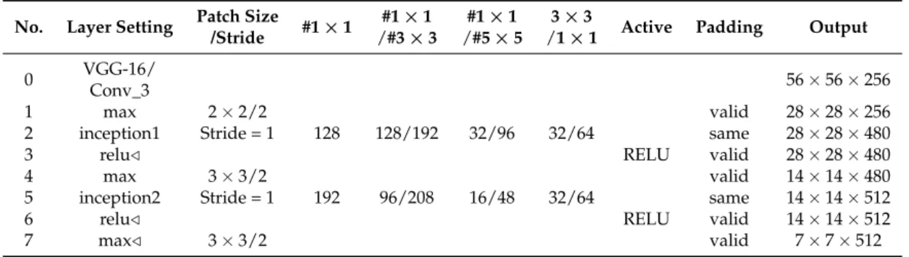
network, and reduces the likelihood of a vanishing gradient. Table2demonstrates the structure of

the convolutional feature extractor, which has eight convolutional layers in total, where theconv_3 of

VGG-16 is applied to the first layer and the others are an additional seven-layer network, and/stands

for the rotation-insensitive descriptor.

Table 2.The network architecture in feature extraction of our MsRi-CCF.

No. Layer Setting Patch Size #1×1 #1×1 #1×1 3×3 Active Padding Output /Stride /#3×3 /#5×5 /1×1

0 VGG-16/ 56×56×256

Conv_3

1 max 2×2/2 valid 28×28×256

2 inception1 Stride = 1 128 128/192 32/96 32/64 same 28×28×480

3 relu/ RELU valid 28×28×480

4 max 3×3/2 valid 14×14×480

5 inception2 Stride = 1 192 96/208 16/48 32/64 same 14×14×512

6 relu/ RELU valid 14×14×512

7 max/ 3×3/2 valid 7×7×512

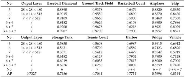
The distinguishability of feature maps in automatic feature learning determines the performance of object detection and classification. Theoretically, as the network deepens, the local distinguishability becomes greater. Considering the large-scale variation of objects in optical RSIs, we chose 3 medial layers as candidate low-level features to realize a good balance between feature representativeness and generalization ability. Since the deeper feature maps have weaker resolutions, they were considered for detecting objects with large sizes, while higher resolution layers were considered for detecting

small-scale objects. Tables3and4give the precision of each class in the NWPU VHR-10 dataset and

the precision for one class in the satellite dataset. The following observations are made. (1) Compared

with the optimal precision of single feature maps, the AP of the 3+6+7th layer increased by about

5% with the NWPU VHR-10 dataset, but on the satellite dataset, the AP is just slightly improved. This result is due to the fact that the scale variation of the objects in the satellite dataset is small. (2) For the

storage tank, tennis court, and vehicle, the precision of the 3rdlayer is higher than the other layers.

This is because their appearance and size are relatively simple. Otherwise, for the baseball diamond and ground track field, the highest precision is in the 7th layer. (3) Compared with the NWPU VHR-10 dataset, the precision of the vehicle in the satellite dataset is higher, which is due to the high degree of similarity between the vehicles and their spatial semantic information, which is relatively simple.

Table 3.The precision of three intermediate layers for the NWPU VHR-10 dataset.

No. Ouput Layer Baseball Diamond Ground Track Field Basketball Court Airplane Ship

3 28×28×480 0.8890 0.9378 0.6479 0.8820 0.8630 6 14×14×512 0.9015 0.9550 0.6890 0.8870 0.8430 7 7×7×512 0.9109 0.9660 0.5900 0.8469 0.7530 3 + 6 / 0.9182 0.9626 0.6159 0.8900 0.7986 6 + 7 / 0.9200 0.9678 0.6216 0.8921 0.8029 3 + 6 + 7 / 0.9207 0.9700 0.7900 0.8957 0.8571

No. Output Layer Storage Tank Tennis Court Harbor Bridge Vehicle

3 28×28×480 0.5850 0.5608 0.6987 0.6915 0.6912 6 14×14×512 0.5621 0.5790 0.6589 0.7123 0.6890 7 7×7×512 0.5571 0.5412 0.6479 0.6547 0.5919 3 + 6 / 0.6182 0.6127 0.7952 0.7900 0.7128 6 + 7 / 0.6019 0.6055 0.7817 0.8000 0.7000 3 + 6 + 7 / 0.6276 0.6250 0.8002 0.8259 0.7420 No. 3 6 7 3 + 6 6 + 7 3 + 6 + 7 AP 0.7327 0.7486 0.7041 0.7714 0.7696 0.8144

Table 4.The precision of three medial layers for the satellite dataset.

Class 3 6 7 3 + 6 6 + 7 3 + 6 + 7

Vehicle 0.8951 0.8720 0.7216 0.9011 0.8259 0.9019

3.4.2. Outlier Removal in Classifier Generation

The ground truth in feature maps is the mapping of the ground truth in the original image. It is used as the positive sample input of the AdaBoost classifier. We sample or interpolate the feature maps to ensure the size consistency between objects of the same class. The addition of outlier removal can further optimize the training samples and remove the hard samples to obtain a “clean” training set. For the details on the parameter estimation and convergence rate of the GaMM distribution, refer to

Reference [38,39]. It is worth noting that the proportion of outliers in this paper is unknown, and we

did not add extra outliers. Table5shows the AP under each iteration. It is shown that both datasets

achieve optimal performance after the first iteration. From the conclusion in Reference [38], it is shown

that the outlier ratio is less than 5%, which can be removed with only one iteration. Also, since the number of training samples is too small, as iterations increases, inliers decrease, directly affecting the performance of the classifier, especially for satellite dataset.

Table 5.Comparison of average precision (AP) under different iteration times of the Gamma Mixture Model (GaMM) distribution with the two datasets.

Dataset 0 1 2 3 4

NWPU VHR-10 0.8044 0.7500 0.7000 0.6890 0.7429

Satellite 0.9019 0.8212 0.7800 0.7259 0.6928 3.5. Performance Analysis with the NWPU VHR-10 Dataset

For training samples larger than 224×224×3, we cut them into an image block set of this size

and recorded the coordinates of the diagonal. In order to prevent the object from splitting, we set an overlap for objects of the same class that were larger than the average size for that class. For fairness, we adopted the same preprocessing to ensure sample consistency for all methods. Specifically, our

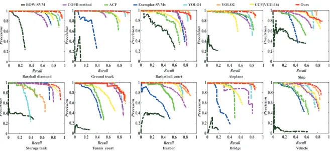
method was computed with optimal parameters and feature maps. Figure6shows the PRC of the

eight methods. It is shown that the precision and recall of three classes, namely, baseball diamond, ground track field, and airplane, are higher using all the listed methods. This occurs because their appearance, structure, and local semantic information are relatively distinguishable.

Baseball diamond

Ours COPD method

BOW-SVM ACF Exemplar-SVMs YOLO1 YOLO2

Airplane

Storage tank Tennis court

Ground track Basketball court Ship

Harbor Bridge Vehicle

CCF(VGG-16) 0 0.2 0.4 0.6 0.8 1 Recall 0 0.2 0.4 0.6 0.8 1 Precision 0 0.2 0.4 0.6 0.8 1 Recall 0 0.2 0.4 0.6 0.8 1 Precision 0 0.2 0.4 0.6 0.8 1 Recall 0 0.2 0.4 0.6 0.8 1 Precision 0 0.2 0.4 0.6 0.8 1 Recall 0 0.2 0.4 0.6 0.8 1 Precision 0 0.2 0.4 0.6 0.8 1 Recall 0 0.2 0.4 0.6 0.8 1 Precision 0 0.2 0.4 0.6 0.8 1 Recall 0 0.2 0.4 0.6 0.8 1 Precision 0 0.2 0.4 0.6 0.8 1 Recall 0 0.2 0.4 0.6 0.8 1 Precision 0 0.2 0.4 0.6 0.8 1 Recall 0 0.2 0.4 0.6 0.8 1 Precision 0 0.2 0.4 0.6 0.8 1 Recall 0 0.2 0.4 0.6 0.8 1 Precision 0 0.2 0.4 0.6 0.8 1 Recall 0 0.2 0.4 0.6 0.8 1 Precision

Figure 6.Precision–recall curve (PRC) of the proposed method and seven competitive methods using the NWPU VHR-10 dataset for 10 object classes.

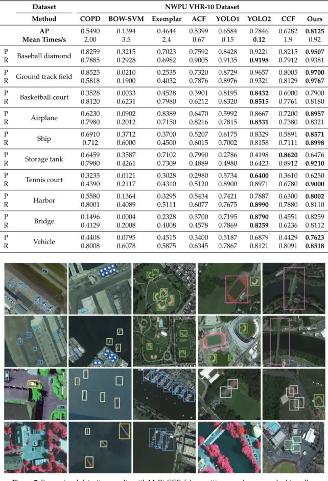
Table6lists the quantitative results of the eight studied methods in terms of four different metrics:

AP value, running time, as well as precision and recall for each class, while Figure7visually highlights

some detection results for the 10 classes using the NWPU VHR-10 dataset, where each class is marked in a different color, the yellow bounding box shows false detection, and the red bounding box shows missed detection. We can conclude the following. (1) The AP value of BOW-SVM is lower than that of the other methods. This is because BOW-SVM represents each image block as a histogram of a similar visual vocabulary generated by the K-means algorithm. By ignoring the relationship of the spatial structures among local features, it can only detect objects with simple shapes, such as baseball diamond, storage tank, and ship. Although Exemplar-SVM designed the classifier for each class respectively, the generalization ability of the histogram of gradient (HOG) descriptor is sensitive to the deformation. Similarly, it is not surprising that the detection performance of the COPD algorithm and ACF are also limited by the feature representation capabilities of the HOG. (2) YOLO1 is the fastest approach, but it has a certain trade-off with detection accuracy. It has weak generalization ability for a large scale range and rotation variation of objects under a complex background. Compared with YOLO1, although YOLO2 uses multi-scale images for training and convolutional feature maps for testing, the AP value is upgraded from 0.6584 to 0.7846. However, for different aspect ratios of the same object class, the generalization ability of the algorithm is greatly downgraded. (3) Compared with the CCF, which directly investigates the VGG-16 model, the addition of rotation-insensitive descriptor and multi-scale aggregated descriptor achieves about 0.2 gains in terms of mean AP. This shows that our method is effective for detecting objects in multi-scale optical RSIs. For feature generation, we chose the convolutional layer to introduce into the next feature learning. It is more intuitive to adopt fully connected layers to perform classification and detection; however, (1) the convolutional layer is a local connection and is suitable for the input of any size, and the fully connected layer is a global connection; (2) compared with the full-connection layer, the convolutional layer shares a large number of calculations, and it can substantially reduce the amount of calculation. Moreover, the feature learning (such as edge removal and dimensionality reduction) on feature maps was added to train our detector with the boosting decision tree. This idea was inspired by the actual algorithm

Table 6. Quantitative performance comparisons and average running time for the NWPU VHR-10 dataset. The optimal value is shown in bold.

Dataset NWPU VHR-10 Dataset

Method COPD BOW-SVM Exemplar ACF YOLO1 YOLO2 CCF Ours

AP 0.5490 0.1394 0.4644 0.5399 0.6584 0.7846 0.6282 0.8125 Mean Times/s 2.00 3.5 2.4 0.67 0.15 0.12 1.9 0.92 P Baseball diamond 0.8259 0.3215 0.7023 0.7592 0.8428 0.9221 0.8215 0.9507 R 0.7885 0.2928 0.6982 0.9005 0.9135 0.9198 0.7912 0.9381 P

Ground track field 0.8525 0.0210 0.2535 0.7320 0.8729 0.9657 0.8005 0.9700

R 0.5818 0.1900 0.4032 0.7876 0.8976 0.9321 0.8129 0.9767 P Basketball court 0.3528 0.0033 0.4528 0.3901 0.8195 0.8432 0.6000 0.7900 R 0.8120 0.6231 0.7980 0.6212 0.8320 0.8515 0.7761 0.8180 P Airplane 0.6230 0.0902 0.8389 0.6470 0.5992 0.8667 0.7200 0.8957 R 0.7980 0.2012 0.7150 0.8216 0.7815 0.8531 0.7380 0.8321 P Ship 0.6910 0.3712 0.3700 0.5207 0.6175 0.8329 0.5891 0.8571 R 0.712 0.6000 0.4500 0.6015 0.7002 0.8158 0.7111 0.8998 P Storage tank 0.6459 0.3587 0.7102 0.7990 0.2786 0.4198 0.8620 0.6476 R 0.7980 0.4261 0.7309 0.4889 0.4980 0.6423 0.8912 0.9210 P Tennis court 0.3235 0.0121 0.3028 0.2980 0.5734 0.6400 0.3610 0.6250 R 0.4390 0.2117 0.4310 0.5120 0.8900 0.8971 0.6780 0.9000 P Harbor 0.5580 0.1364 0.3295 0.5434 0.7421 0.7887 0.6300 0.8002 R 0.8001 0.4089 0.5111 0.6077 0.7675 0.8990 0.7880 0.8110 P Bridge 0.1496 0.0004 0.2328 0.3700 0.7195 0.8790 0.4551 0.8259 R 0.4129 0.2008 0.4008 0.4578 0.7869 0.8259 0.6236 0.8112 P Vehicle 0.4408 0.0795 0.4515 0.3400 0.5187 0.6879 0.4429 0.7623 R 0.8008 0.6078 0.5875 0.6345 0.7867 0.8121 0.8091 0.8518

Figure 7.Some visual detection results with MsRi-CCF; false positive samples are marked in yellow and true positives are in the other colors.

As expected, the proposed MsRi-CCF obtains the best detection performance in terms of mean AP, despite having a relatively low running speed compared with YOLO-like methods. This can be well explained by our targeted-designed end-to-end feature learning. More specifically, the multi-scaled design effectively improves the detection performance, particularly for those with irregular sizes

(e.g.,Ground track field), while the embedding of rotation-invariant features is greatly conducive to

detecting the objects sensitive to direction (e.g.,Airplane, Vehicle). Moreover, the robustness of our

detector is capable of further being enhanced, after the learned features pass through the outlier

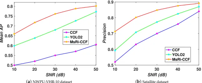
removal module. An illustrative example can be found in Figure8. Additionally, MsRi-CCF performs

more efficiently, with a decrease of about 1 s per image, than the CCF with the great support of fast feature pyramid modeling and our proposed multi-scale strategy.

10 20 30 40 50 SNR (dB) 0.5 0.55 0.6 0.65 0.7 0.75 0.8 Mean AP CCF YOLO2 MsRi-CCF (a)NWPU-VHR-10 dataset 10 20 30 40 50 SNR (dB) 0.5 0.6 0.7 0.8 0.9 Precision CCF YOLO2 MsRi-CCF (b)Satallite dataset Figure 8.Evaluation of robustness to noise of the MsRi-CCF framework. 3.6. Performance Analysis on Satellite Dataset

Figure9shows the PRC of the eight different detection algorithms, and Table7correspondingly

lists the running times, as well as precision (P value) and recall (R value). Visually, a showcase is also

given in Figure10. The green, red, and blue bounding boxes represent the true positive, false positive,

and missed detection, respectively.

0

0.2

0.4

0.6

0.8

1

Recall

0

0.2

0.4

0.6

0.8

1

Precision

COPD method BOW-SVM

Exemplar-SVMs

YOLO1ACF YOLO2

CCF(VGG-16)

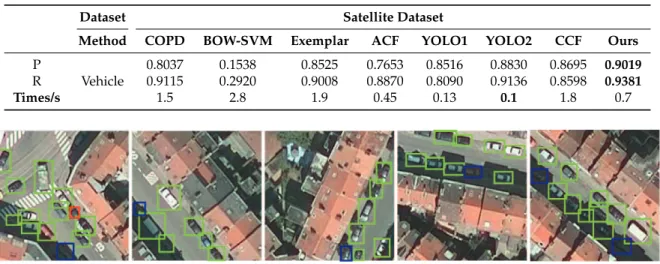
Table 7. Quantitative performance comparisons and running time with the satellite dataset. The optimal value is shown in bold.

Dataset Satellite Dataset

Method COPD BOW-SVM Exemplar ACF YOLO1 YOLO2 CCF Ours

P

Vehicle

0.8037 0.1538 0.8525 0.7653 0.8516 0.8830 0.8695 0.9019

R 0.9115 0.2920 0.9008 0.8870 0.8090 0.9136 0.8598 0.9381

Times/s 1.5 2.8 1.9 0.45 0.13 0.1 1.8 0.7

Figure 10.A showcase of MsRi-CCF with the satellite dataset (false detection in red, true positive in green, and missed detection in blue).

Overall, BOW-SVM and Exemplar-SVM are only robust to vehicles with similar shape variation, and its generalization ability is relatively weak. The HOG descriptor used in the ACF and COPD algorithm is sensitive to object rotation, which leads to a limited precision. YOLO2 is an improved version of YOLO1, which enhances the generalization of YOLO1 for scale transformation and direction variation. Unfortunately, the multi-resolution objects and the narrow distance between them degrade the detection performance of YOLO-based networks. In the CCF, the VGG-16 network framework is explored for feature extraction, yet it is sensitive to multi-scale and multi-direction effects in optical RSIs and cannot achieve desirable detection results. Not surprisingly, the performance of the MsRi-CCF is superior to that of the others. Similar to the NWPU VHR-10 dataset, the learned features in MsRi-CCF is robust against rotation behavior with the satellite dataset, as the rotation-insensitive term is regularized in our network, while the use of multi-scaled feature maps can reduce the rate of missed detection of the larger or smaller objects. It should be noted that the biggest challenge with this dataset is the black vehicles that are obscured by the tree, as they are difficult to distinguish from the ground. A straightforward way to address this problem is to train a more robust classifier by removing the “bad” samples (outliers), just as the outlier removal was used in our framework. Furthermore, although MsRi-CCF cannot beat the YOLO-based approaches in running speed, it is much faster than the original CCF and some previous methods owing to our efficiency-oriented improvement (e.g., fast feature pyramid, multi-scale feature design).

3.7. Robustness Analysis to Noises

To intuitively evaluate the robustness of MsRi-CCF, we investigated the detection performances of three representative algorithms on two datasets by adding Gaussian white noise in different ranges

of signal-to-noise-ratios (SNRs), from 10 to 50 dB with a 10 dB interval. As can be seen in Figure8,

the CCF sharply degrades in performance with a decrease in SNR and is more sensitive to noise attack than YOLO2. On the other hand, there is a comparatively stable trend in MsRi-CCF. This demonstrates that the outlier removal strategy could play a role in correcting the decision boundary to some extent.

3.8. Discussion on the Selection of Feature Extractor in MsRi-CCF

The feature extractor in the proposed MsRi-CCF consists of a deep neural network, such as

AlexNet, VGG, or ResNet. Table8lists the performance comparisons for the three network architectures

used as the feature extractor for the satellite and NWPU VHR-10 datasets. As observed, AlexNet runs faster than the other two (VGG-16 and ResNet-34), yet its detection precision is considerably lower

than theirs. It should be noted that VGG-16 and ResNet-34 yield similar performances. This might be explained by the possible fact that, in our case, the features extracted by VGG-16 are discriminative enough to achieve an object detection success which is comparable to that of ResNet-34. We have to emphatically clarify again that the motivation and goal of this paper are to improve the robustness to scaling and rotation in geospatial object detection rather than greatly enhance feature representation ability. For simplicity, the VGG-16 network was applied in our framework.

Table 8.Precision comparisons of the proposed MsRi-CCF using three different network architectures as the feature extractor. The best results are shown in bold.

Dataset Network AlexNet VGG-16 ResNet-34

Satellite dataset Vehicle 0.7213 0.9019 0.8895

Times/s 0.56 0.7 0.73

NWPU VHR-10 dataset

Baseball diamond 0.7525 0.9507 0.9428

Ground track field 0.7982 0.9700 0.9612

Basketball court 0.5629 0.7900 0.8520 Airplane 0.5214 0.8957 0.9121 Ship 0.6720 0.8571 0.8610 Storage tank 0.4790 0.6476 0.6428 Tennis court 0.5136 0.6250 0.6612 Harbor 0.6087 0.8002 0.7926 Bridge 0.5961 0.8259 0.8424 Vehicle 0.5908 0.7623 0.7420 AP 0.6095 0.8125 0.8210 Mean Times/s 0.70 0.92 0.97 4. Conclusions

In reality, geospatial object detection ability remains limited due to multi-resolution and rotation-sensitive properties of objects. To advance network training toward more robust and accurate object detection, we propose a novel object detection framework, called MsRi-CCF. MsRi-CCF aims to learn rotation-insensitive feature representation in a multi-scale fashion. With the outlier removal strategy, some negative detection results can be effectively removed, leading to further improvement in terms of detection performance. Extensive experiments conducted on the NWPU VHR-10 dataset and satellite dataset show the superiority and effectiveness of our method in comparison with several state-of-the-art baselines. We have to admit, however, that although MsRi-CCF performs better than YOLO2 by around 3% in terms of AP and precision, there is still room for improvement in computation time. For this objective, we will attempt to design a novel detection framework that is more effective and efficient in the future by introducing some fast modules for object modeling and localization.

Author Contributions: Conceptualization, X.W. and D.H.; methodology, X.W. and D.H.; software, X.W.; validation, X.W., D.H. and P.G.; formal analysis, P.G. and W.L.; investigation, D.H.; writing—original draft preparation, X.W. and D.H.; writing—review and editing, X.W., D.H., P.G. and W.L.; visualization, X.W.; supervision, P.G., W.L. and R.T.; project administration, R.T.; funding acquisition, R.T.

Funding:This research was supported, in part, by the National Natural Science Foundation of China under Grant 61331021 and Grant 61421001, and, in part, by the National Natural Science Foundation of China (U1833203). Acknowledgments: The authors would like to thank the Key Laboratory of Information Fusion Technology, Ministry of Education at the University of Northwestern Polytechnical for providing the NWPU VHR-10 dataset and to thank the Stanford Artificial Intelligence Laboratory for providing the satellite dataset. The authors would like to express their appreciation to Prof. Piotr Dollar for providing MATLAB codes for fast pyramid feature and to thank Google for opening the TensorFlow Object Detection API.

References

1. Hong, D.; Yokoya, N.; Xu, J.; Zhu, X. Joint & Progressive Learning from High-Dimensional Data for Multi-Label Classification. In Proceedings of the European Conference on Computer Vision (ECCV) (2018), Munich, Germany, 8–14 September 2018; pp. 469–484.

2. Yokoya, N.; Ghamisi, P.; Xia, J. Open data for global multimodal land use classification: Outcome of the 2017 IEEE GRSS Data Fusion Contest.IEEE J. Sel. Top. Appl. Earth Obs. Remote Sens.2018,11, 1363–1377. [CrossRef]

3. Hong, D.; Yokoya, N.; Zhu, X. Learning a Robust Local Manifold Representation for Hyperspectral Dimensionality Reduction.IEEE J. Sel. Top. Appl. Earth Obs. Remote Sens.2017,10, 2960–2975. [CrossRef] 4. Benediktsson, J.A.; Chanussot, J.; Moon, W.M. Very high-resolution remote sensing: Challenges and

opportunities.Proc. IEEE2012,100, 1907–1910. [CrossRef]

5. Tochon, G.; Chanussot, J.; Dalla Mura, M.; Bertozzi, A.L. Object tracking by hierarchical decomposition of hyperspectral video sequences: Application to chemical gas plume tracking.IEEE Trans. Geosci. Remote Sens. 2017,55, 4567–4585. [CrossRef]

6. Hong, D.; Yokoya, N.; Chanussot, J.; Zhu, X. Learning a low-coherence dictionary to address spectral variability for hyperspectral unmixing. In Proceedings of the 24th IEEE International Conference on Image Processing (ICIP) (2017), Beijing, China, 17–20 September 2017; pp. 235–239.

7. Hong, D.; Yokoya, N.; Chanussot, J.; Zhu, X. An Augmented Linear Mixing Model to Address Spectral Variability for Hyperspectral Unmixing.arXiv2018, arXiv:1810.12000.

8. Cheng, G.; Han, J.W. A Survey on Object Detection in Optical Remote Sensing Images.ISPRS J. Photogramm. Remote Sens.2016,117, 11–28. [CrossRef]

9. Han, J.; Zhang, D.; Cheng, G.; Liu, N.; Xu, D. Advanced deep learning techniques for salient and category-specific object detection: A survey.IEEE Signal Process. Mag.2018,35, 84–100. [CrossRef]

10. Uijlings, J.R.; Van De Sande, K.E.; Gevers, T.; Smeulders, A.W. Selective search for object recognition.Int. J. Comput. Vis.2013,104, 154–171. [CrossRef]

11. Xu, X.; Li, W.; Ran, Q.; Du, Q.; Gao, L.; Zhang, B. Multisource Remote Sensing Data Classification Based on Convolutional Neural Network.IEEE Trans. Geosci. Remote Sens.2018,56, 937–949. [CrossRef]

12. Zhang, M.; Li, W.; Du, Q. Diverse Region-Based CNN for Hyperspectral Image Classification.IEEE Trans. Image Process.2018,27, 2623–2634. [CrossRef]

13. Chen, Y.; Jiang, H.; Li, C.; Jia, X.; Ghamisi, P. Deep feature extraction and classification of hyperspectral images based on convolutional neural networks. IEEE Trans. Geosci. Remote Sens. 2016,54, 6232–6251. [CrossRef]

14. Chen, Y.; Zhu, L.; Ghamisi, P.; Jia, X.; Li, G.; Tang, L. Hyperspectral images classification with Gabor filtering and convolutional neural network.IEEE Geosci. Remote Sens. Lett.2017,14, 2355–2359. [CrossRef]

15. Ghamisi, P.; Yokoya, N. IMG2DSM: Height Simulation From Single Imagery Using Conditional Generative Adversarial Net.IEEE Geosci. Remote Sens. Lett.2018,15, 794–798. [CrossRef]

16. Lee, H.; Grosse, R.; Ranganath, R.; Ng, A. Unsupervised learning of hierarchical representations with convolutional deep belief networks.Commun. ACM2011,54, 95–103. [CrossRef]

17. Yosinski, J.; Clune, J.; Nguyen, A.; Fuchs, T.; Lipson, H. Understanding Neural Networks Through Deep Visualization. In Proceedings of the 31st International Conference on Machine Learning (ICML), Lille, France, 6–11 July 2015; pp. 1–12.

18. Zeiler, M.D.; Fergus, R. Visualizing and Understanding Convolutional Networks. In Proceedings of the 13th European Conference on Computer Vision (ECCV), Zurich, Switzerland, 6–12 September 2014; pp. 818–833. 19. Cheng, L.; Liu, X.; Li, L.L.; Jiao, L.C.; Tang, X. Deep Adaptive Proposal Network for Object Detection in

Optical Remote Sensing Images.IEEE Trans. Geosci. Remote Sens. Mag.2008,10, 142–149.

20. Deng, Z.; Sun, H.; Zhou, S.; Zhao, J.; Lei, L. Multi-scale object detection in remote sensing imagery with convolutional neural networks.ISPRS J. Photogramm. Remote Sens.2018,10, 142–149. [CrossRef]

21. Wu, Z.H.; Chen, X.N.; Gao, Y.M.; Li, Y.T. Rapid Target Detection in High Resolution Remote Sensing Images Using YOLO Model.Int. Arch. Photogramm. Remote Sens. Spat. Inf. Sci. 2018,XLII-3, 1915–1920. [CrossRef] 22. Xia, G.S.; Bai, X.; Ding, J.; Zhu, Z.; Belongie, S.; Luo, J.B.; Datcu, M.H.; Pelillo, M.; Zhang, L.P. DOTA: A Large-scale Dataset for Object Detection in Aerial Images. In Proceedings of the 2018 IEEE Conference on Computer Vision and Pattern Recognition (CVPR), Salt Lake City, UT, USA, 18–22 June 2018; pp. 1–10.

23. Cheng, G.; Zhou, P.; Han, J. Learning rotation-invariant convolutional neural networks for object detection in vhr optical remote sensing images.IEEE Trans. Geosci. Remote Sens. Mag.2016,54, 7405–7415. [CrossRef]

24. Chen, X.; Xiang, S.; Liu, C.L.; Pan, C.H. Vehicle detection in satellite images by hybrid deep convolutional neural networks.IEEE Trans. Geosci. Remote Sens. Lett.2014,11, 1797–1801. [CrossRef]

25. Chen, X.; Xiang, S.; Liu, C.L.; Pan, C.H. Vehicle detection in satellite images by parallel deep convolutional neural networks. In Proceedings of the 2nd IAPR Asian Conference on Pattern Recognition (ACPR) (2013), Okinawa, Japan, 5–8 November 2013; pp. 181–185.

26. Krizhevsky, A.; Sutskever, I.; Hinton, G.E. ImageNet Classification with Deep Convolutional Neural Networks. In Proceedings of the 25th International Conference on Neural Information Processing Systems (NIPS) (2012), Lake Tahoe, NV, USA, 3–6 December 2012; pp. 1097–1105.

27. He, K.M.; Zhang, X.Y.; Ren, S.Q.; Sun, J.; Torr, P. Deep Residual Learning for Image Recognition. In Proceedings of the IEEE Conference on Computer Vision and Pattern Recognition (CVPR) (2016), Las Vegas, NV, USA, 27–30 June 2016; pp. 770–778.

28. Breiman, L. Rejoinder: Arcing classifiers.Ann. Stat.1998,26, 841–849. 29. Breiman, L. The state of boosting.Comput. Sci. Stat.2001,31, 1722–1731.

30. Yang, B.; Yan, J.J.; Lei, Z.; Li, S. Convolutional Channel Features. In Proceedings of the International Conference on Computer Vision (ICCV) (2015), Santiago, Chile, 11–18 December 2015; pp. 82–90.

31. Moghimi, M.; Belongie, S.; Saberian, M.; Yang, J. Convolutional Channel Features. In Proceedings of the 27th British Machine Vision Conference (2016), York, UK, 19–22 Sepember 2016; pp. 1–13.

32. Wu, C.H.; Gan, W.H.; Lan, D.; Jay, C.C. Boosted Convolutional Neural Networks (BCNN) for Pedestrian Detection. In Proceedings of the IEEE Winter Conference on Applications of Computer Vision (WACV) (2017), Santa Rosa, CA, USA, 24–31 March 2017; pp. 540–549.

33. Ruderman, D.L.; Bialek, W. Statistics of Natural Images: Scaling in the Woods.Phys. Rev. Lett.1994,73, 814–817. [CrossRef] [PubMed]

34. Rumelhart, D.E.; Hinton, G.E.; Williams, R.J. Learning representations by back-propagating errors.Nature 1986,323, 533–536. [CrossRef]

35. Zhang, C.; Bengio, S.; Hardt, M.; Recht, B.; Vinyals, O. Understanding deep learning requires rethinking generalization. In Proceedings of the European Conference on Computer Vision (ICLR) (2017), Toulon, France, 24–26 April 2017; pp. 1–14.

36. KapoorEmail, A.; Hemani, H.; Sakthivel, N.; Chaturvedi, S. Mpi implementation of expectation maximization algorithm for gaussian mixture models. In Proceedings of the 12th Annual Conference of the Italian Association for Cognitive Sciences (AISC), Genova, Italy, 10–12 December 2015; pp. 313–319.

37. Cai, L.; Xu, Y.R.; He, L.; Zhao, Y.M.; Yang, X. An effective segmentation for noise-based image verification using gamma mixture models. In Proceedings of the 9th Asian Conference on Computer Vision (ACCV) (2009), Xián, China, 23–27 Sepember 2009; pp. 21–32.

38. Wu; X.; Cai, L.; Ji. R.R. Gamma Mixture Models for Outlier Removal. In Proceedings of the 25th IEEE International Conference on Image Processing (ICIP) (2018), Athens, Greece, 7–10 October 2018; pp. 828–832. 39. Wu, C.F.J. On the convergence properties of the em algorithm.Ann. Stat.1983,11, 95–103. [CrossRef] 40. Piotr, D.; Ron, A.; Serge, B.; Pietro, P. Fast Feature Pyramids for Object Detection.IEEE Trans. Pattern Anal.

Mach. Intell.2014,36, 1532–1545.

41. Cheng, G.; Han, J.W.; Zhou, P.; Guo, L. Multi-class geospatial object detection and geographic imageclassification based on collection of part detectors.ISPRS J. Photogramm. Remote Sens.2014,98, 119–132. [CrossRef]

42. Heitz, G.; Koller, D. Learning spatial context: Using stuff to find things. In Proceedings of the 10th European Conference on Computer Vision (ECCV), Marseille-France, Palais, 12–18 October 2008; pp. 30–43.

43. Malisiewicz, T.; Gupta, A.; Efros, A. Ensemble of exemplar-svms for object detection and beyond. In Proceedings of the International Conference on Computer Vision (ICCV) (2011), Barcelona, Spain, 6–13 November 2011; pp. 89–96.

44. Xu, S.; Fang, T.; Li, D.; Wang, S. Object classification of aerial images with bag of visual words.IEEE Geosci. Remote Sens. Lett.2010,7, 366–370.

45. Redmon, J.; Divvala, S.; Girshick, R.; Farhadi, A. You only look once: unified, real-time object detection. In Proceedings of the IEEE Conference on Computer Vision and Pattern Recognition (CVPR) (2016), Las Vegas, NV, USA, 26 June–1 July 2016; pp. 779–788.

46. Redmon, J.; Farhadi, A. Yolo9000: Better, faster, stronger. In Proceedings of the IEEE Conference on Computer Vision and Pattern Recognition(CVPR) (2016), Honolulu, HI, USA, 21–26 July 2017; pp. 6517–6525. 47. Lin, M.; Chen, Q.; Yan, S.C. Network In Network. In Proceedings of the International Conference on Learning

Representations (ICLR) (2014), Banff, AB, Canada, 14–16 April 2014; pp. 1–10. c

2018 by the authors. Licensee MDPI, Basel, Switzerland. This article is an open access article distributed under the terms and conditions of the Creative Commons Attribution (CC BY) license (http://creativecommons.org/licenses/by/4.0/).