Bayesian Optimisation
for Planning under Uncertainty
RAFAEL DOS
SANTOS DE
OLIVEIRA
Supervisor: Prof. Fabio Ramos A thesis submitted in fulfilment of the requirements for the degree of
Doctor of Philosophy
Faculty of Engineering The University of Sydney
Australia
Declaration
I hereby declare that this submission is my own work and that, to the best of my knowledge and belief, it contains no material previously published or written by another person nor material which to a sub-stantial extent has been accepted for the award of any other degree or diploma of the University or other institute of higher learning, except where due acknowledgement has been made in the text.
Rafael dos Santos de Oliveira
June 2019
Abstract
Under an increasing demand for data to understand critical processes in our world, robots have become powerful tools to automatically gather data and interact with their environments. In this context, this thesis addresses planning problems where limited prior information leads to uncertainty about the outcomes of a robot’s decisions. The methods are based on Bayesian optimisation (BO), which provides a framework to solve planning problems under uncertainty by means of probabilistic modelling.
As a first contribution, the thesis provides a method to find energy-efficient paths over unknown ter-rains. The method applies a Gaussian process (GP) model to learn online how a robot’s power consump-tion varies as a funcconsump-tion of its configuraconsump-tion while moving over the terrain. BO is applied to optimise trajectories over the GP model being learnt so that they are informative and energetically efficient. The method was tested in experiments on simulated and physical environments.
A second contribution addresses the problem of policy search in high-dimensional parameter spaces. To deal with high dimensionality the method combines BO with a coordinate-descent scheme that greatly improves BO’s performance when compared to conventional approaches. The method was applied to optimise a control policy for a race car in a simulated environment and shown to outperform other optimisation approaches.
Finally, the thesis provides two methods to address planning problems involving uncertainty in the inputs space. The first method is applied to actively learn terrain roughness models via propriocep-tive sensing with a mobile robot under localisation uncertainty. Experiments demonstrate the method’s performance in both simulations and a physical environment. The second method is derived for more general optimisation problems. In particular, this method is provided with theoretical guarantees and empirical performance comparisons against other approaches in simulated environments.
Acknowledgements
This thesis is the result of work that could not be done without the support of many others that were present during the four years of the Ph. D. program. First and foremost, I would like to thank God for opening up this opportunity and for sustaining and enabling me during the course of the program.
Prof. Fabio Ramos has been an excellent supervisor. His support and ideas guided me throughout the Ph. D. Even at very busy times, Fabio would always find time to meet with his students and help us solve issues related to our research.
Dr. Lionel Ott, though not officially, has been a great co-supervisor during the course of the Ph. D. Lionel’s shared experience and practical advice helped shaping my understanding of research.
I would also like to thank other people that I collaborated with in papers, such as Dr. Vitor Guizlini, Prof. Fernando Rocha and Prof. Valdir Grassi Jr. Their input and combined effort helped me to under-stand that research is usually not done alone, but as a result of different people with their perspectives, knowledge and ideas working together for a common goal.
Conversations, ideas and support from my fellow students, post-docs and other researchers have been interesting, helpful and fun during the whole course. I would like to thank all of them for their support.
Thanks also go to my home country, Brazil, whose government provided me with a scholarship to pursue these studies in Australia and toCoordenção de Aperfeiçoamento de Pessoal de Nível Superior
(CAPES), which managed the scholarship.
Lastly, I would like to thank my family. They have been my greatest supporters. Without them, this thesis would not have been possible.
C
ONTENTSDeclaration ii
Abstract iii
Acknowledgements iv
List of Figures x
List of Tables xiv
Nomenclature xv
Chapter 1 Introduction 1
1.1 Motivation . . . 1
1.2 Bayesian optimisation as a framework for planning under uncertainty . . . 3
1.3 Problem statement . . . 4
1.4 Contributions . . . 4
1.4.1 Finding feasible paths . . . 4
1.4.2 BO in high-dimensional search spaces . . . 5
1.4.3 Planning under localisation uncertainty . . . 5
1.4.4 Optimisation under uncertain inputs . . . 5
1.5 Outline . . . 6 Chapter 2 Background 7 2.1 Bayesian learning . . . 7 2.2 Gaussian processes . . . 9 2.2.1 Covariance functions. . . 11 2.2.2 Hyper-parameter learning . . . 13
2.2.3 Computational complexity and sparse approximations . . . 14
2.2.4 GP models accounting for input noise . . . 14
2.3 Bayesian optimisation . . . 17
CONTENTS vi
2.3.1 Regret analysis . . . 19
2.3.2 Acquisition functions . . . 20
2.3.3 Pure exploration . . . 22
2.3.4 Practical considerations with model hyper-parameters . . . 22
2.4 Reproducing kernel Hilbert spaces . . . 24
2.4.1 Linear spaces . . . 24
2.4.2 Reproducing kernels and their Hilbert spaces . . . 27
2.4.3 RKHS’s and Gaussian processes . . . 30
2.5 Topology . . . 30
2.5.1 Topological spaces. . . 31
2.5.2 Continuous functions . . . 32
2.5.3 Compact spaces . . . 34
2.6 Measure theory . . . 34
2.6.1 Measures,σ-algebras and measurable functions . . . 35
2.6.2 Integration with respect to a measure . . . 37
2.6.3 Random variables . . . 41
2.6.4 Stochastic processes . . . 42
2.7 Summary . . . 44
Chapter 3 Active perception for modelling energy consumption 45 3.1 Introduction . . . 45 3.2 Related work . . . 46 3.2.1 Vehicle-dynamics control. . . 46 3.2.2 Elevation-based strategies . . . 47 3.2.3 Bayesian approaches . . . 47 3.3 Problem formulation . . . 48 3.3.1 Assumptions . . . 48 3.3.2 The task . . . 49 3.4 Methodology . . . 49 3.4.1 System overview . . . 49
3.4.2 GP model for power consumption . . . 50
3.4.3 Bayesian optimisation for path selection . . . 52
CONTENTS vii
3.5.1 Simulation . . . 55
3.5.2 Experiments with a physical robot . . . 61
3.6 Summary . . . 63
Chapter 4 Model-free optimisation of control policies 65 4.1 Introduction . . . 65
4.2 Related work . . . 67
4.2.1 Autonomous racing . . . 67
4.2.2 Reinforcement learning . . . 68
4.2.3 Bayesian optimisation approaches . . . 68
4.3 Preliminaries . . . 70
4.3.1 Problem statement . . . 70
4.3.2 Policy parameterisation . . . 70
4.4 Coordinate-descent Bayesian optimisation for policy search . . . 72
4.4.1 Acquisition function optimisation . . . 72
4.4.2 The policy-search algorithm . . . 74
4.5 Experiments . . . 75
4.5.1 Setup . . . 76
4.5.2 Results . . . 79
4.6 Summary . . . 82
Chapter 5 Smooth navigation under localisation uncertainty 84 5.1 Introduction . . . 84
5.2 Related Work . . . 85
5.3 Bayesian optimisation under localisation uncertainty . . . 87
5.3.1 The effects of input noise into the BO process . . . 87
5.3.2 Using GP models taking probability measures . . . 89
5.3.3 A DUCB acquisition function for BO under localisation uncertainty . . . 91
5.4 Experiments . . . 91
5.4.1 Simulations . . . 93
5.4.2 Experiment with a real robot . . . 95
5.5 Summary . . . 99
CONTENTS viii
6.1 Introduction . . . 101
6.2 Related work . . . 102
6.3 Problem formulation . . . 103
6.4 The uncertain-inputs Gaussian process upper confidence bound . . . 104
6.4.1 A Gaussian process model for the expected function . . . 105
6.4.2 The uGP-UCB algorithm . . . 108
6.5 Theoretical analysis . . . 109
6.5.1 Regret in the deterministic-inputs case . . . 110
6.5.2 Bounding the expected regret of IGP-UCB . . . 113
6.5.3 The expected regret of uGP-UCB . . . 116
6.6 Experiments . . . 129
6.6.1 Theory check . . . 129
6.6.2 Objective functions in the same RKHS. . . 130
6.6.3 Objective function in different RKHS . . . 133
6.6.4 Robotic exploration problem. . . 134
6.7 Summary . . . 135
Chapter 7 Conclusions 136 7.1 Contributions . . . 136
7.1.1 Trajectory optimisation. . . 136
7.1.2 Search in high-dimensional parameter spaces . . . 136
7.1.3 Optimisation under uncertain inputs . . . 137
7.2 Future work . . . 137
7.2.1 Functional optimisation . . . 137
7.2.2 Partially observable Markov decision processes . . . 138
7.2.3 Policy search . . . 138
7.2.4 Non-stationary priors . . . 138
Bibliography 139 Appendix A Proofs 150 A.1 Background . . . 150
A.2 Proof of Lemma 6.1 . . . 152
CONTENTS ix
A.4 Proof of Proposition 6.7 . . . 155
A.5 Proof of Theorem 6.12 . . . 156
A.6 Proof of Proposition 6.9 . . . 163
List of Figures
1.1 Modern issues demanding increasing amounts of data: (a) Spacecrafts and robots have been sent to explore other planets in our solar system (Courtesy from NASA/JPL). (b) Increasing demands for energy and manufactured goods have been causing environmental issues, such as air pollution (Courtesy fromPexels.com). (c) Social media behaviours have interested both
marketing companies and governments (Courtesy fromPexels.com). 2
2.1 The effects of input noise on queries to a non-linear function. The function in the middle plot has been sampled from a squared-exponential GP model. The bottom plot presents a Gaussian query distribution. The top-left plot shows the distribution of output values. As seen, the resulting distribution of function values is no longer Gaussian due to the function’s
non-linearity. 15
2.2 Illustration of the BO process: Consider an unknown objective functionf and its global
optimumx∗ in a given search spaceS (a). Only noisy observations (b) are available. At
each iterationt, BO fits a GP model overf with the current set of observations (c). Then BO
maximises an acquisition function, which takes into account the GP model, to select the next query pointxt(d). The function is sampled atxt, providing BO with a new observation to
update the GP with (e). The algorithm then proceeds by selecting a new query pointxt+1with
the updated acquisition function (f). 18
2.3 Diagram summarising the relationships between the different kinds of mathematical spaces reviewed in this background chapter (Source: Wikipedia.org). 31
3.1 System diagram. The GP learns a model of the power consumption of the robot from the samples collected as it moves. The BO algorithm maximises a utility function over the GP estimates and selects the best candidate path. The robot executes the path, and the GP model is
updated. 50
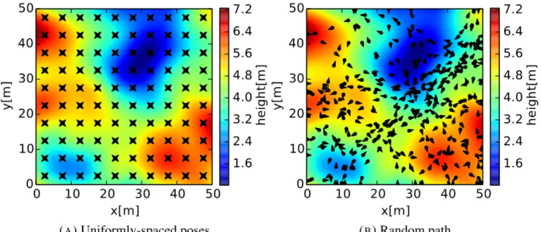
3.2 Example sets of sample poses used in tests with the GP model: on the left, a uniformly-spaced set, corresponding to a sweep pattern over the simulated terrain in 4 orientations; on the right, a
LIST OFFIGURES xi
random path where consecutive poses are separated from each other by a fixed-length segment
and a random turn angle. 57
3.3 Height map of the simulated terrain with executed paths for different settings of the UCB parameter λ(see Equation 3.11): Each candidate path is plotted with a dashed line, with the lowest-energy path found by the BO algorithm represented by a solid black line in each case. The optimum path, found by simulated annealing over the noise-free cost function, is also plotted in a solid white line. The robot’s start location(x0, y0) = (40,40)is marked
with a white cross (+) symbol. In all the cases, the robot’s initial heading isθ0 =−135o, i.e.
the robot is headed downwards along the diagonal. The goal point is also fixed, located at
(xf, yf) = (10,10). 58
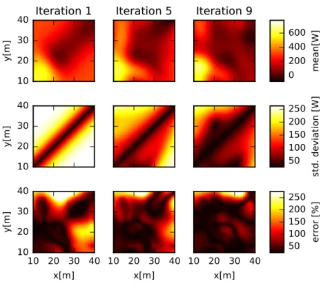
3.4 Evolution of the GP estimates for the robot’s power consumption on poses withθ=−135o, main direction of movement, after iterations 1, 5 and 9 for the test case in Figure 3.3b. The upper plots show the GP predictive mean for the power consumption level,µw(x). The middle
plots show the GP predictive variance (in terms of standard deviation, i.e. σw(x)). The lower plots show the relative error between the GP predictive mean and the computed ground-truth
costs, i.e.|1−µw(x)/w(x)|. 59
3.5 Averaged relative energy cost (%) between the current lowest-energy path found by each algorithm and the ground-truth optimum at each iteration. The error bars correspond to one standard deviation, computed over the re-runs of each algorithm. With only 5 iterations, the best paths found by the proposed BO planner are within 10% of the optimum. For these
comparisons,λ= 7was used (see Equation 3.11). 60
3.6 Examples of the lowest-energy paths found by each algorithm on the different terrains. 61 3.7 Robot used and partial view of the area where the field experiments were performed 63 3.8 Experimental results: (a) Aerial view of the experiments area overlaid with the paths
executed by the robot running the BO planner. (b) Paths planned by the algorithm, where the start positions are located on the left side of the plot, while the goal is on the right. (c) Predictions and measurements for the energy required to execute each path attempted by the
algorithm in the field experiments. 64
4.1 Restriction of the valid search space under track constraints: The plot on the left presents trajectory roll-outs for a robot car, starting at location(0,0), for a range of acceleration and
LIST OFFIGURES xii
shaded area in the left-side plot. The robot’s reward is either zero if it does not complete the track or its final speed, case it completes the track. The resulting reward surface is shown on the
right-hand side. 66
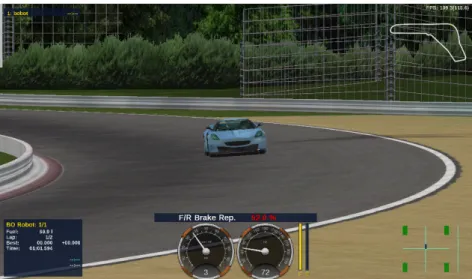
4.2 Screen-shot of the race car used in the experiments. 77
4.3 Detail of the effect of different lengths scales on the fitting of the initial policy for the same kernel placement. The recorded actions are shown in a dashed line. Shorter length scales allow sharper transition, but might compromise interpolation. Longer length scales yield smoother
curves, but might compromise flexibility 78
4.4 The race tracks for the experiments (Source:Speed Dreams) 79
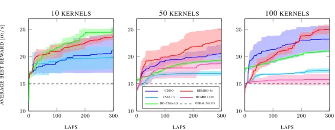
4.5 Performance vs. dimensionality onForza: More kernels allow for better policies, but make
the optimisation problem harder. Results were averaged over 4 trials. Shaded areas correspond
to 1 standard deviation. 80
4.6 Best policy obtained for trackForza 81
4.7 Performance vs. dimensionality onAllondaz: The plots show how the performance of each
algorithm is affected by the increase in dimensionality. Results were averaged over 4 trials.
Shaded areas correspond to 1 standard deviation. 82
5.1 At timet−1, the robot is estimated to be at some˜xt−1∼PtL−1with meanˆxLt−1. The robot is
then sent to target locationxt. However, due to uncertainty in the query execution, represented
byPxEt, the robot actually ends up at another location˜xt, whose belief distribution, according
to the localisation system, is represented byPtL. The robot’s true locations and true path are
indicated by the dashed lines. 88
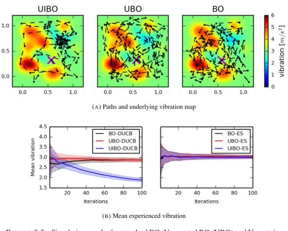
5.2 Effect of different values for the DUCB parameterβ usingζ = 1on UIBO’s performance. 93 5.3 Simulation results for standard BO, Unscented BO (UBO) and Uncertain-Inputs BO (UIBO)
methods for random functions modelling terrain-induced vibration. (a) presents the true paths taken by each BO method usingDUCBover the true vibration map in one of the test trials.
The markers along the paths indicate the locations where observations were taken. The big "X" mark (in magenta) indicates the starting location, which is the same for the three methods at each trial. The plots in (b) present performance results in terms of mean intensity of the experienced vibration. The results were averaged over 30 trials, each with different maps, and
LIST OFFIGURES xiii
5.4 Robot experiment details. (a) presents the experiments’ robotic platform. (b) compares different methods to measure vibration using an IMU:rawcorresponds to the raw vertical
acceleration readings (discounting gravity),meancorresponds to the mean value of the raw
measurements, considering a moving window of size 100, andRMS corresponds to the
root-mean-square value of the raw measurements in the same window. 96 5.5 Posterior mean of the GP model built by each BO method overlaid with their respective paths
according to locations estimated by an EKF fusing conventional GPS, IMU and odometry. In both cases, the robot started at the lower left corner of the map at the locations marked by a
white cross. 99
5.6 For visualisation purposes, posterior mean of a GP model built from the validation data taken
with RTK GPS high-precision location estimates. 99
6.1 Theory check: The plot shows the mean expected regret and its theoretical upper bound for each UCB algorithm. Results were averaged over 10 trials, each with randomly generated input
and output noise. 131
6.2 Mean expected regret for IGP-UCB, UEI, and uGP-UCB in the optimisation of functions in the same RKHS: in (a) the UCB confidence-bound parameterβtwas set according to the
theoretical results, while in (b), it was fixed atβt= 3for allt. The results were averaged over
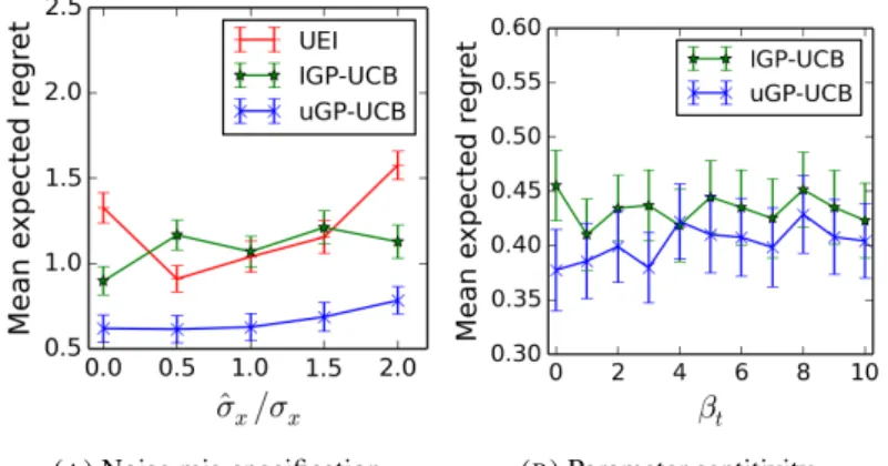
20 trials, and the shaded areas correspond to one standard deviation. 131 6.3 Robustness: (a) presents how each algorithm’s performance is affected by mis-specification
of the execution noise variance for the experiment with functions in the same RKHS, while (b) presents how the UCB methods performance varies under different settings forβtin the case
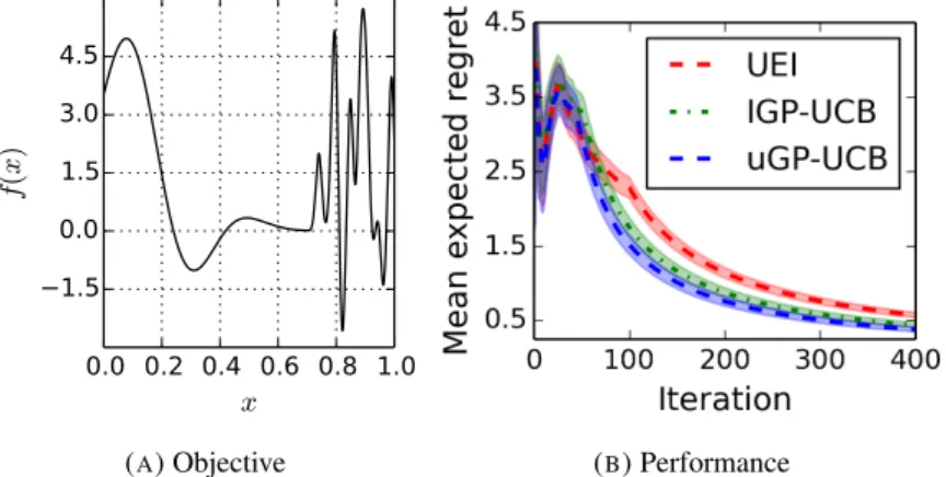
of the objective function in a different RKHS. In both cases, the mean expected regret shown is computed at the end of 200 iterations and averaged over 10 trials. 132 6.4 Performance results for objective function in different RKHS: (a) presents the objective
function and (b) the mean expected regret for each algorithm. Results were averaged over 10
trials. 133
6.5 Robotic exploration experiment: (a) presents the Broom’s barn data as distributed over the search space; (b) presents a typical execution error distribution as observed from one of the runs in the experiment; and (c) shows the performance of each BO approach, averaged over 4 runs. 134
List of Tables
3.1 Simulation settings 56
3.2 True energy and its estimates for the lowest-energy paths found by the BO path planner in
the test cases in Figure 3.3 58
3.3 Field experiment hyper-parameters 62
4.1 Average runtime (in seconds) onForza 82
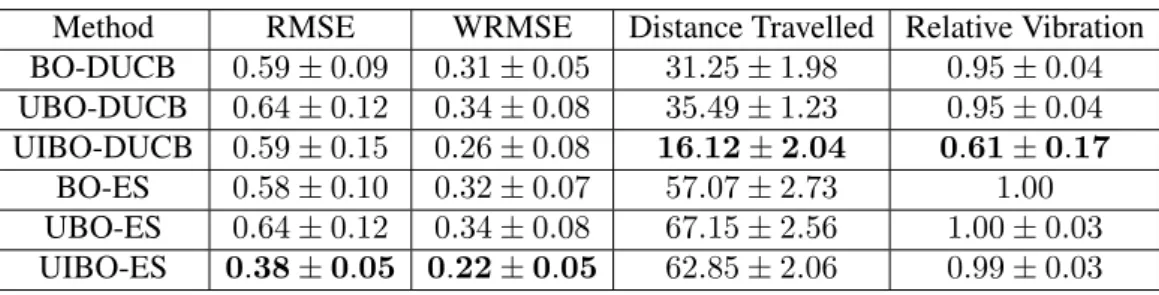
5.1 Simulation results: average performance comparisons for each BO approach under different metrics with the corresponding standard deviation (30 trials). 95 5.2 Field results: performance comparisons for each BO approach under different metrics. The
WRMSE was computed between the posterior mean of the final GP model at the locations in the validation dataset and the corresponding vibration measurements at those locations. 98
A.1 Notation 150
Nomenclature
Abbreviations
i.i.d. independent and identically distributed a.e. almost everywhere
a.s. almost surely
BO Bayesian optimisation
CDBO coordinate-descent Bayesian optimisation
CMA-ES Covariance Matrix Adaptation Evolution Strategy DUCB distance-penalised upper confidence bound EI expected improvement
GP Gaussian process
GPS Global Positioning System IMU inertial measurement unit RKHS reproducing kernel Hilbert space RMSE root mean square error
RTK real-time kinematics UCB upper confidence bound
WRMSE weighted root mean square error Basic fonts
a a scalar
a a vector
A a matrix
A a set
A a collection of sets, such as aσ-algebra (sigma-algebra) or a topology. A a functional or a measure
Matrix operations
[A]ij the element in thei’th row andj’th column ofA
AT transpose
NOMENCLATURE xvi
A−1 inverse tr(A) trace
|A| determinant
Basic operations
U \V the complement of setVinU hf, giF the inner product betweenf, g∈ F
lim sup
n→∞ an the limit superior of a real-valued sequence, i.e.lim supn→∞an:= limn→∞ supt≥nat
kfkF the norm off ∈ F
U the closure of the setU, i.e. the smallest closed set containingU.
x·y the dot product, i.e. the standard inner product in Euclidean vector spaces
f(U) The image of setU under the mappingf f−1(V) the pre-image of setVunder the mappingf
|F | the cardinality of a set, i.e. the number of elements in setF, or∞ifF is not finite |a| the absolute value ofa∈R
Special symbols
B(X) the Borelσ-algebra of a topological spaceX. CaseX =Rd,d∈N,Bd:=B(Rd).
Dn a dataset containingnentries
∅ the empty set
E expected value
µn(·) posterior mean function of a Gaussian process given a set ofnobservations
H a Hilbert space
Hk the reproducing kernel Hilbert space associated with a kernelk 1A(·) the indicator function of a setA
N the set of natural numbers, i.e. the positive integers,N={1,2,3, . . .}
N(ˆx,Σ) a normal distribution, i.e. a Gaussian probability measure, with meanˆxand covarianceΣ
P a probability measure
P{·} probability of an event involving random variables, e.g. for a random variableξdefined on
a probability space(X,A, P)and valued in(W,W),P{ξ∈ A}=P[ξ−1(A)],∀A ∈W.
R The field of real numbers, the real line
O big-O notation for the set of upper bounds valid up to a constant factor
σn2(·) posterior variance function of a Gaussian process given a set ofnobservations
CHAPTER 1
Introduction
1.1 Motivation
As civilisation advances, there has been an increasing need to understand our world and the countless processes that take place within it. Environmental issues, planetary exploration, social media behaviours and many other related problems have the common characteristic of requiring data to be modelled and understood (Figure 1.1). In this sense, robots have become powerful tools to actively collect data from their environments (Marchant and Ramos, 2012; Candela et al., 2017; Bessi and Ferrara, 2016). Machine learning algorithms (Murphy, 2012) running on robotic platforms have the opportunity to be supplied with data in a self-supervised approach, using the robot to label new data points. This kind of automation requires the development of algorithms to actively guide the robot through the data collection process.
Planning algorithms search for strategies to take a system from a non-ideal initial state to a better, so called, goal state (LaValle, 2006). When applied to robotic systems, planners can guide the robot through the environment in order to accomplish a pre-defined task, such as learning an environmental model. Information from observed data allows us to validate and update theoretical models to explain different kinds of physical environments and their dynamics. At the same time, models aid the planning algorithm in guiding the robot, either to avoid hazards, such as obstacles and areas difficult to traverse, or to indicate areas in the model where more data is needed. However, each robot is limited by its sensors.
Sensors allow robots to perceive the world around them, but each sensor is subject to limitations. Cam-eras and laser ranging sensors cannot see through obstacles. Global positioning systems are subject to atmospheric interferences, multi-path reflections and satellite visibility. Orientation sensors, such as in-ertial measurement units, provide estimates that drift over time. All of these add uncertainty to models learnt from sensor data.
1.1 MOTIVATION 2
(A) Planetary exploration (B) Air pollution
(C) Social media
FIGURE 1.1: Modern issues demanding increasing amounts of data: (a) Spacecrafts
and robots have been sent to explore other planets in our solar system (Courtesy from NASA/JPL). (b) Increasing demands for energy and manufactured goods have been causing environmental issues, such as air pollution (Courtesy from Pexels.com). (c)
Social media behaviours have interested both marketing companies and governments (Courtesy fromPexels.com).
Besides uncertainty from the sensors, planning algorithms usually assume that a pre-defined cost map is available to evaluate the feasibility of certain actions with a robot (Zucker et al., 2013). When traversing unknown environments, however, information about motion feasibility, as provided by traversability metrics (Martin et al., 2013), geometric maps and dynamical models (Liniger et al., 2015), can only be acquired online, breaking classical assumptions.
This thesis is motivated by planning problems where limited prior information leads to uncertainty about the outcomes of decisions. The motivation is mainly based on robotics problems, which present challenges that can illustrate well this thesis’ concerns. However, the techniques are derived in a general approach, so that they can also be applied to areas outside of robotics.
1.2 BAYESIAN OPTIMISATION AS A FRAMEWORK FOR PLANNING UNDER UNCERTAINTY 3
1.2 Bayesian optimisation as a framework for planning under uncertainty
Planning actions for a robot can be formulated as an optimisation problem (Marchant and Ramos, 2012; Zucker et al., 2013; Marinho et al., 2016; Mukadam et al., 2017). In this case, one acts in order to optimise an objective function, which encodes goals and costs. In the case of motion planning, costs can usually be expressed as convex objectives, so that gradient-based approaches are well-suited (Zucker et al., 2013). However, other problems offer non-convex objectives. In this case, global optimisation is desired, such as finding:
x∗ ∈argmax
x∈S
f(x), (1.1)
whereS ⊂Rdis a compact search space where the algorithm can choose its actions, or queries,xfrom, andf is the objective function. In practice, the objective may represent an environmental process, a
terrain model, the performance of a given policy, or other objects of interest. Actions can correspond to spatial locations in an environmental process, parameters of a control policy, trajectories, etc. An optimisation algorithm can then use a robot to evaluate each action and find an optimal one.
For an arbitrary problem, the objective function is usually not known in closed form. Traditional op-timisation methods that require gradients are therefore not applicable. In addition, evaluations of the objective function with a robot can be costly and noisy due to limitations on the robot, such as energy supply and sensor imperfections. Techniques that do not depend on gradients, such as evolutionary methods (Arnold and Hansen, 2010), and Lipschitz optimisation (Malherbe and Vayatis, 2017), usually require a large amount of function evaluations or assume noiseless observations.
Bayesian optimisation (BO) offers a principled approach to solve optimisation problems where objective function evaluations are noisy and expensive (Brochu et al., 2010; Shahriari et al., 2016). BO algorithms have found success in a variety of applications, such as tuning parameters for machine learning al-gorithms (Snoek et al., 2012), robotic environmental monitoring (Marchant and Ramos, 2012), policy search (Wilson et al., 2014), computational biology (Ulmasov et al., 2016), etc. Objectives can be con-sidered as partially-observable functions of the algorithm’s queries, i.e. the output is only observable through noisy samples. A BO algorithm then learns a probabilistic model of the objective function by observing the outcomes of its own actions. The model is combined with selection criteria to choose which actions should be tried next by the algorithm at each stage of the process. More details about the BO framework will be presented in Chapter 2.
1.4 CONTRIBUTIONS 4
1.3 Problem statement
Despite its success, many open problems are still present when applying Bayesian optimisation to robot-ics, a few of which this thesis considers. Firstly, BO has been applied to optimise continuous informative paths over environmental processes (Marchant and Ramos, 2014). Then it might be possible to apply BO as a method to optimise paths over unknown terrains that robots need to traverse. Secondly, deal-ing with the optimisation of paths and policies (Wilson et al., 2014) may also lead to high-dimensional parameter spaces, which leads to problems in BO that have only recently been explored (Chen et al., 2012; Wang et al., 2013; Kandasamy et al., 2015; Wang et al., 2018a). Lastly, a common assumption in BO approaches is that queries are executed precisely at where they were intended to be. When using a robot to execute queries, that assumption typically does not hold, and very few BO methods have been recently proposed to address this issue (Nogueira et al., 2016; Beland and Nair, 2017). In addition, esti-mates of the query location can be provided as probability distributions by localisation systems (Thrun et al., 2006). BO algorithms may be able to use probability distributions, instead of point estimates, to learn models of an objective function.
In a general, high-level description, this thesis addresses the problem of:how to select actions to perform with a robot in order to optimise a partially-observable objective? Partial observability means that the
outcomes of the robot’s actions can only be observed through samples subject to noise. It is also assumed that evaluations are costly and limited by a given budget.
1.4 Contributions
This thesis is composed of four contributing chapters, whose main contributions are summarised below.
1.4.1 Finding feasible paths
Chapter 3 addresses the possibility of using BO methods to learn feasible paths for a robot to navigate through unknown terrain. The chapter presents a BO algorithm to select energy-efficient paths between given start and goal locations while learning a model of the robot’s power consumption over the terrain. The model is based on Gaussian process (GP) regression (Rasmussen and Williams, 2006), and paths are formulated as parametric curves. Experiments evaluate the approach both in simulation and with a physical robot.
1.4 CONTRIBUTIONS 5
1.4.2 BO in high-dimensional search spaces
Optimising paths and control policies leads to high-dimensional search spaces. Chapter 4 then proposes a BO method to optimise functions of many parameters by combining BO with coordinate-descent schemes. The method is applied to the problem of learning control policies for a robot race car with the goal of minimising its lapping time. The algorithm has no prior information about the track nor the robot’s dynamical model, just an initial sub-optimal policy example. Policies are parameterised as functions in a reproducing kernel Hilbert space (RKHS) (Schölkopf and Smola, 2002). Experiments demonstrate the performance of the algorithm against other optimisation methods in a simulated racing environment.
1.4.3 Planning under localisation uncertainty
When dealing with physical robots, localisation uncertainty may corrupt models and mislead algorithms guiding the robot. The traditional approach is to either use mean estimates or to assume that the robot is following its intended trajectory. Chapter 5 investigates problems where location distributions provided by localisation systems (Thrun et al., 2006), instead of point estimates, can be used as inputs to models of the robot’s environment. The chapter proposes a method using a Gaussian process model that takes probability distributions as inputs as a prior for BO. The proposed method also applies heuristics that consider the distance between the sampling locations when deciding where to send the robot next. An application is given to the problem of learning terrain roughness models while safely navigating the robot, and it is evaluated both in simulation and in an experiment with a physical robot.
1.4.4 Optimisation under uncertain inputs
The investigation in Chapter 5 opens up the question of whether a Bayesian optimisation algorithm can maintain theoretical convergence guarantees in problems involving uncertain inputs. Chapter 6 then presents a method for BO under uncertain inputs and theoretical guarantees for this method. The chapter also presents under which assumptions a conventional BO algorithm (Chowdhury and Gopalan, 2017) may converge despite the presence of noisy inputs. Experiments in simulation complement the results by evaluating the performance of the different BO approaches to input noise in a variety of scenarios.
1.5 OUTLINE 6
1.5 Outline
After this introduction, this thesis’ main components are a background chapter, followed by four con-tributing chapters, and a conclusion, which are outlined below.
Chapter 2 presents the theoretical background necessary to understand the main contributions of this the-sis. Bayesian optimisation and Gaussian processes are formally introduced. The chapter also presents reproducing kernel Hilbert spaces, present in chapters 4 and 6, and other background necessary to un-derstand the results in Chapter 6.
The four contributing chapters (3 through 6) follow the same basic structure. After a motivating intro-duction, each chapter describes related work, methodology and experiments. Chapter 3 presents the first contribution of this thesis: a method to find energy-efficient paths over unknown terrains. As a second contribution, Chapter 4 presents a BO method for policy-search problems involving high-dimensional parameter spaces. Chapter 5 addresses the problem of planning under localisation uncertainty, providing a method to learn terrain roughness models while safely navigating a mobile robot. Based on the inves-tigation in the previous chapter, as a final contribution, Chapter 6 provides a method with theoretical guarantees to solve more general optimisation problems under uncertain inputs.
The thesis closes in Chapter 7 with a review of the contributions and directions for future research. In addition, Appendix A, at the end of the thesis, presents the derivation of proofs for auxiliary theoretical results, such as lemmas and propositions, which were presented in Chapter 6.
CHAPTER 2
Background
This chapter presents a review of concepts that form the basis for the methods this thesis proposes. Most of the problems faced by this work deal with variables assumed to be uncertain. In this case, a logical choice of approach is to apply probabilistic models and Bayesian reasoning. To form a basis for this approach, the chapter begins by reviewing some of the basic concepts of supervised learning in the Bayesian setting (Section 2.1). The focus is on regression models. In particular, Gaussian process (GP) regression (Section 2.2) is present throughout this thesis. Bayesian optimisation with GP priors is introduced in Section 2.3. GPs are also closely related to the topic of reproducing kernel Hilbert spaces (Section 2.4), which have their own variety of applications. The chapter also presents a review on some of the basics of topology (Section 2.5) and measure theory (Section 2.6), which play a role in most of the theoretical results in Chapter 6. Lastly, the chapter closes in Section 2.2.4 with a discussion on GP models accounting for noisy inputs. At the end of the chapter, a brief summary of the topics with their connections to the rest of the thesis and a few final bibliographical remarks are provided.
2.1 Bayesian learning
Let us begin by considering the case of supervised learning (Murphy, 2012). Consider a datasetD =
{(xi, yi)}ni=1composed ofninput-output pairs(xi, yi). Our task is to learn a functionf mapping each
inputxi to the corresponding outputyi, so that we can predict the function value at unobserved inputs.
We can be general about the inputs, assuming they are d-dimensional vectors from a set X ⊂ Rd.
The outputs, we will assume that they are real-valued scalars, y ∈ R. In addition, we consider that
observations are corrupted by noise, so that:
yi=f(xi) +νi, i= 1, . . . , n , (2.1) 7
2.1 BAYESIAN LEARNING 8
whereνiis independent and identically distributed (i.i.d.) random noise drawn from a given probability
distribution. In general, we will consider that the noise follows a zero-mean Gaussian distribution with varianceσν2, i.e.νi∼N(0, σ2ν).
To solve the problem above, we consider thatfcomes from a known hypothesis spaceHand try to find
thef ∈ Hthat best explains the data inD. In the case of linear regression, for example, we assume that:
f(x) =wTx, (2.2)
where the vectorwcomposes the set of parameters of our model. The hypothesis space in this case is simplyH ={f :X → R |f(x) =wTx,w∈
Rd}. We can generalise that to the case of non-linear
models by adopting a set of non-linear basis functionsφi :X →R, i∈ {1, . . . , q},q ∈N, and having:
f(x) =wTφ(x), (2.3)
whereφ(x) := [φ1(x), . . . , φq(x)]T. In this case, the hypothesis space is given byH={f :X → R| f(x) =wTφ(x),w∈
Rq}.
Given a set of parameterised functions, the task is to find the parameterswthat best explain the data we observe. In general, this problem is formulated as minimising a data-dependent loss function over the hypothesis space, picking the w that best fits to it. However, there are a few drawbacks to that approach. The main issue here is that it becomes difficult to infer how confident the model is about its predictions given a limited amount of noise-corrupted data. Having models whose degree of uncertainty is quantifiable allows us to take such uncertainty into account when making decisions.
Bayesian learning quantifies model uncertainty by placing a belief distribution over the model we are trying to learn and updating that belief according to the observed data. Predictions are then performed via inference over the posterior distribution of the model conditioned on the data. By Bayes’ rule, in the parametric case, the density of this posterior belief distribution at a givenwis:
p(w|D) = p(w,D)
p(D) =
p(D|w)p(w)
p(D) , (2.4)
wherep(D|w)corresponds to the likelihood of the parameters,p(w)is the prior, andp(D)is called the evidence or the marginal likelihood (MacKay, 2003, Sec. 2.3). As a probability distribution, we can use the posteriorp(w|D) to assess how probable each choice ofwis to be the correct one. The posterior probabilityp(w|D)then encodes the model’s confidence.
2.2 GAUSSIAN PROCESSES 9
In the case of Bayesian linear regression (Murphy, 2012, Sec. 7.6), we can assume a Gaussian prior over the parameters vector,w∼N(0,Σw). Assuming i.i.d. zero-mean Gaussian noiseνi ∼N(0, σν2), the
joint distribution between the data and the parametersp(w,D)is then given by:
w y ∼N 0, Σw ΣwΦT ΦΣw ΦΣwΦT+σν2I , (2.5)
wherey= [y1, . . . , yn]TandΦis an-by-qmatrix with elementsΦij =φj(xi). Conditioning the joint
(Equation 2.5) on the dataD, we get the posterior distribution (Equation 2.4) as:
w|D ∼N(ΣwΦTΣ−D1y, Σw−ΣwΦTΣ−D1ΦΣw), (2.6)
whereΣD:=ΦΣwΦT+σν2I. Now, given a query pointx∗∈ X, the value off(x∗)follows:
f(x∗)|D ∼N(φT∗ΣwΦTΣ−D1y, φT∗Σwφ∗−φT∗ΣwΦTΣ−D1ΦΣwφ∗), (2.7)
whereφ∗:=φ(x∗). The mean of the above distribution is our most likely prediction forf(x∗), and the variance quantifies the level of uncertainty about that prediction.
As discussed in Rasmussen and Williams (2006, Sec. 2.1.2), φ(x) maps thed-dimensional vectorx into aq-dimensional feature space. These maps appear in the predictive distribution (Equation 2.7) in
the general form of(x,x0) 7→ φ(x)TΣ
wφ(x0). The latter defines a positive-definite kernel or
covari-ance function k(x,x0) = φ(x)TΣ
wφ(x0). Kernels allow abstracting feature maps to even
infinite-dimensional feature spaces without having to deal with the elements of such spaces directly, leading to non-parametric methods. Kernel methods form an essential part of this thesis and will be further reviewed in the following sections.
The next two sections present kernel methods for Bayesian learning. Section 2.2 introduces Gaussian process regression, which arises as a natural extension of the parametric framework in Bayesian linear regression to the non-parametric setting. Section 2.4 presents reproducing kernel Hilbert spaces, which connects kernel methods to functional analysis through the framework of Hilbert spaces.
2.2 Gaussian processes
Gaussian process (GP) models (Rasmussen and Williams, 2006) provide a non-parametric framework for Bayesian inference over function spaces. Non-parametric here means that a model’s parameters are
2.2 GAUSSIAN PROCESSES 10
not explicitly taken into account, but are inferred from the data, instead. This characteristic allows a model to be updated by simply adding a new data point without the need for retraining. As probabilistic models, GP predictions are probability distributions. In particular, a GP directly models a distribution over a space of functions, enabling Bayesian reasoning in that space.
By definition, a Gaussian process is a stochastic process (Bauer, 1981), i.e. a collection of random variables, whose finite sub-collections follow a joint Gaussian distribution (Rasmussen and Williams, 2006, Def. 2.1). Stochastic processes can also be interpreted as random functions (Berlinet and Thomas-Agnan, 2004; Rasmussen and Williams, 2006), which is the approach taken here to describe GPs.
Analogously to conventional multivariate Gaussian distributions, which are specified by a mean vector and a covariance matrix, a GP is completely specified by amean function and acovariance function.
Let’s say we want to model a functionf : X →R, considering an arbitrary domainX ⊂ Rd. A GP
model with mean functionm : X → R and positive-definite covariance functionk : X × X → R
places a prior on f so that, for any finite collection of query points {xi}ni=1 ⊂ X, the vectorfn =
[f(x1), . . . , f(xn)]Tis distributed according to a Gaussian:
fn∼N(mn,Kn), (2.8)
wheremn:= [m(x1), . . . , m(xn)]Tand[Kn]ij =k(xi,xj).
Now assume we are given a set of observationsDn ={(xi, yi)}ni=1, whereyi =f(xi) +νi, andνi ∼ N(0, σν2). Suppose we want to infer the value of the function at a given query pointx∗∈ X. According
to the Gaussian process model, the vector of observationsyn:= [y1, . . . , yn]Tand the function value at
the query locationf(x∗)are joint normally distributed:
yn f(x∗) ∼N mn m(x∗) , Kn+σν2I kn(x∗) kn(x∗)T k(x∗,x∗) . (2.9)
wherekn(x∗) := [k(x1,x∗), . . . , k(xn,x)]T. Conditioning the joint distribution in Equation 2.9 on the
observations, we have that:
2.2 GAUSSIAN PROCESSES 11
where:
µn(x∗) =m(x∗) +kn(x∗)T(Kn+σν2I)−1(yn−mn), (2.11) kn(x,x0) =k(x,x0)−kn(x)T(Kn+σ2νI)−1kn(x0), (2.12)
σn2(x∗) =kn(x∗,x∗). (2.13)
This predictive distribution allows us to infer function values at unobserved locations. Also note thatkn
in Equation 2.12 defines a valid covariance function, so thatGP(µn, kn) is a Gaussian process, often
referred to as the posterior GP (Srinivas et al., 2010).
2.2.1 Covariance functions
The GP covariance function determines how the values of random functions at different query points co-vary, i.e.:
Covf∼GP(m,k)(f(x), f(x0)) =k(x,x0), (2.14)
whereGP(m, k) represents a GP prior with mean m and covariancek. To define a valid covariance
function, k : X × X → R needs to be positive definite, i.e. for all n ∈ N, α1, . . . , αn ∈ R and
{xi}ni=1⊂ X,ksatisfies: n X i=1 n X j=1 αiαjk(xi,xj)≥0. (2.15)
In particular, if equality only holds forα1 =· · ·=αn= 0,kis called strictly positive definite1.
Considering the Bayesian linear regression example in Equation 2.7, we have that:
k(x,x0) =φ(x)TΣwφ(x0),∀x,x0 ∈ X , (2.16)
defines a positive-definite covariance function. If we rewrite Equation 2.7 in terms of k, we obtain
exactly the GP predictive equations (Equation 2.11 and Equation 2.13) for the zero-mean case. Hence, a Bayesian linear regression model with Gaussian prior on the weights can be interpreted as a particular type of GP model.
1Note that this definition can be confused with the case of matrices. Some authors actually refer to what was defined as a positive-definite kernel in Equation 2.15 as positivesemi-definite(Rasmussen and Williams, 2006). That terminology only calls positive definite the kernels that were defined asstrictlypositive definite in the description above. This thesis, instead, adopts the terminology above, since most of the theory holds if the kernels are simply positive definite, as defined.
2.2 GAUSSIAN PROCESSES 12
The GP literature is filled with several other types of covariance functions for GP models. The remainder of this section presents a few covariance functions used throughout the work in this thesis. For more examples, the reader is referred to Rasmussen and Williams (2006, Ch. 4).
Linear covariance functions: One of the simplest cases is given by thelinearcovariance function: k(x,x0) =xTAx0+b ,∀x,x0 ∈Rd (2.17)
whereAis any positive-definite matrix andb ≥0. This covariance function allows us to model linear functions of the formf(x) =aTx+c, wherea∈
Rdandc∈R.
Translation-invariant covariance functions: Another set of covariance functions is given by those with a translational-invariance property, i.e. k(x,x0) = k(x−x0,0). For instance, many types of
covariance functions can be defined as a radial function in terms of some distance metricρbetween the
data points, i.e.:
k(x,x0) =k(ρ(x,x0)). (2.18)
Translation invariance leads to astationaryGaussian process, i.e. the distribution of the process is not
affected by a translation of the input space (Ledoux and Talagrand, 1991, p. 368). Hence, translation-invariant covariance functions are also referred to asstationary.
Stationary covariance functions: One of the most popular stationary covariance functions is the
squared exponential, which is commonly given by:
k(x,x0) =σf2exp −1 2ρ 2 L(x,x0) , (2.19)
whereσf2 is called the signal variance parameter, and:
ρL(x,x0) := q
(x−x0)TL−1(x−x0) (2.20)
is a common distance function for vectorial inputs, whereLis a positive-definite matrix used for scaling. For being infinitely many times differentiable with respect to its inputs (Rasmussen and Williams, 2006), the squared exponential covariance function models very smooth functions with a GP. However, in most applications, such a level of smoothness is unrealistic. Therefore, another popular family of covariance functions is theMatérnclass, which provides a controllable smoothness parameterνin its construction
2.2 GAUSSIAN PROCESSES 13
non-negative integer, the Matérn covariance functions are given by:
k(x,x0) =σ2fexp −√2νρL(x,x0) p! (2p)! p X i=0 (p+i)! i!(p−i)! √ 8νρL(x,x0) p−i , (2.21)
In the later chapters, we will specially make use of Matérn covariance functions with ν = {12,32,52},
commonly referring to them by the numerator (e.g. Matérn 1 refers toν = 1/2).
Hyper-parameters: The parameters of the covariance function, the noise model and the mean func-tion of the GP model are referred to as the hyper-parameters of the model. In the case of the stafunc-tionary covariance functions presented above, the noise model varianceσ2ν, the signal varianceσ2f andL com-pose the set of hyper-parameters for a stationary zero-mean GP model. CommonlyL is chosen as a diagonal matrix with[L]ii =`2i, `i >0, i∈ {1, . . . , d}. Each`i is called alength-scale, as it controls
the scaling of thei’th coordinate in the input space. The larger`i is, the lower is the sensitivity of the
covariance function to changes in thei’th coordinate. In the special case whenL=`2I, having a single
length-scale, the covariance function is said to beisotropic, since it varies equally across all directions.
2.2.2 Hyper-parameter learning
The hyper-parameters of a GP play an important role in determining the capability of a model to explain real data. Ideally one should know the hyper-parameters of a GP model in advance, as they are part of the prior over the function space being modelled. However, that is rarely the case in practice.
The machine learning literature provides a few approaches to handle unknown hyper-parameters by learning them from data (Rasmussen and Williams, 2006; Snoek et al., 2012; Wang et al., 2018b; Berkenkamp et al., 2019). The most popular approaches are based on type-II maximum likelihood (MLE) or maximum a posteriori (MAP) estimation (Rasmussen and Williams, 2006). Given a dataset withnobservationsDn={(xi, yi)}ni=1, the marginal likelihoodp(Dn|θ)basically determines how well
GP hyper-parametersθ explain the observed dataDn by marginalisingfn out of the joint probability
densityp(yn,fn|θ)given by Equation 2.9. As a result, we obtain:
logp(Dn|θ) = logp(yn|θ) =−1 2(yn−m θ n)T(Kθn+σ2νI)−1(yn−mn)− 1 2log|K θ n+σν2I|− n 2 log 2π , (2.22) where|Kθn+σν2I|represents the determinant of the matrixKθn+σ2νI, and the superscripts withθdenote
2.2 GAUSSIAN PROCESSES 14
Equation 2.22 can be maximised with respect to the hyper-parameters by gradient-based methods, when derivatives of the covariance functions with respect to the hyper-parameters are available, or by derivative-free methods, otherwise. In the works presented by this thesis, in particular, we applied local optimisation algorithms, such as the derivative-freeConstrained Optimization by Linear Approximations
(COBYLA) (Powell, 1998) and the sub-gradient-based RPROP algorithm (Riedmiller and Braun, 1993), depending on whether or not derivatives of the covariance function with respect to its hyper-parameters were available.
Optimising Equation 2.22 with respect to hyper-parameters within a bounded search space is equivalent to placing a uniform priorp(θ)over the hyper-parameters, so that MLE is equivalent to a MAP solution in this case. To perform MAP estimation with more informative priors (see Lizotte, 2008, e.g.), one can addlogp(θ)to Equation 2.22, which then acts as a regularisation term in the optimisation process.
2.2.3 Computational complexity and sparse approximations
One of main sources of computational complexity in traditional GP approaches is the inversion of the kernel matrixKn (see Equation 2.9). This operation scales asO(n3) with the number of data points.
Although not applied in this thesis, the GP literature is filled with approximation methods to address this issue. One could use, for example, sparse approximations based on Fourier features (Rahimi and Recht, 2007), which lead to sparse spectrum Gaussian processes (Lázaro-Gredilla et al., 2010). Sparse spectrum models can achieve low computational costO(nq2), whereqis the number of Fourier features,
when using incremental updates (Gijsberts and Metta, 2013), making them suitable for online learning applications, as in Bayesian optimisation (Mutný and Krause, 2018). Another popular approach is to use sparse GP models based on variational inference approaches (Hensman et al., 2013), which usually require batch data. Adapting these models to online learning for Bayesian optimisation has also been done (Mcintire et al., 2016). However, such approach leads to costly operations in the updates of the variational parameters.
2.2.4 GP models accounting for input noise
Consider that measurement and execution noise affect the evaluation of a functionf :X → R, where X ⊂Rd. In this case, given a desired query inputx∗ ∈ X, the actual location where the observation is
collected at, i.e. ˜x∗|x∗ ∼P∗, is not directly observable. Assuming thatf ∼GP(m, k), the distribution
2.2 GAUSSIAN PROCESSES 15 p(f(x)) 0.5 0.0 0.5 1.0 1.5 f(x) 6 4 2 0 2 4 6 x p(x)
FIGURE 2.1: The effects of input noise on queries to a non-linear function. The
func-tion in the middle plot has been sampled from a squared-exponential GP model. The bottom plot presents a Gaussian query distribution. The top-left plot shows the distribu-tion of output values. As seen, the resulting distribudistribu-tion of funcdistribu-tion values is no longer Gaussian due to the function’s non-linearity.
posterior (Equation 2.11 and Equation 2.13). Therefore, the resulting stochastic process that represents
f under noisy inputs is no longer a Gaussian process and lacks an analytic formulation (Girard, 2004;
Damianou et al., 2016). Figure 2.1 presents an example where Gaussian noise affects the query of a function sampled from a GP.
The expected Gaussian process
In the machine learning literature, different methods have been proposed to learn Gaussian process models over functions with noisy inputs (Girard, 2004; Mchutchon and Rasmussen, 2011; Dallaire et al., 2011; Damianou et al., 2016). As demonstrated by Girard (2004), one can formulate a Gaussian process approximation forfby using the iterated mean and covariance of the resulting stochastic process under
the influence of input noise. In particular, in the case of a constant deterministic mean functionm(x) =
m0, ∀x∈ X, the mean and the covariance of this noisy process are given by:
E˜x[Ef[f(˜x)]] =m0 (2.23)
Covf,˜x,˜x0[f(˜x), f(˜x0)] =E ˜
2.2 GAUSSIAN PROCESSES 16
Therefore, for a set of independent random variables{˜xi}ni=1with corresponding distributions{Pi}ni=1,
we can define theexpectedcovariance function (Dallaire et al., 2011) as:
ˆ k(Pi, Pj) :=E[k(˜xi,x˜j)] = E[k(˜xi,x˜j)] = R X R X k(x,x0) dPi(x) dPj(x0), i6=j E[k(˜xi,x˜i)] = R Xk(x,x) dPi(x), i=j . (2.25)
Notice that, when˜xi and˜xj represent the same random variable, the above equation becomes a single
expectation under the same input distribution.
Depending on the type of input distributions and the original kernel for deterministic inputsk,
approx-imate and analytical solutions for Equation 2.25 are available in the literature (Girard, 2004; Dallaire et al., 2011; O’Callaghan and Ramos, 2012). An example is the squared exponential kernel in Equa-tion 2.19. In this case, if the input distribuEqua-tions are Gaussian, the resulting covariance funcEqua-tion, according to Dallaire et al. (2011), is given by:
ˆ
k(N(ˆxi,Σi), N(ˆxj,Σj)) =
σ2fexp −12(ˆxi−ˆxj)T(L+Σi+Σj)−1(ˆxi−ˆxj)
|I+L−1(Σi+Σj)(1−δij)|1/2
, (2.26)
whereσf2andLare the same hyper-parameters as described for the standard squared exponential kernel in Equation 2.19 andδij denotes the Kronecker delta. As seen, though probability measures are abstract
objects, ˆkcan be formulated as a function of the parameters of the input distributions, making them tractable, in practice.
The posterior of the stochastic process representingf ∼ GP(m, k)under input noise is not Gaussian due to the non-linear form of Equation 2.11 and Equation 2.13 with respect to the queryxand the data pointsxi. Yet one can obtain a suitable approximation for the originalf in the noisy input setting by
doing inference over a GP with meanm and covariance functionˆk, as defined in Equation 2.25. Such
model is referred to as theexpected Gaussian processmodel by Dallaire et al. (2011).
Despite the name, notice that theexpectedGP model does not truly represent the expected process. The
true expected GP would require to compute expectations of the posterior mean and posterior variance with respect to the distributions of both the query point and the data points, which can become easily intractable. Following the terminology adopted by Dallaire et al. (2011), this thesis refers toexpected Gaussian processas simply the model obtained by using the expected covariance function, as defined in
2.3 BAYESIAN OPTIMISATION 17
GP predictions under uncertain inputs
Equation 2.25 defines a covariance function over the setP of all probability measures onX. A GP
model with zero mean and covariance functionˆk:P × P →Rplaces a prior over the space composed of functionsgˆ: P →R. Inference can then be done similarly to the way it is done with conventional
GP models (Section 2.2). Given a set of observationsDn = {(Pi, yi)}i=1n , whereyi = ˆg(Pi) +νiand Pi∈ P, under the assumption thatνi ∼N(0, σν2), we have that the GP posterior meanµˆnand variance
ˆ σn2, at a givenP∗∈ P, are: ˆ µn(P∗) =ˆkn(P∗)T(Kˆn+σν2I)−1yn, (2.27) ˆ σ2n(P∗) = ˆk(P∗, P∗)−kˆn(P∗)T(Kˆn+σ2νI)−1ˆkn(P∗), (2.28) withˆkn(P
∗) := [ˆk(P∗, P1), . . . ,kˆ(P∗, Pn)]Tand[Kˆn]ij = ˆk(Pi, Pj). If˜x∗|x∗ ∼P∗, the expected GP
formulation approximates the posterior overf(˜x∗)as:
p(f(˜x∗)|x∗,Dn)≈N(ˆµn(P∗),ˆσn2(P∗)). (2.29)
This model is applied in Chapter 5 as a prior for a Bayesian optimisation algorithm to safely navigate a mobile robot over rough terrain under localisation uncertainty.
2.3 Bayesian optimisation
Consider the problem of searching for the global optimum of a function f : Rd → R within a given
compact search spaceS ⊂Rd, i.e. finding2:
x∗ = argmax
x∈S
f(x). (2.30)
Assume thatfis unknown to us and we only have access to noisy observations of its outputy=f(x)+ν
withν ∼N(0, σ2
ν). In addition, we are only allowed to sample the function up tontimes.
Bayesian optimisation (Brochu et al., 2010) assumes thatf(x)is a random variable and applies a prob-abilistic model as a prior overf. Using a Gaussian process model, BO encodes prior assumptions about f via the meanmand the covariance functionkof the GP.
2argmax corresponds to the set of arguments that maximise a function, which may contain multiple elements. The use of x∗= argmaxx∈Sf(x), instead ofx
∗
∈argmaxx∈Sf(x), indicates the assumption that there is only onex ∗
∈ Sfor which
2.3 BAYESIAN OPTIMISATION 18
(A) Objective (B) Observations (C) GP prior
(D) Acquisition function (E) Updated GP (F) Updated acquisi-tion funcacquisi-tion
FIGURE 2.2: Illustration of the BO process: Consider an unknown objective function f and its global optimumx∗ in a given search spaceS (a). Only noisy observations
(b) are available. At each iterationt, BO fits a GP model overf with the current set of
observations (c). Then BO maximises an acquisition function, which takes into account the GP model, to select the next query point xt (d). The function is sampled at xt,
providing BO with a new observation to update the GP with (e). The algorithm then proceeds by selecting a new query pointxt+1with the updated acquisition function (f).
Rather than directly searching overf, BO uses anacquisition functionh(x)as a guide to sequentially select input locations at which to observef. The acquisition function uses the information provided by
the GP prior and the observations off to estimate an utility value for samplingf at a givenx. So at
each iterationt, BO queries the objective functionf at the location of highest utility according to the
acquisition function, considering the data observed so farDt−1, which is given by:
xt= argmax x∈S
h(x|Dt−1). (2.31)
After observing f at xt, BO updates the GP observations dataset with the new pair (xt, yt), which
improves the belief about f. Then the algorithm proceeds to the next iteration, choosing an xt+1.
The BO loop runs until a stopping criterion is satisfied, which is usually defined by a total number of iterations,n. At the end of this process, BO obtains a model that approximates the objective function f|Dn∼GP(µn, σn2)and an estimate of the optimum locationx∗, given by the best sample in the dataset.
2.3 BAYESIAN OPTIMISATION 19
Algorithm 1:Bayesian optimisation Input:
S: search space
n: total number of iterations
1 fort∈ {1, . . . , n}do 2 xt= argmax x∈S h(x|Dt−1) 3 yt←Samplef(xt) 4 Dt=Dt−1∪ {(xt, yt)} 5 t∗= argmax t∈{1,...,n} µn(xt) Result:µn, σ2n,xt∗ 2.3.1 Regret analysis
To derive theoretical guarantees for BO algorithms, a quantity that plays an important role in the theory isregret. BO can be classified as a multi-armed bandits algorithm (Srinivas et al., 2012). In the bandits
literature (Arora et al., 2012), regret basically measures how good the algorithm’s actions were when compared to optimal choices. The latter corresponds to the decision that an algorithm with perfect knowledge about the objective would make. There are many types of regret definitions available in the bandits literature (Arora et al., 2012). However, the work in this thesis is mainly concerned withinstant regretandcumulative regret, which are defined as follows.
Consider a continuous functionf : S → Rdefined over a compact set S. At each roundt ∈ N, a
maximisation algorithm overfselects query pointsxt∈ S. The instant regret suffered by the algorithm
at roundtis defined as:
rt:= max
x∈S f(x)−f(xt), (2.32)
while the cumulative regret afternrounds is defined as:
Rn:= n X
t=1
rt. (2.33)
A desirable characteristic of an optimisation algorithm is to have no regret, at least asymptotically, i.e. lim
n→∞mint≤nrt = 0. With vanishing regret, asn→ ∞, we have thatmaxt≤nf(xt)→ maxx∈Sf(x).
From the definitions above, one can see that theoretical results providing upper bounds for the cumulative regret of an optimisation algorithm also bound the instant regret, sincemint≤nrt≤ Rnn. Asymptotically
vanishing regret then happens whenever the cumulative regret grows sub-linearly, yielding lim
n→∞ Rn
2.3 BAYESIAN OPTIMISATION 20
These are the regret bounds usually sought after for BO algorithms, especially when based on upper confidence bound (UCB) approaches (Srinivas et al., 2012; Chowdhury and Gopalan, 2017). Other types of regret bounds include those based on thesimple regret, i.e.:
st:= max
x∈S f(x)−maxi≤t f(xi), (2.34)
as derived for other BO approaches (Bull, 2011; Wang and Jegelka, 2017).
2.3.2 Acquisition functions
Acquisition functions define the selection criteria in determining BO queries. Sometimes they are also referred to as utility functions or search criteria. On one hand, these functions evaluate how useful collecting an observation at a given query location is for the optimisation process. On the other hand, they also encode criteria that quantify what is important for a query point to present, e.g. high predictive variance. The following presents the main types of acquisition function used throughout this thesis.
Upper confidence bound (UCB)
A commonly used acquisition function in the BO literature is the upper confidence bound (UCB). As proposed by Srinivas et al. (2012), the UCB utility is given by:
hUCB(x|Dt−1) :=µt−1(x) +βtσt−1(x), (2.35)
whereβt > 0is a parameter of the algorithm andµt−1 andσt−1 are given by the GP posterior with
the observations collected up to iterationt−1. Under certain assumptions, it is possible to properly
set βt as function of t to allow hUCB(x) to behave as an upper bound for the value of f(x) that is
valid at every iteration and across the entire search space with high probability. In such settings, BO is able to attain asymptotic sub-linear regret bounds (Srinivas et al., 2012; Chowdhury and Gopalan, 2017). This parameter βt controls the exploration-exploitation trade-off (Brochu et al., 2010), with
higher values favouring areas of high uncertainty, while lower values favour areas of high mean value. Regret bounds are then guaranteed by settingβtas a monotonically increasing function oft, ensuring
continued exploration. In practice, however,βtis usually set at a fixed value, which does not guarantee
2.3 BAYESIAN OPTIMISATION 21
Distance-penalised upper confidence bound (DUCB)
One example of acquisition function that can be applied to problems involving robotic navigation is the distance-penalised upper confidence bound (DUCB) (Marchant and Ramos, 2012):
hDUCB(x|Dt−1) :=µt−1(x) +βσt−1(x)−ζkx−xt−1k2, (2.36)
wherekx−xt−1k2 corresponds to the Euclidean distance between the last sampled location and the
candidatex,µt−1andσt−1are given by the GP posterior with the observations inDt−1, andβ >0,ζ >
0are parameters to be set.βcontrols the exploration-exploitation trade-off, with higher values favouring
areas of high uncertainty, whileζ penalises large jumps, allowing shorter paths between observations.
In addition, notice that for minimisation objectives, DUCB can be applied by simply flipping the sign of the GP posterior mean to negative instead.
At the moment, there are no known regret bounds for BO algorithms based on DUCB in the literature. However, such bounds should be possible to derive. The distance-penalty term in Equation 2.36 defines the regret with respect to an adversary that remembers only the last action (i.e. xt−1) taken by the
algorithm. Therefore, one should be able to apply the results in Arora et al. (2012) to derive DUCB algorithms with sub-linear regret bounds.
Expected improvement (EI)
Another classic type of acquisition function is the expected improvement (EI) (Bull, 2011). At iteration
t, one can definey∗t := maxi<tytas an optimalincumbent. The expected improvement is then defined
as:
hEI(x|Dt−1) :=E[max{0, f(x)−yt∗} |Dt−1]. (2.37)
In the case of a GP prior onf, the EI is given by:
hEI(x|Dt−1) = (µt−1(x)−yt∗)p(st; 0,1) +σt−1(x)ϕ(st), σt−1(x)>0 0, σt−1(x) = 0 , (2.38) wherest:= µt−1(x)−y ∗ t
σt−1(x) , ifσt−1(x)>0. Herep(st; 0,1)andϕ(st)denote, respectively, the cumulative
density function and the probability density function of the standard normal distribution evaluated atst.
For the interested reader, theoretical results for EI are also available in the literature. Bull (2011), for instance, provides regret bounds for the optimisation of smooth functions with an EI-based algorithm.
2.3 BAYESIAN OPTIMISATION 22
2.3.3 Pure exploration
If one’s objective is simply to learn a Gaussian process model, a valid strategy is to selectxtas:
xt= argmax x∈S
σt2−1(x). (2.39)
As discussed in Srinivas et al. (2012), this selection criterion is equivalent to choosing the location that provides the maximum amount of information aboutf ∼ GP(m, k)given the previous observations. The information gain provided bynobservations is given by the mutual information between the obser-vationsynand the correspondingfnas:
I(yn;fn) =
1
2log|I+σ
−2
ν Kn|, (2.40)
which is upper-bounded by the maximum information gain,γn, defined as:
γn:= max
Q⊂X:|Q|=nI(yQ;fQ), (2.41)
whereyQ =fQ+νQ,νQ ∼N(0,Iσ2ν), andfQ := [f(x)]x∈Q∈Rn. The predictive variances and the
information gain are related by (Srinivas et al., 2012, Lem. 5.3):
I(yn;fn) = 1 2 n X t=1 log(1 +σν−2σt−12 (xt)). (2.42)
Due to the sub-modularity of the information gain, following the strategy in Equation 2.39 then leads to a near-optimal information gain withI(yn,fn) ≥(1−1/e)γn. Besides that, general upper bounds for γnare available in the literature (see Srinivas et al., 2012, Theorem 5).
2.3.4 Practical considerations with model hyper-parameters
As discussed in Section 2.2.2, GP hyper-parameters are usually unknown a priori, so that one has to learn them from data. To account for uncertain hyper-parameters in the BO decision-making process, one can include the GP hyper-parametersθas latent variables in a joint distribution alongside the latent
function:
2.3 BAYESIAN OPTIMISATION 23
since the hyper-parameters do not depend on the latent function when conditioned on the dataD. Then
one could work with the marginal posterior overf:
p(f|D) =
Z
θ
p(f|D,θ)p(θ|D) dθ. (2.44)
In the BO context, the marginalisation above is applied by using an integrated acquisition function, as proposed by Snoek et al. (2012):
h(x|Dt−1) =Eθ[h(x|Dt−1,θ)] = Z
θ
h(x|Dt−1,θ)p(θ|D) dθ. (2.45)
However, the main difficulty in the former integral is in dealing with the hyper-parameters posterior:
p(θ|D) = p(D|θ)p(θ)
p(D) . (2.46)
The evidencep(D) = R
p(D|θ)p(θ) dθis usually intractable to compute, so that one has to apply
nu-merical integration methods, such as Markov chain Monte Carlo (Murray and Adams, 2010), to solve Equation 2.45. A second approach is to predetermine the hyper-parameters via type-II maximum likeli-hood estimation (MLE):
θ∗ ∈argmax
θ
p(D0|θ) (2.47)
or via maximum a posteriori (MAP) estimation:
θ∗ ∈argmax
θ
p(D|θ)p(θ). (2.48)
The posterior over the hyper-parameters is then replaced by a point-mass distribution onθ∗, so that:
p(f|D)≈p(f|D,θ∗). (2.49)
The data for these estimates is usually the observations collected up to the current BO iteration or provided by an initial random sampling stage (McKay et al., 1979). Although computationally cheaper when compared to the full marginalisation approach, the main drawback in this case is that it is easy to over-fit the hyper-parameters to the data, introducing unwanted bias (Snoek et al., 2012). However, using point estimates for the hyper-parameters can still be a better approach than marginalisation if one considers online adaptation methods (Wang and de Freitas, 2014; Berkenkamp et al., 2019). The main idea behind adaptive methods is to anneal GP length-scales so that more complex objective functions are allowed by the GP prior as BO progresses. The practical effect is a gradual increase in exploration. For this thesis, the online adaptation method presented by Wang and de Freitas (2014) was applied in Chapter 4, while other chapters apply traditional MLE whenever hyper-parameters are unknown.