Experion Pro260 Analysis Kit

(1)

Experion

™

Pro260 Analysis Kit

Instruction Manual

(2)

Technical Support department, which in the United States is open Monday–Friday, 5:00 AM–5:00 PM, Pacific Time. Phone: 1-800-4BIORAD (1-800-424-6723)

Fax: 1-510-741-5802

Email: [email protected] (for U.S. and international customers)

Online technical support and worldwide contact information are available at www.consult.bio-rad.com. Legal Notices

No part of this publication may be reproduced or transmitted in any form or by any means, electronic or mechanical, including photocopy, recording, or any information storage or retrieval system, without permission in writing from Bio-Rad Laboratories. Bio-Rad reserves the right to modify its products and services at any time. This user guide is subject to change without notice. Although prepared to ensure accuracy, Bio-Rad assumes no liability for errors, or for any damages resulting from the application or use of this information.

Bio-Lyte, Criterion, Experion, Precision Plus Protein, and ReadyPrep are trademarks of Bio-Rad Laboratories. B-PER is a trademark of Pierce. BugBuster is a trademark of Novagen. Coomassie and Pluronic are trademarks of BASF Aktiengesellschaft. Excel is a trademark of Microsoft Corporation. Triton is a trademark of Union Carbide. Tween is a trademark of ICI Americas, Inc. Zwittergent is a trademark of EMD Chemicals Inc.

The dyes in Experion kits are manufactured by Molecular Probes, Inc. and are licensed for research use only.

LabChip and the LabChip logo are trademarks of Caliper Life Sciences, Inc. Bio-Rad Laboratories, Inc. is licensed by Caliper Life Sciences, Inc. to sell products using the LabChip technology for research use only. These products are licensed under U.S. patents 5,863,753; 5,658,751; 5,436,134; and 5,582,977, and pending patent applications, and related foreign patents, for internal research and development use only in detecting, quantitating, and sizing macromolecules, in combination with microfluidics, where internal research and development use expressly excludes the use of this product for providing medical, diagnostic, or any other testing, analysis, or screening services, or providing clinical information or clinical analysis, in any event in return for compensation by an unrelated party.

(3)

Experion

™

Pro260

Analysis Kit

1

(6)

1.1 Product Description

The Experion Pro260 analysis kit is used for protein analysis with the Experion automated

electrophoresis system (Figure 1.1). The Experion system employs LabChip microfluidic technology to automate protein and nucleic acid electrophoresis by integrating separation, detection, and data analysis within a single platform. The Experion automated electrophoresis system uses smaller sample and reagent quantities than standard analysis methods, and it accomplishes analysis in a single 30-minute, automated step.

The Experion Pro260 analysis kit supplies the microfluidic chips, reagents, and instructions required to separate and analyze 10–260 kD proteins under denaturing conditions. The sensitivity of the Experion Pro260 analysis kit is comparable to (though sometimes more sensitive than) colloidal Coomassie Blue staining of SDS-PAGE gels. Each Experion Pro260 chip can analyze up to 10 samples.

For details about how the Experion Pro260 kit analyzes proteins, refer to Appendix A in this manual.

Fig . 1 .1 . The Experion system . The system includes the following components: 1) automated electrophoresis station, 2) priming station, 3) vortex station used for nucleic acid analysis only, 4) system operation and data analysis tools (software), and 5) analysis kits, which include the (a) chips and (b) reagents for protein (Pro260 kit), standard-sensitivity RNA (StdSens kit), high-standard-sensitivity RNA (HighSens kit), and DNA (DNA 1K and 12K kits) analyses.

Register your Experion system in order to ensure you receive important updates on software, tech notes, and manuals. Upon installation, a dialog will provide registration instructions.

4

1

2

3

(7)

Technical Support: 1-800-4BIORAD • 1-800-424-6723 • www.bio-rad.com 3

1.2 Kit Components

Table 1.1. Components of the Experion Pro260 analysis kit.

Item Description Volume (per Vial) 10-Chip Kit

Pro260 chip Microfluidic chips used for protein separation 10 chips

Cleaning chip Chip used for cleaning electrodes 1 chip

Pro260 gel Proprietary polymeric sieving matrix 520 µl 3 vials

Pro260 stain Proprietary fluorescent dye 45 µl 1 vial

Sample buffer Buffer for protein sample preparation; contains a 1.2 kD 400 µl 1 vial lower marker and 260 kD upper marker for alignment of

samples to the Pro260 ladder

Pro260 ladder Protein standard containing 9 purified recombinant proteins 60 µl 1 vial of 10–260 kD and optimized for automated electrophoresis

on the Experion system

Spin filters Used for filtering reagents during sample preparation 3 filters

1.3 Storage Conditions

Table 1.2. Storage conditions.

Item Storage Shelf Life

Experion Pro260 reagents 4ºC See expiration date on packaging

Experion Pro260 chips Ambient See expiration date on packaging

Gel-stain solution (GS, prepared) 4ºC 1 month from filtration (can be refiltered once)

Gel (G, prepared) 4ºC 1 month from filtration (can be refiltered once)

1.4 Specifications

Number of sample wells per chip 10 Sample volume required 4 µl

Total run time ~30 min per chip Protein sizing range 10–260 kD

Limit of detection 2.5 ng/µl carbonic anhydrase (10 ng total) in 1x PBS; similar to

colloidal Coomassie Blue G-250 stain

Linear dynamic range 5–2,000 ng/µl (bovine serum albumin in 1x PBS)

(8)

1.5 Additional Requirements

Experion automated electrophoresis station Experion priming station

Microcentrifuge (1,000–10,000 x g)

Heating block or water bath set at 95–100°C Benchtop vortexer

Aluminum foil

Calibrated pipets and narrow-bore tips (for example, VWR #87001-688 or Rainin #L-10F) Microcentrifuge tubes, 0.5 or 1.5 ml

Deionized water, 0.2 µm-filtered (ReadyPrep™_{proteomics grade water, catalog #163-2091)}

β-Mercaptoethanol (catalog #161-0710)

Benchtop centrifuge (optional, catalog #166-0612)

Extra spin filter for additional filtration steps (as needed, catalog #700-7254) Experion electrode cleaner (catalog #700-7252)

(9)

Essential Practices

2

(10)

2.1 Storing and Preparing Samples and Reagents

Store all Experion™_{Pro260 reagents at 4°C when not in use. Do not store reagents at room temperature}

for >2 hr, as this will shorten their shelf life.

Before use, allow all kit reagents to equilibrate to room temperature (~15–20 min). Once thawed, gently vortex all kit reagents before use. Before opening the tubes, quickly centrifuge them to collect solution to the bottoms of tubes.

If the Pro260 gel has frozen, discard it.

Protect the stain, sample buffer, and gel-stain solution (GS) from light: store these solutions in a dark place and keep them covered with foil when using them.

The Pro260 stain contains DMSO, which is hygroscopic. Cap tightly.

Use GS and filtered gel (G) for up to 1 month. After that, GS and G can be refiltered once again. Prepare samples in either reducing or nonreducing sample buffer, but always prepare Pro260 ladder in reducing sample buffer.

Do not use coated or treated pipet tips or microcentrifuge tubes (for example, siliconized polypropylene) for preparation of kit reagents or samples. Use of treated tips or tubes may cause separation artifacts. Use 0.2 μm-filtered or ReadyPrep™_{proteomics grade water. Do not use autoclaved water for sample}

or reagent preparation.

If possible, use sample protein concentrations (before preparation with the Pro260 sample buffer) that are near the middle of the linear dynamic range.

2.2 Priming and Loading the Chip

To avoid contamination, wear gloves and handle chips by the edges. Never touch the glass portions of the chip.

Load the chip on a benchtop or in the priming station. Never load a chip in the electrophoresis station. Avoid sources of dust and other contaminants when preparing samples and loading the chip. Foreign particles in reagents, samples, or the wells of the chip interfere with separation. Remove chips from their packaging immediately before use.

It may be easier to load the chip on a white background. Tilt the chip to look for bubbles. Use narrow-bore pipet tips for loading the chip (for example, VWR #87001-688 or Rainin #L-10F). To avoid introducing air bubbles, do the following (for more help with chip loading, refer to the Experion Training Video in the Experion software Help section under Contents and Index > Contents > Appendices > Technical Videos):

n Insert the pipet tip all the way to the bottom of the chip well when dispensing liquids

(this reduces the possibility of trapping air)

n Hold the tip vertically, perpendicular to the chip surface. Holding the tip at an angle

may trap air bubbles at the bottom of the well

n When expelling liquid, dispense slowly and only to the first stop on the pipet. Using the

(11)

Dislodge bubbles at the bottom of a well with a clean pipet tip, or remove the solution and load it again. Use a primed and loaded chip within 5 min of loading. When chips are not used within this time, reagents may evaporate, leading to poor results or a chip performance error.

Fill all the chip wells when running an analysis. Use blank samples (prepared with water instead of sample) or replicates if necessary. All 16 electrode pins must be in contact with liquid; otherwise, an IV (current voltage) check failure error will occur.

2.3 Running the Analysis

Place the electrophoresis station on a stable surface, where it will not be subjected to vibrations or other movement, and away from direct sunlight and all other potential sources of extreme heat.

Power on the electrophoresis station before launching Experion software.

The first time that the Experion electrophoresis station is used, confirm that communication has been established between the software and electrophoresis station before preparing the reagents.

Do not open the lid of the electrophoresis station during a run. The run will abort if the lid is opened.

2.4 General Maintenance

For recommendations on general instrument maintenance, refer to the Experion system manual (bulletin 10001312).

Clean the electrodes after each run (routine cleaning). Cleaning maintains the instrument in optimum condition and prevents buildup and cross-contamination of reagents and samples.

Perform the deep cleaning procedure described in Appendix B to clean the electrodes:

n Prior to first use of the Experion electrophoresis station

n Whenever contamination is suspected or visible (for example, salt deposits or other

precipitates) on the electrodes

n Whenever a chip has been left in the electrophoresis station for an extended period of time

(for example, overnight)

Never store the cleaning chip inside the electrophoresis station. Store the empty cleaning chip covered to keep the wells clean. A new cleaning chip is included with every box of chips.

2.5 Experion Video Tutorials

For additional information, view the video tutorials available online at www.bio-rad.com:

North America: Home > Life Science Research > Support > Tutorials > Experion System Training Other: Home > Life Science Research > Electrophoresis > Automated Electrophoresis > Experion Training Videos

(12)

(13)

Experion

™

Pro260 Assay

Procedure

3

For an abbreviated version of this protocol, refer to the Quick Guide provided with the kit.

(14)

3.1 Set Up the Electrophoresis Station

1. If needed, perform a deep cleaning of the electrodes (see Appendix B for instructions).

2. Power on the computer and then power on the Experion electrophoresis station by pushing the green button in the center of the front panel. The steady green LED above the button indicates that the unit is on.

3. Launch Experion software. If the instrument and computer are communicating properly:

n A green dot and the last 4 digits of the instrument serial number appear in the lower right corner

of the software screen

n The electrophoresis station icon appears in the upper left corner

When there is no connection, these indicators are absent and a grayed-out instrument icon appears in the upper left corner of the software screen.

3.2 Equilibrate the Kit Reagents

1. Set a heating block or water bath to 95–100°C. You will use this heating block to denature the samples and Pro260 ladder later in the protocol.

2. Equilibrate the following kit reagents to room temperature for ~15–20 min:

n Pro260 stain (blue cap)

n Pro260 sample buffer (yellow cap) n Pro260 ladder (red cap)

n 2 tubes Pro260 gel (green cap)

3. Vortex the contents of each tube and briefly centrifuge the solutions to the bottoms of the tubes. Make sure the Pro260 stain solution (blue cap) is thawed before proceeding.

If the gel-stain solution (GS) and filtered gel (G) were prepared previously, equilibrate them to room temperature. Use the GS and G within 1 month of preparation. After 1 month, refilter them before use. Keep both the G and GS at room temperature and covered until ready for use.

3.3 Filter the Gel and Prepare the Gel-Stain Solution

1. Prepare the GS by adding 20 µl Pro260 stain (blue cap) to a tube of Pro260 gel (green cap, 520 µl). Vortex the GS for 10 sec at the highest setting and then spin it down briefly in a microcentrifuge. 2. Transfer the GS to a spin filter, and transfer the contents of the other Pro260 gel (green cap) into

another spin filter. Label and date the tubes.

3. Centrifuge both spin filters for 5 min at 10,000 × g. Inspect the tubes to ensure all of the gel passed through the filters, and then discard the filters. Cover the GS with foil.

(15)

3.4 Prepare the Sample Buffers

Separate protein samples under either reducing or nonreducing conditions,but always use reducing conditions for separation of the Pro260 ladder. Reduced and nonreduced samples can be run on the same chip. Prepare fresh sample buffer daily.

3.4.1 Reducing Conditions

For each chip, combine 1 µl β-mercaptoethanol and 30 µl sample buffer (yellow cap). Vortex and spin down briefly. Protect the sample buffer from light.

Each chip can analyze up to 10 protein samples. All wells of a chip must be filled for the electrophoresis station to operate properly.

The total protein concentration, including any added user-defined internal standards, in all starting samples should be toward the middle of the linear dynamic range of the assay, if possible. 1. Prepare the Pro260 ladder by combining 4 µl Pro260 ladder (red cap) and 2 µl sample buffer with

β-mercaptoethanol (reducing sample buffer) in a microcentrifuge tube.

2. Prepare the samples by combining 4 µl sample and 2 µl sample buffer (Section 3.4) in a microcentrifuge tube.

3. Vortex all tubes briefly and spin down in a microcentrifuge for a few sec.

4. Heat the samples and Pro260 ladder at 95–100°C for 3–5 min. Spin down the tubes in a microcentrifuge for a few sec.

5. Add 84 µl deionized water to each tube and vortex briefly to mix. Do not modify this step to adjust sample concentration.

Both the diluted samples and the Pro260 ladder are stable for several hours when stored at room temperature and protected from light.

At pH <7, reducing agents such as β-mercaptoethanol and DTT are less effective; use 5–7.5 mM tributylphosphine (TBP) or tris(2-carboxyethyl)phosphine (TCEP) instead. Otherwise, neutralize the buffer or use buffers of higher pH before preparing samples for Experion runs.

3.4.2 Nonreducing Conditions

Prepare two stocks of sample buffer: one reducing (for the Pro260 ladder) and one nonreducing (for the protein samples).

1. For each chip, transfer 30 µl sample buffer (yellow cap) to 2 microcentrifuge tubes.

2. Add 1 µl β-mercaptoethanol to one tube (reducing sample buffer) and 1 µl deionized water to the other (nonreducing sample buffer). This generates enough nonreducing sample buffer for 10 samples. Vortex the tubes and cover them with foil to protect them from light.

3.5 Prepare the Samples and the Pro260 Ladder

(16)

3.6 Prime the Chip

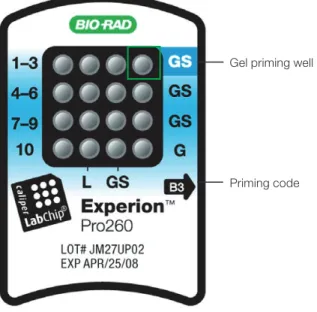
1. Pipet 12 µl GS into the top right well of the chip (highlighted and labeled GS, gel priming well) (Figure 3.1). Insert the pipet tip vertically and to the bottom of the well when dispensing. Dispense slowly to the first stop on the pipet, and do not expel air at the end of the pipetting step.

2. On the priming station, set the pressure setting to B and the time setting to 3, as specified by the alphanumeric code on the chip (Figure 3.1).

3. Open the Experion priming station and place the chip on the chip platform, matching the arrow on the chip with the alignment arrow on the chip platform. A post on the chip prevents insertion in the wrong position. Do not force the chip into position.

4. Close the priming station by pressing down on the lid. The lid should snap closed.

5. Press Start. A “Priming” message appears on the screen of the priming station, and the timer counts down. Priming requires approximately 60 sec. Do not open the priming station during countdown. 6. An audible signal and “Ready” message indicate that priming is complete. Open the priming station

and remove the chip. If the lid sticks, press down on it while pressing down on the release lever. 7. Turn the chip over and inspect the microchannels for bubbles or evidence of incomplete priming. If

the chip is primed properly, the microchannels will be difficult to see (it may be helpful to compare a primed chip to a new, unused chip). If you detect a problem, such as a bubble or incomplete priming, prime a new chip.

8. Place the chip on a clean surface for loading.

Start the run within 5 min of priming and loading the chip. For help with chip loading, refer to the Experion Training Video: Chip Loading, available in the Experion software Help section under

Contents and Index > Contents > Appendices > Technical Videos.

Bubbles forced into microchannels during priming take the shape of the microchannel and are elongated, not round.

Fig . 3 .1 . Experion Pro260 chip . The locations of the gel priming well (GS, highlighted) and alphanumeric priming code are indicated.

Gel priming well

(17)

3.7 Load the Chip

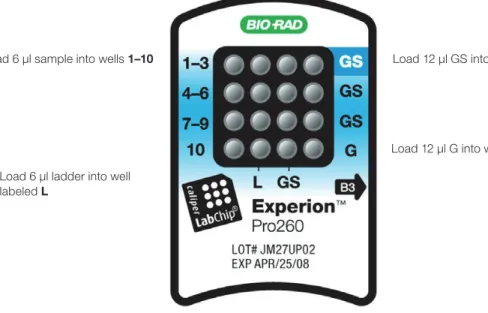
1. Using a pipet, remove and discard any remaining GS from the gel priming well. Pipet 12 µl GS into all 4 wells labeled GS (including the gel priming well, Figure 3.2).

2. Pipet 12 µl filtered gel (G) into the well labeled G (Figure 3.2). 3. Pipet 6 µl of each diluted sample into sample wells 1–10.

4. Pipet 6 µl diluted Pro260 ladder into the ladder well labeled L (Figure 3.2). Use the Pro260 ladder within 8 hr of preparation. Every chip must have Pro260 ladder loaded into the ladder well labeled L.

Fig . 3 .2 . Experion Pro260 chip . Wells for loading GS, G, samples, and ladder are indicated.

5. Inspect all wells for bubbles by holding the chip above a light-colored background and looking through the wells (Figure 3.3). Dislodge any bubbles at the bottom of a well with a clean pipet tip or by removing and reloading the solution.

6. Place the loaded chip into the Experion electrophoresis station and start the run within 5 min.

Fig . 3 .3 . Bubble formation during loading of Experion Pro260 chips . Surface bubbles do not generally cause problems during a run, but bubbles at the bottoms of wells must be removed. Left, bubbles trapped at the bottom of wells. The GS and G wells and sample wells 1, 3, and 4–6 contain no solution. Wells 8, 10, and L are filled properly and have no bubbles, but large bubbles have formed at the bottoms of wells 7 and 9 (note the difference in the diameter of the light-colored circles in wells 8 and 9). Right, bubbles have formed at the surface of the three GS wells on the right side of the chip; the rest of the wells have no bubbles.

Experion Pro260 Analysis Kit

Load 12 µl G into well labeled G Load 12 µl GS into all 4 wells labeled GS

Load 6 µl ladder into well labeled L

(18)

3.8 Run the Pro260 Analysis

1. Open the lid of the electrophoresis station by pulling the release latch. Place the primed and loaded chip on the chip platform and close the lid.

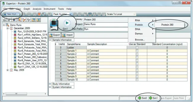
2. In the Experion software toolbar, click New Run . In the New Run screen (Figure 3.4), from the Assay pull-down list, select Protein > Protein 260.

3. Either select a project folder for the run from the Project pull-down list or create a new project folder by entering a name in the Project field or by selecting File > Project > New. The project folder appears in the project tree.

4. Enter a name for the run in the Run Prefix field and click Start Run .

5. In the New Run dialog (Figure 3.5), select the number of samples to be analyzed. Though all wells are filled, the Experion system stops the analysis when it reaches the number of samples entered.

Fig . 3 .5 . New Run dialog . The Experion system stops analysis when it reaches the number of samples entered.

Fig . 3 .4 . Details of the New Run screen . The green dot in the lower right corner indicates that communication between the electrophoresis station and Experion software has been established.

(19)

Do not open the lid of the Experion electrophoresis station until the run is complete. The lid does not lock. Opening the lid aborts the run.

An “IV Check Error” message indicates the system cannot make electrical contact in one of the wells. This often means there is a bubble at the bottom of the well. Abort the run, and check the chip for bubbles or empty wells. Refill the affected well(s), and start the run again.

7. During separation, the sample name is highlighted in the project tree and the electropherogram trace, and virtual gel bands appear in real time:

n The electropherogram of the sample being separated appears in the electropherogram

view

n The lane corresponding to that sample is outlined in pink and has a dark background

To display the electropherogram of another sample, click on either the sample name in the project tree or on a lane in the virtual gel.

8. When analysis is complete (after ~30 min), the instrument beeps and a window opens indicating the end of the run. Select OK and remove the chip from the chip platform.

9. Clean the electrodes using deionized water within 30 min of each Pro260 chip run.

3.9 Clean the Electrodes

1. Fill a cleaning chip with 800 µl deionized water (0.2 µm-filtered). Gently tap the side of the cleaning chip to remove any trapped bubbles from the wells.

2. Place the cleaning chip on the chip platform in the electrophoresis station, close the lid, and leave it closed for 1 min.

Never store the cleaning chip inside the electrophoresis station. Store the empty cleaning chip covered to keep the wells clean. A cleaning chip is included with each box of chips.

3. Open the lid, remove the cleaning chip, and allow the electrodes to dry for 1 min. Close the lid. 4. Replace the water in the cleaning chip after use to avoid contamination. For storage, remove the

water from the cleaning chip and store the chip in a clean location.

6. Click Start. The green LED in the center of the front panel on the electrophoresis station blinks, and the system performs a number of checks: it confirms that a chip has been inserted, that all wells contain liquid, that electrical connections are made, etc. A calibration counter marks the progress of these calibrations at the upper right of the screen.

(20)

3. Examine the separation of at least one sample. Click on the sample name in the project tree or on the lane in the virtual gel to view the electropherogram, which should have the following features:

n Two well-resolved marker peaks and a set of system peaks

n Sample peaks located between the system peaks and upper marker n Flat baseline

If the upper and lower marker peaks are not properly assigned, you may need to include or exclude peaks, or manually set the marker (see Section 6.3).

4. Evaluate the data analysis performed by Experion software (see Chapter 4, Data Analysis). If necessary, change the analysis settings and parameters — including protein quantitation methods — by following the instructions in Chapters 5 and 6.

3.10 Evaluate the Run

When a run is complete, evaluate the run and the analysis of the data by Experion software. 1. Ensure all lanes (ladder and samples) are visible in the virtual gel. The markers (indicated by pink

triangles) should be visible in and aligned across all lanes. If the marker peaks are not properly assigned, you may need to include or exclude peaks, or manually set the marker (see Section 6.3). 2. Evaluate the separation of the Pro260 ladder. To display the ladder electropherogram, click the

ladder well in the project tree, or click on the lane labeled L in the virtual gel. The electropherogram should resemble the one shown in Figure 3.6 and should have the following features (if your ladder does not have these features, see Chapter 7, Troubleshooting for more information):

n Two marker peaks and a set of system peaks

n Eight Pro260 ladder peaks between the system peaks and upper marker n Flat baseline

n Marker peaks at least 20 fluorescence units above the baseline

Fig . 3 .6 . Separation of the Pro260 ladder . Note the flat baseline and well-resolved peaks. All identified peaks are numbered, and the lower and upper markers are indicated by green asterisks (*). The 260 kD protein in the Pro260 ladder is labeled as the upper marker in the Results table.

Pro260 ladder peaks

Baseline Upper marker Lower marker

(21)

Data Analysis

4

This chapter outlines the basic steps and software features used to view and analyze data. For a more detailed description of Experion™_{software and its various functions, refer to the software Help}

menu. For information on how to customize analysis parameters, refer to Chapter 6, Changing Analysis Settings and Parameters.

(22)

4.1 Viewing Data

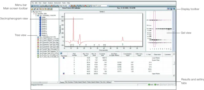
The main window of the Experion software user interface contains menus and toolbars, a tree view, and three data views: the electropherogram view, gel view, and results and settings tabs. (Figure 4.1).

4.1.1 Managing Run Files and Project Folders in the Tree View

The tree view (Figure 4.2) displays the project tree, a hierarchical tree of all projects and the data files they contain. Use the project tree and the toolbar above it to:

n Open run files and select samples for viewing n Create project folders

n Export and import one or more run files n Edit names of run files and project folders n Move runs into project folders

n Delete run files and project folders

Fig . 4 .1 . Main window of Experion software . The toolbars, menus, and data views are indicated.

Menu bar

Main screen toolbar Display toolbar Electropherogram view

Tree view Gel view

Results and settings tabs

Fig . 4 .2 . Tree view details . The project folder name, sample well label, and run file prefix can be customized.

Toolbar

Run file Sample Project folder

(23)

To open a run file, double-click on it. The run file opens, displaying the electropherogram and Results tab for the Pro260 ladder, and the virtual gel for the entire run.

To view the data from a sample, click on the sample name or select the corresponding lane in the gel view.

To edit a run file or project folder name, right-click on it and select Rename Project or Rename Run. Type in the new name.

To import, export, move, or delete files and folders, click the ocons in the toolbar or use the context menu accessed by right-clicking on the items in the tree view. For more details, refer to the Experion software Help file.

4.1.2 General Display Controls

Data in the electropherogram view, gel view, and results and settings tabs are linked. Selecting a sample or peak in one area automatically opens or highlights that sample/peak in the other two areas. To adjust the relative sizes of the three data views and the tree view, click on and drag the border of the view to its new location.

To hide or show one of the three data views, click on the corresponding icon in the display toolbar (located in the upper-right corner of the display, just above the gel view (Figure 4.1).

To zoom in on (expand the view of) a portion of an electropherogram or virtual gel, click on the corner of the area that you would like to enlarge and mouse over to the opposite corner. Double-click anywhere in the electropherogram view to return to the previous view.

4.1.3 Electropherogram View

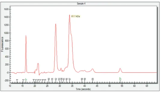
Experion software plots fluorescence intensity versus migration time to generate an electropherogram for each sample. In the electropherogram, peaks identified by Experion software are numbered (Figure 4.3). Peaks generated by the markers and used for normalization (for example, the lower and upper markers) are numbered in green and labeled with an asterisk.

To view the calculated size of a peak or other area of an electropherogram, place the cursor over the peak/area (Figure 4.3). To display the sizes of all the peaks in the electropherogram, select Molecular Weight in the Select Peak Information pull-down list (main screen toolbar).

Fig . 4 .3 . Example of an electropherogram . All identified peaks are numbered, and the lower and upper markers are indicated by a green asterisk (*). Place the cursor over a peak to reveal its size.

(24)

Single-Well View

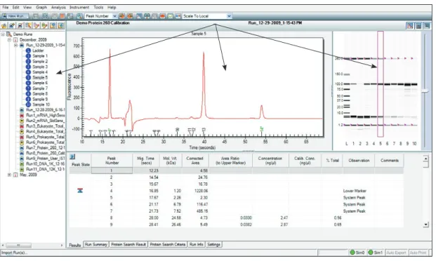
This is the default view, which shows the electropherogram data from a single well (Figure 4.4). To return to this display:

1. Click on the sample in the project tree or on the corresponding lane in the virtual gel. 2. In the main screen toolbar, click View Single Well or select View > Single Well. 3. The electropherogram appears. The corresponding lane in the virtual gel is outlined in pink.

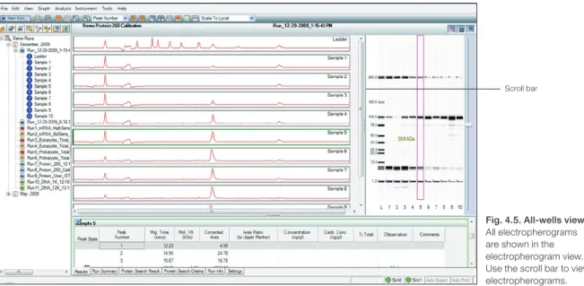
All-Wells View

To display all electropherograms simultaneously (Figure 4.5):

1. In the main screen toolbar, click View All Wells or select View > All Wells.

2. Electropherograms for each sample populate the electropherogram view (Figure 4.5). Use the scroll bar to scroll through the electropherograms, or minimize the results and settings table to accommodate the multiple electropherograms.

3. To select and expand a particular electropherogram, double-click on it. The data appear in a single-well view.

Fig . 4 .4 . Single-well view . As indicated by the arrows, a single electropherogram appears, the name of the sample is highlighted in the project tree, and the corresponding lane in the virtual gel is outlined.

Double- or right-click on a peak to select it. An inverted black arrow appears above the peak in the electropherogram, and a pink arrow appears above the corresponding band in the virtual gel. The peak number and corresponding data also appear highlighted in the Results table.

Display electropherograms in three different ways:

n One at a time (single-well view)

n All at once in separate windows (all-wells view) n As superimposed images (overlays)

(25)

Fig . 4 .5 . All-wells view .

All electropherograms are shown in the electropherogram view. Use the scroll bar to view electropherograms.

Electropherogram Overlays

Superimpose (overlay) multiple electropherograms to facilitate direct comparison among profiles. To overlay a subset of electropherograms (Figure 4.6), use one of the following options:

n Move into the single-well view and, in the main screen toolbar, click Start Overlay .

Select wells (lanes) in the virtual gel. Each gel lane that is displayed in the electropherogram is outlined. To end the overlay, click End Overlay

n Select the lanes in the virtual gel while holding the Ctrl key (for noncontiguous, individual

lanes) or the Shift key (for lanes next to the original lane selected). To exit, click on a lane in the virtual gel or on a sample name in the project tree

n Select Analysis > Start Overlay. Select the lanes to overlay. To end the overlay, select

Analysis > End Overlay

Electropherograms appear superimposed in a single window, each in a different color. (The colors cannot be changed.) The sample name appears at the top of the electropherogram, in a color that corresponds to the trace. The fluorescence scale of the overlay electropherogram is based on the sample that is selected first; therefore, select the sample with the highest peaks first.

Fig . 4 .6 . Electropherogram overlay . Electropherograms are shown in different colors, and the corresponding lanes in the virtual gel are outlined. In this example, lanes 2, 5, and 7 are superimposed using the overlay feature.

(26)

Peak Labels

Experion software automatically labels detected peaks with numbers for easy identification, and the upper and lower markers used for normalization are indicated in green and with an asterisk (*). To change the type of label displayed, select Graph > Peak Info (or use the pull-down list in the main screen toolbar) and select one of the following options:

n No Peak Info — displays no peak information

n Peak Number — uses sequential numbers for peak identification (default selection) n Peak Time — uses peak migration time (min:sec) for peak labels

n Peak Height — uses peak height in units of fluorescence intensity for peak labels n Peak Cor . Area — uses calculated (corrected) peak area for peak labels

n Molecular Weight — uses calculated mass (molecular weight, kD) for peak labels n Peak Concentration — uses calculated relative concentration (ng/μl) for peak labels

Electropherogram Tags (Annotations)

To annotate a peak in the electropherogram, right-click on the peak and select Add Tag (Figure 4.7). A tag is automatically generated with the peak information selected (for example, peak number). To edit a tag, right-click on it, select Edit Tag, and change the information. Click OK .

To annotate a region in the electropherogram, right-click in the region and select Add Tag. In the

Edit Tag dialog, enter the annotation and click OK .

To move a tag, click and drag the label to the desired place in the electropherogram.

Fig . 4 .7 . Example of tagged (annotated) peaks in an electropherogram .

(27)

Technical Support: 1-800-4BIORAD • 1-800-424-6723 • www.bio-rad.com 23 4.1.4 Gel View

Experion software converts electropherogram data into densitometric bands, which appear in the virtual gel (Figure 4.8). Each lane of the virtual gel corresponds to a different sample, and all samples from a chip are shown in a single gel view. When a sample is selected for view as an electropherogram, the corresponding lane in the virtual gel is outlined in pink.

Place the cursor over an area in the virtual gel to view its estimated size in kilodaltons (“kDa”). If a band corresponds to a peak identified by Experion software, view the peak number and calculated size, concentration, and percentage of total protein by placing the cursor over the band (Figure 4.8).

Right-click on a band to select it. A pink arrow appears above the selected band in the virtual gel, and an inverted black arrow appears above the corresponding peak in the electropherogram. The peak number and corresponding data also appear highlighted in the Results table. Only one peak can be selected at a time.

To select a different color scheme, choose View > Gel Color and select a color from the list. By default, the gel view displays bands as black signals on a white background.

To change the contrast of the bands, use the sliding cursor (Figure 4.8). Changing the contrast does not change the data, but it may improve visualization of faint bands in the virtual gel.

Fig . 4 .9 . Results and settings . Shown is the Results table for a single sample.

4.1.5 Results and Settings

The six results and settings tabs (Figure 4.9) present options for viewing, customizing, and analyzing the separation data (see Section 4.3, Using Results and Settings to View and Annotate Data).

Fig . 4 .8 . Gel view . Place the cursor over a band in the gel view to display the peak number, size, concentration, and % of total protein. Move the sliding cursor to adjust band intensity.

(28)

4.2 Changing the Fluorescence Intensity Scale

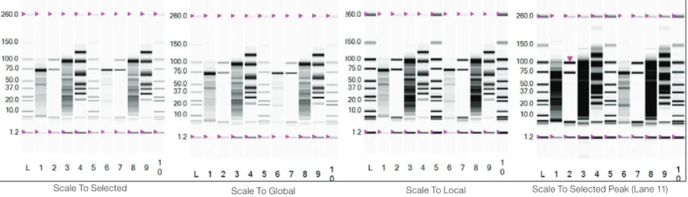
To display more or less detail in the electropherogram traces and lanes in the virtual gel, use the options available under the Graph menu, which determine the scale used for the y-axis (fluorescence intensity) of electropherograms and define the relative scale intensity of the lanes in the virtual gel (Figure 4.10):

n Scale To Selected — uses the fluorescence value of the tallest peak in a selected

electropherogram to set the scale of the y-axis for all the other samples. Use this option when comparing (overlaying) a sample with a high-intensity peak and one with a less intense peak

n Scale To Global — uses the fluorescence value of the tallest peak from all samples to set

the scale of the y-axis for all the samples. Use this option to adjust the virtual gel to be most similar to an SDS-PAGE separation

n Scale To Local (default) — uses the fluorescence value of the tallest peak in each

electropherogram to set the scale of the y-axis for that electropherogram: each sample is scaled separately. This is the best way to view protein electropherograms and sample details

n Scale To Selected Peak — uses the fluorescence value of the selected peak to set the

scale of the y-axis for all samples

Fig . 4 .10 . Options for modifying the fluorescence intensity scale . Examples of how each option affects the display of a virtual gel are shown.

Scale To Global Scale To Local Scale To Selected Peak (Lane 11) Scale To Selected

(29)

4.3 Using Results and Settings to View and Annotate Data

The following options appear under the results and settings tabs:

n Results — summarizes analysis data for all detected peaks. The data in this table can be

exported (see Section 4.5.2, Exporting Data Files to Other Applications). To view the results of a particular sample, click the electropherogram in the all-wells view or lane in the gel view, or select that sample from the project tree. Alternatively, use the arrows in the main screen toolbar to navigate through the samples. See below for instructions on how to customize the types of data shown under this tab

n Run Summary — displays a run summary for all wells; right-click to export the data n Protein Search Result — summarizes user-defined known proteins: lists the samples

that contain a peak that fits with the search of size, or molecular mass as defined under the Protein Search Criteria tab and performs statistical calculations for the size, concentration, and percentage of total protein for each peak identified

n Protein Search Criteria — used to compare statistics for specific proteins in the samples

(see Section 6.1, Designating and Searching for Specific Proteins for information on how to designate and then search for known proteins)

n Run Info — used to enter sample names and comments after a run is finished (see below

for instructions)

n Settings — used mostly for troubleshooting, but can be used to edit the parameters used

to identify peaks (see Section 6.5, Changing Peak Finding Parameters, or the Experion software Help file for more details about these settings)

To customize the types of data shown under the Results tab:

1. Right-click on any of the column headers in the Results tab (or click the arrow to the left of the column header). The Column Selector dialog opens.

2. Use the arrow keys to show, hide, or change the order of display of any of the available headers. For detailed explanations of each setting, refer to the software Help file.

3. Click OK to save the changes, or click Cancel to close the dialog without saving the changes. Under the Results tab, total concentration data appear at the bottom of the table. This calculation represents the total protein concentration of the original sample. See Bio-Rad bulletins 5299, 5784, and 5423 to learn more about comparing these calculations to data gathered by other methods. To enter sample names and descriptions:

1. Click the Run Info tab and then click on the plus sign (+) next to Sample Information. 2. Click on any active cell, enter the sample names and descriptions, and click Apply. Click

File/Save to save the changes. The sample name appears above its electropherogram. To enter other information about the experiment:

1. In the Run Info tab, click the plus sign (+) next to the Study Information and/or System Information area(s).

2. Double-click in any blank field, enter the information, and click Apply. Click File/Save.

(30)

4.4 Comparing Data from Different Runs

Experion software allows you to overlay runs from different chips (same assay type), enabling direct comparison of electropherograms and virtual gels from multiple chips. You can save and edit this new virtual chip, but you will not be able to make any new calculations. All calculations in the Results table carry over from the original runs.

Experion software accepts up to 40 samples for comparison (the default is 30). To change the number of wells used, select Tools > Options. Under the Advanced tab, change the number under Visible Compare Runs Gel lanes.

Only one ladder can be used per comparison. If a ladder is not selected, the ladder used in the first run file is used as the ladder for the entire virtual chip. If an additional ladder is inserted in the virtual chip, it is treated as a sample.

1. Click Create a New Compare Run or select Analysis > New Compare Run. In the Compare Runs Setting dialog, enter a name for the comparison in the Compare Name field.

2. Select the project in which you wish to store the comparison from the Target Project pull-down list. 3. Select the assay from the Assay Type pull-down list and click Next. The Compare Runs dialog

opens, displaying only runs of the same assay type.

4. Double-click to expand the run files you want to compare, or select a run file and click List Samples. 5. Click the run file or sample(s) and use the arrows to move them to and from the Compare field.

To select several lanes at a time, click the sample names while holding the Ctrl or Shift key. To open a window displaying the selected samples in a gel view, click Show Gel Lanes.

In security mode, all run comparisons are saved and cannot be deleted.

6. Select Realign Data to align the results of all the runs and click OK. The separations appear together in one window as a single experiment. In the Results table, the sizes and concentrations for proteins in each sample are unchanged; the original sizes and concentrations are shown.

7. To change the lanes used in the run comparison:

a. Open a run comparison by double-clicking the file name in the tree view and then clicking Edit Compare Run or selecting Analysis > Edit Compare Run .

b. Select the samples you want to add or delete, and use the arrows to add or remove them from the comparison.

c. To view the samples within a run, double-click the run file or select it and click List Samples. 8. Click OK to process the changes and view the results.

(31)

4.5 Saving, Exporting, and Printing Data

4.5.1 Saving Data Files

Data are automatically saved to a run file. Names for run files are given according to the selection made in the Run Files tab of the Options dialog.

To designate a new name for a file, select File > Save As and enter the desired name.

To view the selections or make changes in the automatic naming of files, select Tools > Options > Run Files. The following options appear:

n Create Run name by combining — select the options to be added to the file name.

Options include the prefix (enter the desired characters), assay class (adds the assay type to the file name), instrument name, date, and time

n Run file folder — choose between default (saves files to the directory C:\Program Files\

BioRad Laboratories\Experion Software\Data) and custom (enables navigation and selection of another folder)

n Create daily folders — select to enable creation of daily subfolders by date. When this

option is selected, the software stores all run files from the same date in a single folder

4.5.2 Exporting Data Files to Other Applications

To export data to another program (for example, Excel software), select File > Export Data. In the

Export dialog, select the desired options. For a complete description of all export options, refer to the Experion software Help file.

To export files automatically after a run is completed: 1. Select Tools > Options and click the Advanced tab. 2. Select Auto Export and then click Settings .

3. Select the options for Auto Export and click Apply.

To quickly copy and paste electropherograms, virtual gels or lanes in the gels, or data tables into another application, use the options under the Edit pull-down list.

4.5.3 Printing Data Files

You can print both graphic and tabulated data from a run.

To choose the print options, select File > Print and select the desired options in the Print dialog. For a complete description of all printing options, refer to the Experion software Help file (search term “printing data”).

To print files automatically after a run is completed: 1. Select Tools > Options and click the Advanced tab. 2. Select Auto Print and then click Settings.

3. Choose the desired options in the Experion Print dialog and click Apply. To save or print the data as a PDF file, select File > Print and select Print PDF.

(32)

(33)

Protein Quantitation

Methods

5

(34)

5.1 Protein Quantitation Methods

Experion™_{software enables protein quantitation by several approaches. The selection of approaches}

depends on the type of experiment and desired level of accuracy (Table 5.1). Refer to Appendix A and bulletin 5784 for details about the different quantitation methods.

Table 5.1. Protein quantitation methods used by Experion software. Absolute quantitation methods provide greater accuracy than relative quantitation methods. The accuracy of percentage determination is protein dependent.

Calibration Method and Internal Standard Used Single-Point Calibration Curve Quantitation Method Output Upper Marker User-Defined Upper Marker User-Defined Percentage Determination % Total No internal standard required

Concentration Determination

Relative quantitation ng/µl l — — —

— l — —

Absolute quantitation ng/µl — — l —

— — — l

5.2 Performing Percentage Determination

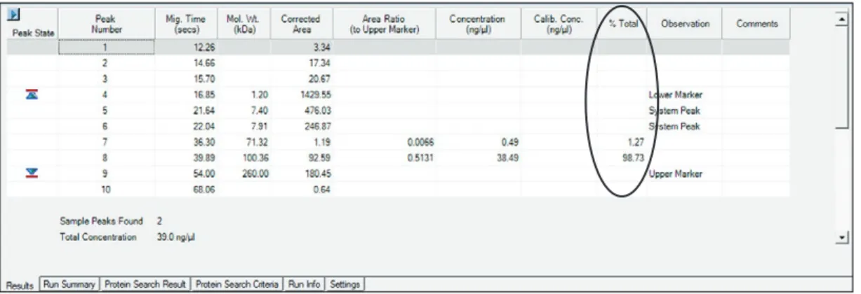
Experion software automatically calculates a percentage of total protein (% total) value for each detected peak and lists the results in the % Total column of the Results table (Figure 5.1). Click on the peak of interest in the electropherogram to highlight the data for that peak.

Fig . 5 .1 . Results table showing quantitation data for peaks in a sample . Experion software automatically performs % total and relative concentration determinations for each peak identified in every sample.

To exclude a peak from the % total calculation, right-click on the peak (in either the single-well electropherogram view or Results table) and select Exclude Peak in the context menu. The new calculations for the remaining peaks appear in the Results table.

This change affects a selected sample. To exclude multiple peaks from multiple samples, use the

Settings tab and the Peak Find Settings options in the All Wells Settings dialog (see Section 6.4, Excluding a Peak From Analysis and 6.5, Changing Peak Finding Parameters) and adjust the peak detection criteria.

(35)

5.3 Performing Relative Quantitation

Experion software also automatically performs quantitation of all peaks in a sample by a single-point calibration to the 260 kD upper marker and presents these data in the Concentration (ng/µl) column of the Results table.

To view these default relative quantitation results, click on the peak of interest in the electropherogram to highlight the data for that peak.

To perform relative quantitation against a different, user-defined internal standard:

n Add the standard to the samples at a single concentration, and n Change some of the analysis settings in the software

Selection of the user-defined standard in the software may be done after the run is complete. This enables easy comparison of the relative quantitation results derived by using both the upper marker and the user-defined standard.

To perform relative quantitation with a single concentration of a user-defined internal standard: 1. Prepare the protein samples and reagents as outlined in Section 3.5, except add a known

concentration of the internal standard (for example, 500 ng/µl) to each sample. For example, replace half the volume of sample with the internal standard (combine 2 µl sample, 2 µl internal standard, and 2 µl sample buffer).

Fig . 5 .2 . Internal Std . and Std . Protein Calibration Curve window.

Do not add the internal standard to the Pro260 ladder. 2. Run the Pro260 analysis.

3. After evaluating the run as described in Section 3.10, select Analysis > Internal Std . and Std Protein Calibration Curve.

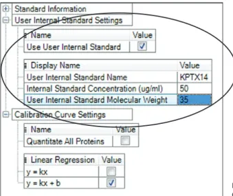
4. In the Internal Std . and Std . Protein Calibration Curve window (Figure 5.2), select Use User Internal Standard and enter the name, concentration, and molecular weight (MW) of the internal standard. Click Apply and then Close. The new concentrations appear in the Results table under the Concentration (ng/µl) column (Figure 5.3).

(36)

5.4 Performing Absolute Quantitation

Experion software also allows quantitation using a calibration curve generated by a range of known concentrations of that protein (absolute quantitation). In this method:

n Different concentrations of the protein are separated in different sample wells

n The peak areas of the different concentrations are compared to the peak area of an internal

standard. As with relative quantitation, either the upper marker or a user-defined protein can be used as the internal standard

n The protein concentrations in the samples are then determined from this calibration curve

Experion software displays the results for both relative and absolute quantitation, enabling easy comparison of the accuracy achieved by these different approaches.

5.4.1 Absolute Quantitation Using the Upper Marker as Standard

1. Prepare a dilution series of 3–6 different concentrations of the protein used for calibration. The total protein concentration in each sample must be within the linear dynamic range of the assay. Prepare these samples with the other samples for Pro260 analysis as described in Section 3.5.

2. In the Run Info tab under Sample Information, designate the wells that contain the proteins for the calibration curve by selecting them in the Use as Standard column (Figure 5.4). Enter their concentrations in the Standard Concentration column and click Apply.

3. Run the Pro260 analysis.

Fig . 5 .3 . Results from relative quantitation.

(37)

4. After evaluating the run as described in Section 3.10, select Analysis > Internal Std . and Std Protein Calibration Curve.

5. In the Internal Std . and Std . Protein Calibration Curve window (Figure 5.5), do the following: a. Under Standard Information, next to Standard Protein Molecular Weight, enter the MW corresponding to the region where the software searches for a peak, for both the calibrants and the samples. The software checks for a peak in the sample wells that has the entered value (± 5%). If necessary, modify the concentrations of the calibrants by double-clicking on the concentration value and typing in a new value.

b. Ensure that Use User Internal Standard is not selected.

c. Under Calibration Curve Settings, if the protein used for calibration (calibrant) is different or has a different mass than the protein being quantitated, select Quantitate All Proteins and click

Apply. If you do not do this, the software only reports absolute concentrations for peaks that are the same size as the calibrant.

d. Under Calibration Curve Settings, select the Linear Regression to be used.

e. Click Apply to update the calculation. The calibration curve appears and displays the equation for the linear regression (Figure 5.5). The table below the graphic displays data for the wells containing the standards. Click Close.

6. In the Results tab, the concentration for each protein identified by Experion software is derived by relative quantitation against the 260 kD upper marker and automatically appears in the

Concentration column; the calibrated concentrations of proteins found in the specified region appear in the Calib . Conc . column.

Fig . 5 .5 . Internal Std . and Std Protein Calibration Curve window . In this example, a 100 kD protein is used to build a 5-point calibration curve for quantitating a 100 kD sample protein.

(38)

5.4.2 Absolute Quantitation Using a User-Defined Internal Standard

This is the most stringent method of quantitation. It combines two of the approaches described above:

n A calibration curve is generated using known concentrations of a protein, and n A user-defined protein is used as the internal standard

1. Prepare a dilution series of 3–6 concentrations of the protein that you will use for calibration. 2. Add a known concentration of the internal standard to each sample (except the Pro260 ladder),

including those that will be used for calibration. Prepare these samples and other samples as described in Section 3.5.

3. Under the Run Info tab, designate the wells that contain the proteins for the calibration curve and enter their concentrations (Figure 5.5). Click Apply and run the Pro260 analysis.

4. After evaluating the run as described in Section 3.10, select Analysis > Internal Std . and Std Protein Calibration Curve .

5. In the Internal Std . and Std . Protein Calibration Curve window (Figure 5.5), do the following: a. Under Standard Information, next to Standard Protein Molecular Weight, enter the MW corresponding to the region where the software searches for a peak, for both the calibrants (standards) and the samples. The software checks for a peak in the sample wells that has the entered value (± 5%). If necessary, modify the standard concentrations by double-clicking on the concentration and entering a new value.

b. Select Use User Internal Standard and enter the name, concentration, and size of the internal standard. Click Apply.

c. Under Calibration Curve Settings, if the protein used for calibration (calibrant) is different or has a different mass than the protein being quantitated, select Quantitate All Proteins and click

Apply. If you do not do this, the software only reports absolute concentrations for peaks that are the same size as the calibrant.

d. Under Calibration Curve Settings, select the Linear Regression to be used. Click Apply to update the calculation.

6. The calibration curve appears, displaying the equation for the linear regression. The table below the graphic displays the data for the protein standard samples. Click Close.

7. In the Results table, the concentration for each protein derived by relative quantitation against the user-defined internal standard appears in the Concentration column, and the calibrated concentration (using the calibration curve in conjunction with the user-defined standard) appears in the Calib . Conc . column.

(39)

Changing Analysis

Settings and Parameters

6

Once an Experion™_{analysis is complete and you have examined the quality of the run and of the}

data, you can reanalyze the data by changing some of the settings. Most of the steps outlined in this chapter are used for troubleshooting purposes or are optional; they are not required in most analyses.

(40)

6.1 Designating and Searching for Specific Proteins

1. Designate and search for specific proteins in your samples:

a. In the Protein Search Criteria tab, click Add Protein Name , or in the electropherogram, right-click on a peak and select Add to Protein Search Criteria. The Protein Search Criteria

tab opens and contains the mass and tolerance range for that entry. b. Click in the field under Protein Name and enter the protein name. c. Click in the field under Mol Wt and enter the size of the protein in kD.

d. Click in the field under the ±s mass column to enter the new value for the tolerance in kD and exclude wells that are not relevant to the search.

2. A list of all the peaks that fit the criteria appears in the Protein Search Result tab. Separate tables appear for each protein designated in the search criteria list. To exclude a peak, right-click on the peak name in the table and select Exclude Peak.

3. To delete designated proteins (“protein names”) from a search, click Delete Protein Name in the toolbar of the Protein Search Criteria tab.

6.2 Changing Protein Quantitation Parameters

Experion software uses relative quantitation against the upper marker to calculate the concentrations of all the peaks detected in a sample. The calculated concentrations appear in the Results table, under the

Concentration (ng/µl) column.

For more information about protein quantitation, including about how to perform relative quantitation against a user-defined standard or to perform absolute quantitation using a calibration curve, refer to Appendix A and the instructions provided in Chapter 5, Protein Quantitation Methods.

6.3 Manually Setting a Marker

To designate a peak as a marker (and change the alignment of a sample), right-click on the peak in either the electropherogram (single-well view) or the Results table and select Manually Set Lower Marker or Manually Set Upper Marker to define the peak as the new lower or upper marker. Do this if no or incorrect peaks have been selected as the lower or upper marker.

Pink triangles in the virtual gel indicate markers. The markers should be aligned across all lanes.

6.4 Excluding a Peak from Analysis

To exclude one or more peaks from analysis of a single sample, right-click on the peak in either the electropherogram (single-well view) or Results table and select Exclude Peak from the context menu. This change affects only a selected sample.

To exclude multiple peaks from multiple samples, open the Settings tab and use the Peak Find Settings options in the All Wells Settings dialog (see Section 6.5, Changing Peak Finding Parameters) to adjust the criteria by which peaks are detected.

Excluded peaks are not included in total protein calculations. Therefore, excluding a peak from analysis affects percentage determination (% total calculations) for the other peaks in a sample.

(41)

6.5 Changing Peak Finding Parameters

The parameters entered tell the peak-find algorithm whether a peak is significant.

To edit the parameters used by Experion software for finding peaks in a selected sample/well:

1. Select the sample by clicking on the lane in the virtual gel (or on the sample name in the tree view). 2. Under the Settings tab, edit the parameters under Peak Find Settings:

n Slope Threshold — represents the variation in fluorescence units over time required to

detect a peak (accepted values are 0.2–1,000, with lower values yielding more peaks)

n Min . Peak Height — minimum height required for a peak to be integrated (accepted values

are 0.1–1,000). Determine the appropriate value for this parameter by zooming in on a small peak in an electropherogram and reading its fluorescence value on the y-axis

n Min . Peak Width — minimum amount of time that must elapse before a peak is

recognized (accepted values are 0.1–10, with lower values yielding more peaks)

3. Click Apply to apply the changes and reanalyze the data. Click Save in the main screen toolbar to save the new conditions or click Reset to Default to recover the default settings.

To modify the peak-find settings for all sample wells:

1. Under the Settings tab, click the All Well Settings tab or select Analysis > All Wells Settings. 2. In the All Wells Settings dialog, expand Peak Find Settings and select the type of modification you

would like to apply (see above for descriptions).

3. Click OK to apply changes and Yes to overwrite the settings. Click Save in the main screen toolbar to save the new conditions. To reset to default settings, click Reset to Default.

Do not adjust the Peak Find Settings values so that the markers are eliminated from analysis.

6.6 Changing General Settings

These settings appear in the Settings tab, in the All Wells Settings dialog under General Settings

(Figure 6.1). They apply to all samples in a run.

n Data Frequency — displays the rate of data collection in Hz

n Display Start Time — displays the time Experion software begins displaying peaks n Display End Time — displays the time Experion software stops displaying peaks n Upper Marker Concentration — displays the concentration of the upper marker

n Use Time Corrected Areas — corrects for peaks of different sizes that pass the detector

at different rates

n Calibrate All Valid Peaks — select this option if you are running a calibration curve and

want Experion software to calibrate all peaks (this is the same as selecting Quantitate All Proteins in the Internal Std . Protein Calibration Curve window)

n Filter Width — determines the width of the polynomial (in sec) to be applied to the data for

filtering (noise reduction). Set this variable to less than twice the width of peaks. Valid values are 0.3–10

n Polynomial Order — defines the power series applied to fit the raw data. Valid values are

1–10, with lower values yielding smoother curves

(42)

6.7 Baseline Modification

To change the method used by Experion software for adjusting the baseline in a selected electropherogram (single sample):

1. Under the Settings tab, select one of the following two options under Algorithm Inclusion Settings

(Figure 6.2):

n Baseline Correction — (default) subtracts the baseline from the signal. The baseline

represents a slow, rolling component in the signal. Generally, this method affects the original shape of the curve and subsequent calculations. The more complex the baseline, the greater impact subtraction might have on the signal. However, for well-resolved peaks with a slow rolling component, this method can normalize calculations across the chip. If peaks are poorly resolved, baseline correction can cause considerable artifacts

n Zero Baseline — subtracts the average baseline value from the signal. This method

does not affect the shape of the curve; it shifts the baseline down to zero. If the Baseline Correction option results in undesirable artifacts (small peaks do not appear, or too many peaks appear), change this setting to see if it remedies the problem

Fig . 6 .1 . General Settings options .

2. Click Apply to apply the changes and reanalyze the data, and click Save in the main screen toolbar to save the new conditions or choose Reset to Default to recover the default settings.

To edit the parameters used by Experion software for adjusting the baseline for all samples: 1. Either open the Settings tab or select Analysis > All Wells Settings.

2. In the All Well Settings dialog, expand Algorithm Inclusion Settings and select the type of modification you would like to apply (see above for descriptions or Figure 6.2). Click OK.

3. In the Experion Application dialog, click OK and Yes to to overwrite the sample settings. Click

Save in the main screen toolbar to save the new conditions. To reset to default settings, click

Reset to Default in the Settings tab under All Well Settings.

Deselecting both options makes the original signal(s) appear. Sometimes it is important to see the difference between the signals across the chip if no correction is applied.

(43)

6.8 Turning Analysis Off

To turn analysis off, select Analysis > Turn Analysis Off. Analysis remains off for all runs until it is turned back on.

Turning analysis off displays the raw data from a run; it deactivates alignment, shifting the positions of the upper and lower markers in each sample. In addition, the pink arrows (in the virtual gel) indicating the positions of the markers appear only in the ladder lane. With analysis off, the migration of the

markers may not be perfectly aligned and the position of the upper marker may drift (Figure 6.3). Turning analysis off can help reveal if a problem is isolated (one or a few wells have markers out of alignment) or is general (alignment problems across the entire chip).

Fig . 6 .2 . Algorithm Inclusion Settings window .

Fig . 6 .3 . Effects of turning analysis off for two samples .

(44)

Fig . 6 .4 . Manual integration mode indicates the beginning and end of peak baselines with blue dots .

6.9 Manual Peak Integration

This function enables definition or refinement of peak areas for the ladder and all sample lanes.

1. Select a sample and click or select Analysis > Manual Integration to start manual integration. 2. Adjust the baseline by clicking and dragging the dots at the ends of the peaks (Figure 6.4).

If a peak in the electropherogram is not detected by the software, right-click on that peak and select

Add Peak. Zoom in on the peak for a better view of the baseline.

3. Save any changes by selecting File > Save Run As (use a new file name), or revert to the original baseline and integration by clicking .

Manual integration applies to individual sample wells. Moving back to automated integration loses changes made during manual integration unless those changes are saved.

(45)