Big Data Dimensional Analysis

Big Data Dimensional Analysis

Vijay Gadepally & Jeremy Kepner

{vijayg, jeremy}@ ll.mit.edu

Abstract—The ability to collect and analyze large amounts of data is a growing problem within the scientific community. The growing gap between data and users calls for innovative tools that address the challenges faced by big data volume, velocity and variety. One of the main challenges associated with big data variety is automatically understanding the underlying structures and patterns of the data. Such an understanding is required as a pre-requisite to the application of advanced analytics to the data. Further, big data sets often contain anomalies and errors that are difficult to know a priori. Current approaches to understanding data structure are drawn from the traditional database ontology design. These approaches are effective, but often require too much human involvement to be effective for the volume, velocity and variety of data encountered by big data systems. Dimensional Data Analysis (DDA) is a proposed technique that allows big data analysts to quickly understand the overall structure of a big dataset, determine anomalies. DDA exploits structures that exist in a wide class of data to quickly determine the nature of the data and its statical anomalies. DDA leverages existing schemas that are employed in big data databases today. This paper presents DDA, applies it to a number of data sets, and measures its performance. The overhead of DDA is low and can be applied to existing big data systems without greatly impacting their computing requirements.

Keywords—Big Data, Data Analytics, Dimensional Analysis I. INTRODUCTION

The challenges associated with big data are commonly referred to as the 3 V’s of Big Data - Volume, Velocity and Variety [1]. The 3 V’s provide a guide to the largest outstanding challenges associated with working with big data systems. Big datavolumestresses the storage, memory and compute capac-ity of a computing system and requires access to a computing cloud. The velocity of big data velocity stresses the rate at which data can be absorbed and meaningful answers produced. Big data varietymakes it difficult to develop algorithms and tools that can address that large variety of input data.

The MIT Supercloud infrastructure [2] is designed to address the challenge of big data volume. To address big data velocity concerns, MIT Lincoln Laboratory worked with various U.S. government agencies to develop the Common Big Data Architecture and its associated Apache Accumulo database. Finally, to address big data variety problems, MIT Lincoln Laboratory developed the D4M technology and its associated schema [3] that is widely used across Accumulo community.

While these techniques and technologies continue to evolve with the increase in each of the V’s of big data, analysts who

This work is sponsored by the Assistant Secretary of Defense for Research and Engineering under Air Force Contract #FA8721-05-C-0002. Opinions, interpretations, recommendations and conclusions are those of the authors and are not necessarily endorsed by the United States Government

978-1-4799-6233-4/14/$31.00 ©2014 IEEE

work with data to extract meaningful knowledge have realized that the ability to quantify low level parameters of big data can be an important first step in an analysis pipeline. For example, in the case of machine learning, removing extraneous dimensions or erroneous records allows the algorithms to focus on meaningful data. Thus, the first step of a machine learning analyst is manually cleaning the big dataset or performing dimensionality reduction through techniques such as random projections [4] or sketching [5]. Such tasks require a coherent understanding of the data set which can also provide insight into any weaknesses that may be present in a data set. Further, detailed analysis of each data set is required to determine any internal patterns that may exist.

The process for analyzing a big data set can often be summarized as follows:

1) Learn about data structure through Dimensional Data Analysis (DDA);

2) Determine background model of big data;

3) Use data structure and background model for fea-ture extraction, dimensionality reduction, or noise removal;

4) Perform advanced analytics; and 5) Explore results and data.

These steps can be adapted to a wide variety of data and borrow heavily from the processes and tools developed for the signal processing community. The first two steps in this process provide a high level view of a given data set - a very important step to ensure that data inconsistencies are known prior to complex analytics that may obscure the existence of noise. Traditionally, this view is obtained as a byproduct of standard database ontology techniques, whereby a database analyst or data architecture examines the data in detail prior to assembling the database schema. In big data systems, data can change quickly or whole new classes of data can appear unexpectedly and it is not feasible for this level of analysis to be employed. The D4M (d4m.mit.edu) schema addresses part of this problem by allowing a big data system to absorb and index a wide range of data with only a handful of tables that are consistent across different classes of data. An added byproduct of D4M schema is that common structures emerge that can be exploited to quickly or automatically characterize data.

Dimensional Data Analysis (DDA) is a technique to learn about data structure and can be used as a first step with a new or unknown big data set. This technique can be used to gain an understanding of corpus structure, important dimensions, and data corruptions (if present).

The article is organized as follows. Section II describes the MIT SuperCloud technologies designed to mitigate the challenges associated with the 3 V’s of big data. Section III provides the mathematical and application aspects of dimen-sional analysis. In order to illustrate the value of dimendimen-sional

analysis, two applications are described in Section IV along with performance measurements for the applications of this approach. Finally, section V concludes the article and discusses future work.

II. BIGDATA ANDMIT SUPERCLOUD

The growing gap between data generation and users has influenced the movement towards cloud computing that can offer centralized large scale computing, storage and commu-nication networks. Currently, there are four multibillion dollar ecosystems that dominate the cloud computing environment: enterprise clouds, big data clouds, SQL database clouds, and supercomputing clouds. The MIT Supercloud infrastructure was developed to allow the co-existence of all four cloud ecosystems on the same hardware without sacrificing perfor-mance or functionality. The MIT Supercloud uses the Common Big Data Architecture (CBDA), an architectural abstraction that describes the flow of information within such systems as well as the variety of users, data sources, and system requirements. The CBDA has gained widespread adoption and uses the NSA developed Accumulo database [6] that has demonstrated high performance capabilities (capable of hundreds millions of database entries/second) and has been used in a variety of applications [7]. These technologies and other tools discussed in this section are used to develop the dimensional analysis technique.

A. Big Data Pipeline

A big data pipeline is a distilled view of the CBDA meant to describe the system components and interconnections involved in most big data systems. The pipeline in Figure 1 has been applied to diverse big data problems such as health care, social media, defense applications, intelligence reports, building management systems, etc.

The generalized five step system was created after observ-ing numerous big data systems in which the followobserv-ing steps are performed (application specific names may differ, but the component’s purpose is usually the same):

1) Raw Data Acquisition: Retrieve raw data from exter-nal sensors or sources.

2) Parse Data: Raw data is often in a format which needs to be parsed. Store results on distributed filesystem. 3) Ingest Data: If using a database, ingest parsed data

into database.

4) Query or Scan for Data: Use either database or filesystem to find information.

5) Analyze Data: Perform complex analytics, visualiza-tions, etc. for knowledge discovery.

B. Associative Arrays

In order to perform complex analytics on databases, it is necessary to develop a mathematical formulation for big data types. Associations between multidimensional entities (tuples) using number/string keys and number/string values can be stored in data structures called associative arrays. Associative arrays are used as the building block for big data types and consists of a collection of key value pairs.

Formally, an associative array A with possible keys {k1,k2, ...,kd}, denoted asA(k)is a partial function that maps two spacesSd andS:

A(k):Sd→S k= (k1, ...,kd) ki∈Si

WhereA(k)is a partial function fromd keys to one value where:

A(ki) =

vi

φ otherwise

Associative arrays support a variety of linear algebraic operations such as summation, union, intersection, multipli-cation. Summation of two associative arrays, for example, that do not have any common row or column key performs a concatenation. In the D4M schema a table in the Accumulo database is an associative array.

C. D4M & D4M Schema

NoSQL databases such as Accumulo have become a pop-ular alternative to traditional Database Management Systems such as SQL. Such databases require a database schema which can be difficult due to big data variety. Big data variety challenges the tools and algorithms developed to process big data sets. The promise of big data is the ability to correlate diverse and heterogeneous data sources to reduce the time to insight. Correlating this data requires putting each format into a common frame of reference so that like entities can be compared. D4M [3] allows vast quantities of highly diverse data to automatically be ingested into a simple common schema that allows every unique element to be quickly queried and correlated.

Within the CBDA, the D4M environment is used to support prototyping of analytic solutions for big data applications. D4M applies the concepts of linear algebra and signal pro-cessing to databases through associative arrays; provides a data schema capable of representing most data; and provides a low barrier to entry through a computing API implemented in MATLAB and GNU Octave.

The D4M 2.0 Schema [8], provides a four table solution that can be used to represent most data values. The four table solution allows diverse data to be stored in a simple, common format with just a handful of tables that can automatically be generated from the data with no human intervention. From the schema described in [8], a dense database can be converted by “exploding” each data entry into an associative array where each unique column-value pair is a column. Once in sparse matrix form, the full machinery of linear algebraic graph processing [9, 10] and detection theory can be applied. For example, multiplying two associative arrays correlates the two.

III. DIMENSIONALDATAANALYSIS

Dimensional Data Analysis (DDA) provides a principled way to develop a coherent understanding of underlying data structures, data inconsistencies, data patterns, data formatting, etc. Over time, a database may develop inconsistencies or errors, often due to a variety of reasons. Further, it is very common to perform advanced analytics on a database, often looking for small artifacts in the data which may be of interest. In these cases, it is important for a user to understand the information content of their database.

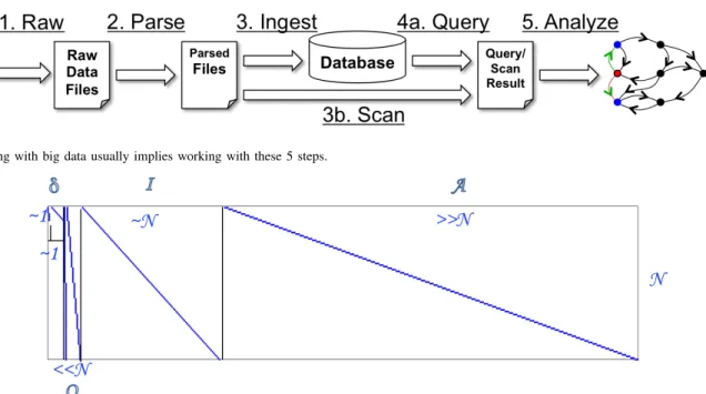
Fig. 1. Working with big data usually implies working with these 5 steps.

Fig. 2. A database can be represented as the sum (concatenation) of a series of sub associative arrays that correspond to different ideal or vestigial arrays

First, it is necessary to define the components of a database in formal terms.

A database can be represented by a model that is described as a sum of sparse associative arrays, Figure 2. Consider a database E represented as the sum of sparse sub-associative arraysEi: E= n

∑

Whereicorresponds to different entities that comprise then entities of E. EachEi has the following properties/definitions:

• N is the number of rows in the whole database (number of rows in associative array E).

• Ni is the number of rows in database entityi with at least one value (number of rows in associative array Ei).

• Miis the number of unique values in database column i(number of columns in associative array Ei).

• Vi is the number of values in database column i (number of non zero values in associative arrayEi). With these definitions, the following global sums hold:

N≤

_∑

_∑

_∑

where N, M, and V correspond to the number of rows, columns and values in database Erespectively.

Theoretically, each sub-associative array (Ei) can be typed as idealorvestigialarrays depending on the properties of this sub-associative array:

• Identity (I): Sub-associative array Ei in which the number of rows and columns are of the same order:

Ni∼Mi

• Authoritative (A): Sub-associative array Ei in which the number of rows is significantly smaller than the number of columns:

NiMi

• Organizational (O): Sub-associative arrayEi in which the number of rows is significantly greater than the number of columns:

NiMi

• Vestigial (δ): Sub-associative array Ei in which the number of rows and columns are significantly small

Ni∼1 Mi∼1

Conceptually, data collection for each of the entities is intended to follow the structure of ideal models. However, due to inconsistencies and changes over time, they may develop vestigial qualities or differ from the intended ideal array. By comparing a given sub associative array to the structures described above, it is possible to learn about a given database and recognize inconsistencies or errors.

A. Performing DDA

Consider a databaseE. In a real system,Eis a large sparse associative array representation of all the data in a database using the schema described in the previous sections. Suppose that Eis made up of kentities, such that:

E=

k

∑

1

In a real database, these entities typically relate to vari-ous dimensions in the dataset. For example, entities may be time stamp, username, building id number, etc. Each of the associative arrays corresponding to Ei is referred to as a sub-associative array. Dimensional analysis compares the structure of each Ei with the intended structural model. This process consists of the steps described in Algorithm 1.

Data: DB represented by sparse associative array E

Result: Dimensions of sub-associative arrays corresponding to entities

forentity i in k do

read sub-associative arrayEi∈E;

ifnumber of rows in Ei≥1 then number of rows inEi =Ni;

number of unique columns inEi=Mi; number of values in Ei=Vi;

else

go to next entity;

end end

Algorithm 1:Dimensional Analysis Algorithm Using the algorithm above, let the dimensions of each sub associative array (Ei) be contained in the 3-tuple (Ni, Mi,Vi) corresponding to the number of rows, columns and values in each sub associative array which corresponds to a single entity. B. Using DDA Results

Once the tuples corresponding to each entity is collected for a database E, one can compare the dimensions with the idealandvestigialarrays described in Section III to determine the approximate intended structural model for each entity.

Once the intended structural model for an entity is deter-mined, it is possible to highlight interesting patterns, anoma-lies, formatting, and inconsistencies. For example:

• Authoritative (A): Important entity values (such as usernames, words, etc.) are highlighted by:

Ei∗1Nx1>1

11xN∗Ei>1

• Identity (I): Misconfigured or non-standard entity val-ues are highlighted by:

Ei∗1Nx1>1

11xN∗Ei>1 INxN−Ei6=0NxN

• Organizational (O): The mapping structure of a sub-associative array is highlighted by counts and corre-lations in which:

Ei∗1Nx11

E_iT∗Ej>>1 11xN∗Ei=1

• Vestigial (δ): Erroneous or misconfigured entries can

typically be determined by inspectingEi.

The difference between a sub-associative array and an in-tended model such as those above provide valuable information about failed processes, corrupted or junk data, non-working

sensors, etc. Further, the actual dimensions of each sub-associative array can provide information about the structure of a database that enables a high level understanding of a particular data dimension.

IV. APPLICATIONEXAMPLES

In this section, we provide two example data sets and the results obtained through DDA. This section is meant to illustrate the concepts described before.

A. Geo Tweets Corpus

Social media analysis is a growing area of interest in the big data community. Very often, large amounts of data is collected through a variety of data generation processes and it is necessary to learn about the low level structural information behind such data. Twitter is a microblog that allow up to 140 character “tweets” by a registered user. Each tweet is published by Twitter and is available via a publicly acessible API. Many tweets contain geo-tagged information if enabled by the user. A prototype twitter dataset containing 2.02 million tweets was used for the dimensional analysis.

1) Dimensional Analysis Procedure: The process outlined in the previous section was used to perform dimensional analysis on a set of Twitter data with the intent of finding any anomalies, special accounts, etc. The database consists of 2.02 million rows and values distributed across 10 different entities such as latitude, longitude, userID, username, etc.

The associative array representation of the Twitter corpus is shown in Figure 3. The 10 dimensions or entities of the database that make up the full dataset are also shown.

2) DDA Results: Dimensional analysis of the dataset can be performed by performing Algorithm 1 on each of the entities (i) inkpossible entities. For example,E7=ETimewhich is the associative array in which all of the column keys cor-respond to time stamps. Thus, the triple (NTime,VTime,MTime) is the number of entries with a time stamp, number of time stamp entries in the corpus, and number of unique time stamp values respectively. Performing Algorithm 1 on each of the 10 entities yields the results described in Table I.

Using the definitions defined in Section III, we can quickly determine important characters. For example, to find the most popular users, we can look at the difference where Euser∗1Nx1>1. Using D4M, this computation can easily be

performed with associative arrays to yield the most popular users. Performing this analysis on the full 2.02 million tweet dataset represented by an associative array E:

% Extract Associative Array Euser

>>Euser = E(:,StartsWith('user|,'));

%Add up count of all users

>>Acommon = sum(Euser, 1);

%Display most common users

>>display(Acommon>150);

(1,user|SFBayRoadAlerts) 258 (1,user|akhbarhurra) 177 (1,user|attir_midzi) 159 (1,user|verkehr_bw) 300

The results above indicate that there are 4 users who have greater than 150 tweets in the dataset.

Fig. 3. Associative Array representation of Twitter data.E1,E2, ...,E10represent the concatenated associative arraysEi that constitute all the entities in the full dataset. Each blue dot corresponds to a value of 1 in the associative array representation.

Entity Ni Vi Mi Structure Type

latlon 1624984 1625197 1506465 Identity lat 1624984 1625192 1504469 Identity lon 1625061 1625725 1504619 Identity place 1741337 1741516 1504619 Identity retweetID 636455 636644 627163 Identity reuserID 720624 722148 676616 Identity time 2020000 2020000 35176 Organization userID 2020000 2020000 1711141 Identity user 2020000 2020000 1711143 Identity word 1976746 17180314 7838862 Authority

TABLE I. DIMENSIONALANALYSIS PERFORMED ON2.02MILLIONTWEETS

50,0000 100,000 200,000 500000 1000000 2000000 500 1000 1500 2000 2500 Number of Tweets

Time for DDA/Data Ingest (seconds)

DDA and Ingestion times for Twitter Data DDA Time

DB Ingest Time

Fig. 4. Relative performance between DDA and ingesting data.

3) DDA Performance: Ingesting data into a database is often an expensive and time consuming process. One of the features of DDA is in the ability to potentially reduce the amount of information that needs to be stored. Figure 4 describes the relative time taken by DDA compared to data ingest.

From this comparison, it is clear that DDA takes a fraction of the time compared to ingest. By using DDA, one may be able to remove entries that need to be ingested, thus reducing the overall ingest time.

B. HPC Scheduler Log Files

Another application in which dimensional analysis was tested is with HPC scheduler log files. LLSuperCloud uses the Grid Engine scheduler for dispatching jobs. For each job that is finished, an accounting record is written to an accounting file. These records can be used in the future to generate statistics about accounts, system usage, etc. Each line in the accounting file represents an individual job that has completed.

1) DDA Procedure: The process outlined in the previous section were used to perform dimensional analysis on a set of SGE accounting data with the intent of finding any anomalies, special accounts, etc. The database consists of approximately 11.5 million entries with 27 entities each. A detailed descrip-tion of the entities in the SGE accounting file can be found at: [11].

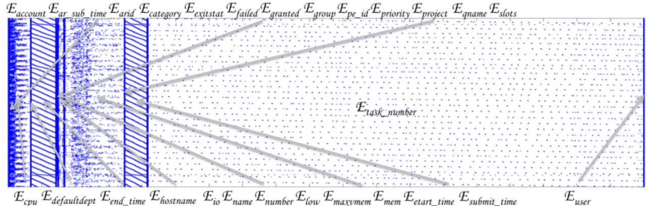
The associative array representation of the SGE corpus is shown in Figure 5. The 27 “dimensions” of data that make up the full data set are shown in figure 5.

2) DDA Results: After performing dimensional analysis on the SGE corpus, the results are tallied for inspection. A subset of the results is shown in Table II. It is interesting to note that there are many accounting file entries that are not collected and have only default values. For example, the field “defaultdepartment” contains only one unique value in the entire dataset - “default”. For an individual wishing to perform more advanced analytics on the dataset, this is an important result and can be used to reduce the dimensionality of each data point.

A D4M code snipped to find the most common job names is shown below.

% Extract Associative Array Euser

Fig. 5. Associative Array representation of SGE accounting data represent the concatenated associative arraysEi that make up the full dataset.

Entity Ni Vi Mi Structure Type

Account 11446187 11446187 1 Vestigial

CPU Hours 11446187 11446187 2752964 Identity Default Department 11446187 11446187 1 Vestigial

Job Name 11446187 11446187 90491 Organization Job Number 11446187 11446187 485212 Identity Memory Usage 11446187 11446187 5241559 Identity

Priority 11446187 11446187 1 Vestigial

Task Number 11446187 11446187 7491889 Identity User Name 11446187 11446187 8388 Organization

TABLE II. DIMENSIONALANALYSIS PERFORMED ON 11.5MILLIONSUNGRIDENGINE ACCOUNTING ENTRIES. ONLY SELECTED ENTRIES ARE SHOWN OF THE27TOTAL ENTRIES COLLECTED

%Add up count of all users

>>Acommon = sum(Ejobname, 1);

%Display most common users

>>display(Acommon>1000000);

(1,job_name|rolling_pipeline.sh) 2762791 (1,job_name|run_blast.sh) 1256422 (1,job_name|run_blast_parser.sh) 1162522

Interestingly, of the 27 dimensions of data in the SGE log files, 8 of the entities are not actually recorded. This infor-mation can be very important to one interested in performing advanced analytics on a dataset in which nearly one third of the data is unchanging.

V. CONCLUSIONS ANDFUTUREWORK

In this paper, we proposed a process to understand the structural characteristics of a database called dimensional data analysis. Using DDA, a researcher can learn a great deal about the hidden patterns, structural characteristics and possible errors of a large unknown database. DDA consists of representing a dataset using associative arrays and performing a comparison between the constituent associative arrays and intended ideal database arrays. Deviations from the intended model can highlight important details or incorrect information. We recommend that the DDA technique be the first step of an analytic pipeline. The common next steps in an analytic pipeline such as background modeling, feature extraction, machine learning and visual analytics depend heavily on the quality of input data.

Next steps to this work include developing an automated mechanism to perform background modeling of big datasets, and application of detection theory to big data sets.

ACKNOWLEDGMENT

The authors would like to thank the LLGrid team at MIT Lincoln Laboratory for their support and expertise in setting up the computing environment.

REFERENCES

[1] D. Laney, “3d data management: Controlling data volume, velocity and variety,”META Group Research Note, vol. 6, 2001.

[2] A. Reuther, J. Kepner, W. Arcand, D. Bestor, B. Bergeron, C. Byun, M. Hubbell, P. Michaleas, J. Mullen, A. Prout,et al., “Llsupercloud: Sharing hpc systems for diverse rapid prototyping,” in High

Perfor-mance Extreme Computing Conference (HPEC), 2013 IEEE, pp. 1–6,

IEEE, 2013.

[3] J. Kepner, W. Arcand, W. Bergeron, N. Bliss, R. Bond, C. Byun, G. Condon, K. Gregson, M. Hubbell, J. Kurz, et al., “Dynamic distributed dimensional data model (d4m) database and computation system,” inAcoustics, Speech and Signal Processing (ICASSP), 2012

IEEE International Conference on, pp. 5349–5352, IEEE, 2012.

[4] E. Bingham and H. Mannila, “Random projection in dimensionality reduction: applications to image and text data,” in Proceedings of the seventh ACM SIGKDD international conference on Knowledge

discovery and data mining, pp. 245–250, ACM, 2001.

[5] P. Indyk and R. Motwani, “Approximate nearest neighbors: towards removing the curse of dimensionality,” inProceedings of the thirtieth

annual ACM symposium on Theory of computing, pp. 604–613, ACM,

1998.

[6] “Apache accumulo,”https://accumulo.apache.org/.

[7] C. Byun, W. Arcand, D. Bestor, B. Bergeron, M. Hubbell, J. Kepner, A. McCabe, P. Michaleas, J. Mullen, D. O’Gwynn, et al., “Driving big data with big compute,” inHigh Performance Extreme Computing

(HPEC), 2012 IEEE Conference on, pp. 1–6, IEEE, 2012.

[8] J. Kepner, C. Anderson, W. Arcand, D. Bestor, B. Bergeron, C. Byun, M. Hubbell, P. Michaleas, J. Mullen, D. O’Gwynn, et al., “D4m 2.0 schema: A general purpose high performance schema for the accu-mulo database,” inHigh Performance Extreme Computing Conference

(HPEC), 2013 IEEE, pp. 1–6, IEEE, 2013.

[9] J. Kepner and J. Gilbert,Graph algorithms in the language of linear algebra, vol. 22. SIAM, 2011.

[10] J. Kepner, D. Ricke, and D. Hutchinson, “Taming biological big data with d4m,”Lincoln Laboratory Journal, vol. 20, no. 1, 2013. [11] “Ubunto manpage: Sun grid engine accounting file format,”