2019_Onderdonk.pdf

(1)

THE EFFECTS OF BOX OFFICE AND HOME ENTERTAINMENT REVENUE PERFORMANCE ON EQUITY VALUATIONS IN THE FILM INDUSTRY

John W. Onderdonk

An honors thesis submitted to the faculty of the Kenan-Flagler Business School at the University of North Carolina at Chapel Hill

Chapel Hill 2019

Approved by_________________________________

(2)

ABSTRACT

John W. Onderdonk

The Effects of Box Office and Home Entertainment Revenue Performance on Equity Valuations in the Film Industry

(Under the direction of Riccardo Colacito, Ph.D.)

The film industry relies on a variety of different revenue streams that contribute to the

overall financial success or failure of film companies. These companies derive the

majority of their revenue from box office and home entertainment sales. The purpose of

this research is to evaluate the effects of box office and home entertainment revenue

performance on the equity valuations of companies in this industry. Using estimation

techniques commonly found in finance literature, this study concludes that box office

performance significantly impacts the equity valuations of film companies over both

short-term and long-term periods. This study also reveals the effects of news on investor

sentiment, demonstrates the cyclicality of company performance in the film industry, and

proposes profitable trading strategies to capitalize on box office performance data. Using

estimation techniques under similar circumstances, this study did not find a significant

(3)

ACKNOWLEDGEMENTS

The successful completion of this thesis was ultimately made possible by the

overwhelming support I have received over the years from far more educators, friends,

and family members than I could possibly list. Thank you all. I would also like to

recognize some specific individuals for their key contributions to the completion of this

work:

• Dr. Riccardo Colacito, Thesis Advisor, for your constant guidance and support

throughout this process. Your passion for education and your commitment to the

success of your students is truly inspiring.

• Dr. Patricia Harms, Proposal Advisor, for your dedication to bringing out the

best in your students and equipping me with the tools necessary to conduct

original research.

• Anonymous data provider, for graciously providing me with the resources

necessary to perform a fundamental component of my analysis. Thank you to all

involved.

Finally, I would like to thank my parents (Todd and Sarah) and my brothers (Colin and

Daniel). You have always encouraged me and motivated me to make the best of every

opportunity, and none of this would have been possible without your loving support all

(4)

LIST OF TABLES

Table 1 Opening Weekend Box Office Returns ...36

Table 2 Box Office Annualized Contemporaneous Returns – 3 Portfolios ...42

Table 3 Box Office Annualized Contemporaneous Returns – 2 Portfolios ...43

Table 4 Box Office Annualized Conditional Returns – 3 Portfolios ...47

Table 5 Box Office Annualized Conditional Returns – 2 Portfolios ...48

Table 6 Home Entertainment Annualized Conditional Returns ...53

Table 7 Box Office / Home Entertainment Correlations ...56

Table 8 One-Month Box Office Annualized Conditional Returns – 3 Portfolios ...59

(7)

LIST OF FIGURES

Figure 1 “Hit”-Minus-“Flop” Portfolio Performance ...30

Figure 2 “Hit” Portfolio Performance ...30

(8)

LITERATURE REVIEW

Introduction

Characterized by perpetual creative destruction, the business world constantly

replaces old technology with new technology to create competitive advantage and adapt

to changing consumer preferences. Established industries and companies within those

industries must match or exceed the innovations of new ventures in order to stay

competitive and maintain market position. The film industry faces similar pressures from

new innovations and competitive threats. Industry disruption due to the widespread

adoption of streaming from companies like Netflix and Hulu has reduced demand for

traditional home entertainment products, such as DVDs and Blu-Ray Discs. This

declining demand for product offerings has prompted film companies to adjust their

product mixes to reduce costs and increase consumer willingness to pay, resulting in

rising profit margins for these companies.1 Given the niche nature of the home

entertainment industry, academic researchers have not explored the joint effect of

declining home entertainment demand and rising profit margins on actual profitability or

investor expectations regarding profitability. Therefore, the joint effect of declining sales

and rising profit margins is currently ambiguous to industry outsiders.

Due to the sparse nature of previously conducted research on the film industry,

(9)

repositories to explain the state of the industry. The estimation techniques that I will use

to demonstrate the relationships between box office revenue, home entertainment sales,

and stock price performance are commonly used in finance academic literature, and I will

chronicle the progression of scholarly research in the field. Through my research, I aim to

use these common finance estimation techniques to yield novel insights in a relatively

unexplored industry.

This review of popular press and academic literature provides an assessment of

relevant information regarding the film industry and finance estimation techniques. In the

following sections, this review will analyze (1) the box office and home entertainment

segments of the broader film industry, (2) innovations and disruptions in the home

entertainment industry, (3) the use of finance estimation techniques to price assets

according to observable characteristics, (4) the role of exogenous factors in asset pricing,

and will include (5) a conclusion to draw connections between the disparate elements of

this literature review.

Box Office and Home Entertainment as Segments of the Film Industry

The film industry is divided into multiple segments that generate revenue for film

companies. Business functions within the film industry include box office,

merchandising, home entertainment, and television licensing. Due to consolidation in the

entertainment industries, large media conglomerates (e.g., Disney, Comcast

NBCUniversal, and Fox) typically own and control each functional segment for the films

they produce and opt to license intellectual property for use in consumer products. This

(10)

domestic film industry, (b) the historical role of home entertainment specifically in the

broader industry, and (c) shortcomings of traditional performance measures.

Additionally, this section will rely somewhat heavily on popular press and online data

repositories due to limited academic research on this industry.

Domestic film industry

The domestic film industry is comprised of a few companies with a broad array of

revenue streams that outsiders typically estimate according to a single metric.

Consolidation within the industry has led to the formation of conglomerates with many

different business units. In the film industry, six major companies made up a combined

77% of box office revenue from 1995 through 2018: Walt Disney Studios, Warner Bros.,

Sony/Columbia Pictures, 20th Century Fox (recently acquired by Disney), Universal

Pictures, and Paramount Pictures (Richter, 2018). Though films generate many ancillary

revenue streams, the public typically judges the success or failure of a film solely by its

opening weekend box office performance (Young, Gong, Stede, Sandino, & Du, 2008, p.

9). This three-day period for a film determines its value from a contractual standpoint

with regard to licensing deals for television, merchandising, streaming, etc. (Young et.

al., 2008, p. 9). Additionally, because of its public availability, industry insiders use this

box office metric as a predictive tool to estimate internal and external performance of

ancillary revenue streams and make business decisions accordingly.2 As Powers (2015)

(11)

revenue assumptions are often unreported, and “investments are not even necessarily

priced by outsiders” (p. 1). Though judging success according to a single metric

seemingly diminishes the importance of a film’s ancillary revenue streams, these

additional sources of revenue make a huge impact on the industry’s bottom line. In 2017,

for instance, domestic box office revenue totaled $10.51B across the industry while home

entertainment sales grossed $20.49B (McCourt, 2018). Despite the apparent materiality

of a film’s diverse array of revenue streams, financial performance in the film industry

continues to face judgment according to a single metric.

Home entertainment segment

The home entertainment segment, though often viewed as secondary to the box

office segment, has a long history of product innovation that demonstrates the importance

of its financial performance to the overall film industry. Home entertainment’s storied

history began in 1977 when Magnetic Video first utilized JVC’s 1976 VHS technology to

release feature-length films that could be viewed at home for $50-75 per copy (Epstein,

2015). The next significant technological advancement took place in 1997 when home

entertainment companies introduced DVD players and discs to provide better picture and

sound quality along with endless reusability (Epstein, 2015). Home entertainment

companies further enhanced this superior picture and sound quality with the release of

Blu-Ray discs in 2006, and Apple eliminated the need for physical media altogether with

its Apple TV streaming service in 2007 (Epstein, 2015). Lionsgate became the first

movie studio to release the latest and most superior home entertainment technology—4K

(12)

offerings today include both digital media (e.g., subscription video-on-demand, digital

purchases, digital rentals) and physical media (e.g., DVD, Blu-Ray, 4K, physical rentals).

Subscription streaming comprises the largest share of the market, followed by physical

media purchases (McCourt, 2018). The film industry has invested significantly in

innovating new home entertainment technologies to provide a better viewing experience

for consumers, which demonstrates the financial importance of the home entertainment

segment to the broader film industry.

Shortcomings of traditional performance measures

As detailed in a previous subsection, film industry analysts place disproportionate

emphasis on box office revenue to evaluate film financial performance despite the

materiality of other industry segments, such as home entertainment. If actual performance

of the film industry’s ancillary revenue streams deviates significantly from the

performance expected from a given film at a given box office level, then the research of

Young et. al. (2008) would suggest analysts might not detect the deviation. According to

the market size statistics from McCourt (2018), this limitation in publicly available

knowledge could cause dramatic misestimation in aggregate financial performance for a

film. Researchers have not yet explored whether or not actual performance from the

ancillary revenue streams of a film directly affects sentiment regarding the financial

(13)

Innovations and Disruptions in Home Entertainment

The home entertainment segment of the film industry has changed dramatically

since its advent in 1977 due to technological innovations and disruptions to the industry.

Two significant disruptions affected the way in which customers view media in the home.

In 1985, Blockbuster opened its first store in Dallas, TX, allowing customers to rent

physical media for brief periods of time to watch and return (Epstein, 2015). In 2007,

Netflix started streaming movies online, which allowed consumers to watch movies

instantly with no physical media required (Rodriguez, 2017). Both of these disruptions

strongly affected home entertainment companies and forced them to adapt their business

models to survive in the new environment.

Blockbuster’s rental disruption

In 1985, Blockbuster started siphoning revenues from film companies through its

rental system that disincentivized the purchase of home entertainment products.

Customers who only wanted to watch a movie once after its theatrical release could do so

at a much lower cost than purchasing the movie outright. Instead of fighting this trend,

film companies saw the disruptive force of Blockbuster as an opportunity to generate

revenue from price-sensitive customers who would be willing to pay for a rental but not

for a purchase. They entered into strategic revenue-sharing alliances in which they sold

movies in bulk to Blockbuster at a discount and collected a percentage of rental revenues,

which ultimately generated higher sales for both Blockbuster and the film companies

(Carr, Muthsamy, & Owens, 2012, p. 69). Through these partnerships, home

(14)

industry disruption. Though Blockbuster eventually declared bankruptcy due to the

significant decline in physical rental (McCourt, 2018), Family Video, one of

Blockbuster’s competitors, has maintained a thriving rental business with over 700 stores

by creating a fun, family-friendly shopping experience and servicing areas of the country

without high-speed internet (Fink, 2018).

Netflix’s streaming disruption

With the advent of Netflix’s streaming service in 2007, home entertainment faces

a threat to physical media altogether. Like the traditional film industry, subscription

streaming is a highly concentrated industry dominated by a few large competitors. Netflix

leads the industry with 74% U.S. household penetration in 2018, followed by Hulu and

Amazon with 36% and 28% penetration, respectively (Engleson, 2018). In 2017, $9.55B

of domestic home entertainment revenue came from subscription streaming, increasing

31% from 2016 (McCourt, 2018). DVD and Blu-Ray sales, on the other hand, accounted

for only $4.72B, decreasing 14% from 2016 (McCourt, 2018). Home entertainment

companies obtain payments to license content to streaming services, but this source of

revenue has swiftly undercut physical media consumption (Hilderbrand, 2010, p. 27-28).

As with the competitive challenge Blockbuster presented in 1985, film companies

are trying to adapt their business models to survive in a world dominated by subscription

streaming and with physical media usage in sharp decline. Though physical unit sales are

(15)

which has lowered the cost-per-unit due to the lack of production and distribution costs

associated with digital media. They have also promoted higher-priced, higher-margin

physical media formats, such as Blu-Ray and 4K Ultra HD, by demonstrating the

enhanced sound and picture quality of those formats relative to subscription streaming.3

Film companies, thus, take a multi-pronged approach to maintaining profitability despite

the rapid adoption of subscription streaming. However, no published research exists

regarding how revenue fluctuations in the home entertainment industry affect investor

sentiments regarding profitability. As discussed previously, the lack of publicly available

sales information leads to the overemphasis of box office performance to indicate

financial performance for films.

The Use of Finance Estimation Techniques to Price Assets

This section of the Literature Review will detail the development of prominent

asset pricing techniques that estimate returns according to observable characteristics.

Investors and finance professionals have attempted to price companies according to

observable characteristics for decades by finding significant relationships between

company characteristics and stock price movement. In contrast with the previous two

sections of this literature review, the academic literature on asset pricing models and

finance estimation techniques is extensive. This section will explore (a) the development

of prominent asset pricing models, (b) an example of the process for identifying an

additional significant factor, and (c) the purpose of finance estimation techniques.

(16)

Development of prominent asset pricing models

Asset pricing models seek to estimate returns to a given financial instrument

based on one or more factors. Jensen, Black, & Scholes (1972) put forth the first

generally accepted asset pricing model—called the Capital Asset Pricing Model

(CAPM)—that attempts to value securities as a function of their “systematic,” or

“market,” risk. The model only accounts for systematic risk in determining the price of a

security because they assumed that idiosyncratic risk can be removed through a

well-diversified portfolio. The fundamental finding of the model is that the beta of a stock—

which is the covariance of the returns of that stock with the return of the market divided

by the variance of the market—determines the risk premium of the stock. As beta

increases, the expected return of the stock increases. Subsequent researchers found that a

single-factor model that only considers market risk does not capture risk factors that

would be evident in a multi-factor model.

Fama & French (1992) critiqued the research of Jensen, Black, & Scholes,

arguing that the simple relationship between an asset’s beta and its average return

disappears with more recent data from 1963 to 1990. They do not support the finding that

average stock returns are positively related to market beta. Instead, they argue that, in the

period from 1963 to 1990, a firm’s size and book-to-market equity “capture the

cross-sectional variation in average stock returns associated with size, E/P, book-to-market

equity, and leverage” (p. 450). These two factors can be used as a proxy for risk in

(17)

market excess return, (2) return on small-cap stocks minus return on large-cap stocks, and

(3) return on value stocks minus return on growth stocks. The resulting three-factor

model explains excess returns on a cross-section of stocks that would be viewed as

abnormal by the research of Jensen, Black, & Scholes. Fama & French (1993) essentially

expanded on the work of Jensen, Black, & Scholes by adding two additional factors to

make the asset pricing model more robust.

Example of the process for identifying an additional statistically significant factor

After Fama & French (1993) created a multifactor asset pricing model,

subsequent researchers sought to improve the model further by adding additional factors.

Jegadeesh & Titman (1993) examined the role that “momentum” plays in generating

excess returns for stocks, finding that previous “winners” in the market exhibit a

statistical tendency to become future “winners.” Grinblatt, Titman, & Wermers (1995)

affirm this research by demonstrating that mutual funds following momentum strategies

exhibit excess returns over time. Carhart (1997) constructed a “4-factor model using

Fama and French's (1993) 3-factor model plus an additional factor capturing Jegadeesh

and Titman's one-year momentum anomaly” (p. 61) to create a more robust four-factor

model. In light of new research, Fama & French (1996) examined their original

three-factor model and concluded that their model failed to account for excess returns due to

momentum. Researchers during this time typically viewed momentum as a relevant factor

driving returns exclusively at the individual security level. Moskowitz & Grinblatt

(1999), on the other hand, argued that momentum strategies for individual stocks become

(18)

reside. In other words, industry momentum almost entirely explains the momentum effect

at the individual security level. The identification of momentum and further debate

regarding its role in explaining asset return anomalies illustrate that new observable

characteristics can be combined with previously accepted factors in an attempt to

estimate asset returns.

Purpose of estimation techniques

The substantial amount of research in finance literature regarding momentum and

other factors in asset pricing models demonstrates that stock returns can be estimated

according to observable characteristics. Estimation techniques like those of Fama &

French (1992) can demonstrate whether or not a significant relationship exists between a

given observable characteristic and fluctuations in stock price. As evidenced by the

evolution of asset pricing models through the decades, prominent researchers constantly

use estimation techniques to look for new observable characteristics that affect stock

prices, and they often disagree about the most predictive asset pricing models.

The Role of Exogenous Factors in Asset Pricing

Researchers have explored the effects of observable characteristics on asset prices

to a great extent. Most of these observable characteristics are financial metrics specific to

given companies, such as size, valuation, recent performance, etc. However,

(19)

The role of demand shocks in affecting asset prices

Demand shocks are sudden events that increase or decrease a consumer’s desire

for a particular good or service in the market. One example of a negative demand shock

is the reduction in demand for physical media as a result of Netflix’s entry into digital

streaming in 2007. Lucas (1978) presented an asset pricing model that placed the equity

premiums of assets on the supply side of the economy while assuming consumption

demand to have no volatility. Bansal & Yaron (2004) rebutted this model, arguing that

consumption demand is also stochastic (subject to shocks), and it arguably plays a more

integral role in determining the equity premium of an asset. Continuing the line of

thinking of Bansal & Yaron (2004), Albuquerque, Eichenbaum, Luo, & Rebelo (2016)

argue that the fact that conventional asset pricing models place all uncertainty onto the

supply side of the economy while neglecting demand uncertainty creates a weak

correlation between stock returns and observable fundamentals. They ascribe the majority

of the equity premium to demand shocks. Recent research indicates that exogenous

demand shocks affect the risk premium associated with a stock and, therefore, its price.

The role of news events in affecting asset prices

Significant news events or coverage also affect asset prices. Engle & Ng (1993)

explore the relationship of news—good or bad—to asset price volatility. Though none of

their models perfectly capture the asymmetrical effect of new information on stock price

volatility, their study found conclusively that negative news coverage affects volatility

with greater magnitude than positive news coverage. Furthering this research on the

(20)

increase in Google search volume predicts higher stock prices in the next two weeks as

the market absorbs new information followed by an eventual stock price reversal within a

year. Their study of search volume also indicated strong first-day performance and

long-term underperformance of a sample of IPO stocks. These studies show that news

powerfully affects stock prices for extended periods of time after the initial coverage as

the market incorporates new information.

Innovations affecting asset prices

Economists have recently found that levels of innovation can be measured and

demonstrated to affect asset prices. Kogan, Papanikolaou, Seru, & Stoffman (2017)

explored the role that technological innovation plays in spurring economic growth. In

their research methodology, they use newly collected data on patents issued to U.S. firms

from 1926 to 2010 as a proxy for technological innovation, and, expanding on the work

of Engle & Ng (1993), they compare stock price responses to patent news as a means to

show the effect of patents on economic growth. Kogan et. al. found that innovation “is

associated with substantial growth, reallocation, and creative destruction” (p. 706). They

discovered a significant relationship between patents (as a proxy for innovation) and

stock prices as a proxy for firm growth. As a result, they conclude that technological

innovation accounts for significant medium-run fluctuations in aggregate economic

growth. This research and the research in the prior subsections demonstrate that

(21)

Conclusion

The domestic home entertainment industry is a large, multi-billion-dollar segment

of the broader domestic film industry. Due to the use of traditional industry performance

metrics, such as box office revenue, and the lack of publicly available data on home

entertainment sales, analysts estimate the performance of home entertainment and other

ancillary revenue streams for a given film largely based on opening weekend box office

revenue. The inability of this metric to provide accurate estimates could severely misstate

the aggregate financial performance of a film because of the sizable percentage of

revenue coming from outside the box office.

Due to industry disruption through streaming, the market for home entertainment

has experienced a negative demand shock. The popular press has documented these

industry changes extensively, and home entertainment companies have introduced new

innovations to increase retail prices, cut costs, and maintain increasing profitability.

According to the academic research documented in this literature review, the stock prices

of home entertainment companies should theoretically fluctuate as a result of these

changes to the industry. However, the use of box office performance as a proxy for

aggregate film performance potentially obscures the actual fluctuations in demand and

profitability resulting from these industry changes.

Finance estimation techniques, as detailed in this literature review, can indicate

whether a significant relationship exists between box office revenue or home

entertainment sales and the stock price performance of film companies. In the context of

finance literature, box office revenue and home entertainment sales represent “observable

(22)

determine whether or not a relationship exists. A lack of a significant relationship

between home entertainment sales and stock returns could potentially indicate the

ineffectiveness of using box office performance as the sole performance metric for a film

because home entertainment sales do directly affect profitability and should, therefore,

affect stock prices. The relationships between box office revenue, home entertainment

sales, and the stock price performance of film companies have not been investigated

(23)

DATASET OVERVIEW

Introduction

In this section, I detail the specifics of datasets that I use to demonstrate the

effects of box office performance and home entertainment performance on the equity

valuations of film companies. To determine the effects of box office and home

entertainment performance on film company stock prices, I use (a) historical stock price

data, (b) historical box office revenue data, and (c) historical home entertainment revenue

data. I detail the sources and specifics of these datasets in the following section.

Historical Stock Price Data

In this study, I use historical stock price data from May 2001 through November

2018. My dataset contains daily opening prices and daily closing prices adjusted for

dividend payments spanning that duration. Most stock price data used in this study comes

from S&P Capital IQ, which I used as the default source for my price data. However,

some companies from 2001 through 2018 have undergone mergers that resulted in the

de-listing of the companies from exchanges. Though S&P Capital IQ can pull historical data

from companies that currently exist, it cannot retrieve data from companies, such as Time

Warner, that have recently been acquired and are no longer listed on an exchange. In such

instances, I used Investing.com because they publish records of historical data on

(24)

Historical Box Office Performance Data

I use Box Office Mojo as the source of my box office data. Box Office Mojo is

often used by industry insiders due to the reliability of its data reporting.4 For Section 1,

which examines the stock returns of box office “hits” versus box office “flops” as defined

by opening weekend performance, I use their datasets “Biggest Opening Weekends”

(+$50M) and “Worst Openings” (3,000+ theaters), which yield data on 235 films and 200

films, respectively. These openings were adjusted to 2019 dollars prior to being ranked.

In Section 2, which examines box office revenues on a monthly basis by

company, I use Box Office Mojo once again based on their monthly year-to-date (YTD)

box office revenue numbers by company. I manually converted these monthly YTD

revenue numbers to monthly revenue numbers (e.g., by subtracting January YTD from

February YTD, etc.) before performing analysis.

Historical Home Entertainment Performance Data

My home entertainment dataset comes courtesy of a data analysis group that

graciously provided me with their dataset free of charge for exclusive use in this research

paper. For the protection of their data, they wish to remain anonymous. The dataset

includes home entertainment revenue by week for seven major film companies dating

back to January 2011. For the purpose of this study and of an equitable comparison with

box office performance, I aggregated the home entertainment data from weekly sales into

(25)

RESEARCH METHODOLOGY

Introduction

The purpose of this section is to outline the methods that I will employ to answer

the following research question: How do box office and home entertainment revenue

performance affect the equity valuations of film companies? Because the following

methodology references industry- and finance-specific terminology that may not be

familiar to all readers, grasping the following list of terms and their definitions is crucial

to understanding both the research methodology and the outcome of the study:

• Box Office: A channel through which media is consumed during its theatrical

release.

• Durbin-WatsonStatistic: A test for autocorrelation in the residuals of a regression.

• Home Entertainment: A channel through which media is consumed

following its theatrical release. Home entertainment for the purpose of this

study involves all associated revenue streams (i.e., purchase, rental,

streaming).

• Factor Portfolio: A portfolio of stocks formed by sorting companies

according to a given observable characteristic (or factor).

• Rebalancing: The re-sorting of factor portfolios according to the given

observable characteristic at a specified time interval.

(26)

• Public Data: Data that is easily accessible and available free of charge to

the public.

• Serial Correlation (Autocorrelation): Correlation between a given variable

and a lagged version of itself. The standard errors must be adjusted to

compensate for the existence of serial correlation in regression.

• Sharpe Ratio: The return of an asset above the risk-free rate over a

specified period divided by the standard deviation in returns over that

same period.

𝑆ℎ𝑎𝑟𝑝𝑒 𝑅𝑎𝑡𝑖𝑜 = 𝑅𝑖 − 𝑅𝑓 𝜎_𝑖

• Significance: A finding that the effect of a given variable is unlikely to

have been zero with 90%, 95%, or 99% confidence.

To answer this study’s research question most effectively, I will (1) examine the

changes in stock prices of companies that released films with the best and worst opening

weekend performances of all time in the days immediately following release and (2)

construct factor portfolios to examine the effects that overperformance and

underperformance in both box office and home entertainment revenue have on the equity

valuations of film companies under different circumstances and periods of time.

(27)

Office Mojo on the films that had the best and worst domestic openings in history.

This methodology will reveal the extent to which opening weekend box office

performance impacts investor expectations for company profitability. The

following subsections will detail (a) the reasoning behind this methodology

selection, (b) an overview of the methodology, and (c) objectives for the

methodology.

Reasoning behind methodology selection

This approach will reveal how investors react in response to “news

events” pertaining to box office performance. According to Box Office Mojo,

when a film is released, box office estimates for the weekend are provided by the

film studios as early as Sunday morning on the weekend of release. The

difference in stock price between the Friday Close and the Monday Open of a

company that just released a smash success “hit” film, or a catastrophically

poor-performing “flop” film, could likely be attributed to changes in market

expectations regarding the performance of that film. By showing how the stock

prices of these companies move in the first two weeks of release, I can

demonstrate how investor expectations regarding the profitability of these film

companies change in a predictable manner in the cycle of each film release.

Overview of the methodology

In this methodology, I will use two sets of quantitative data as outlined in

(28)

stock price data. For both the box office “hits” data and the box office “flops”

data, I will calculate the stock price return of each company in the first 13 days of

release for each given film. “Day 2” will denote the return from Friday Close to

Monday Open on the first weekend of release, and “Day 8” will denote the return

from Friday Close to Monday Open on the second weekend of release. All other

days will denote the returns of the stocks from open to close on standard

weekdays. The average annual return for each day of release will be calculated as

a simple sum of the total returns for each category divided by the number of years

in the sample. Additionally, I will construct a “Hit”-Minus-“Flop” (HMF)

portfolio that holds the stocks of the “hit” releases and shorts the stocks of the

“flop” releases. Based on the results of these portfolios, I will highlight potential

trading strategies that could be implemented to yield profitable outcomes for

investors. These trading strategies will be evaluated based on their historical

Sharpe Ratios, and I will use the average 3-Month Treasury Constant Maturity

Rate from the St. Louis FRED over the sample period as the “risk-free rate of

return.”

One limitation of this methodology is that, based on my criteria for

defining “hits” and “flops,” each calendar year has relatively few titles being

released in those categories. Until 2012, the annual returns for the “flop” portfolio

were particularly erratic due to the relatively few “flop” films being released per

(29)

the dataset in this regard, my analysis in total includes 115 “hit” films and 125

“flop” films.

Finally, I will calculate the standard errors for the returns on each day of

release to determine significance at confidence levels of 90%, 95%, and 99%.

This exercise will differentiate the significant portfolio returns from those not

distinguishable from zero.

Objectives of the methodology

Through this methodology, I will seek to determine how the news of

extreme overperformance or underperformance at the box office affects the stock

prices of film companies in the immediate days following release. This

methodology will demonstrate the degree to which investors pay attention to box

office reports and whether the market incorporates this news into equity

valuations of film companies. Additionally, by constructing the HMF portfolio, I

will be able to better distinguish the returns that are specifically due to box office

performance from returns due to irrelevant factors affecting the stock prices in the

industry. Finally, I hope to use this methodology to propose profitable trading

strategies that investors could employ based on box office data in the days

following the release of a new “hit” or “flop” film.

Research Method 2: Box Office and Home Entertainment Factor Portfolios

In Research Sections 2, 3, and 4 of this paper, I will construct factor portfolios

(30)

periods. With this methodology, I will be using three quantitative datasets. In Sections 2

and 4, which deal exclusively with box office performance, I will use publicly available

box office performance data by studio and by month from Box Office Mojo, and I will

use historical stock price data. In Section 3, which deals exclusively with home

entertainment performance, I will use a proprietary home entertainment dataset from an

anonymous data provider as well as historical stock price data. The following subsections

will detail (a) the reasoning behind this methodology selection, (b) an overview of the

methodology, and (c) objectives for the methodology.

Reasoning behind methodology selection

I will construct these factor portfolios in a similar fashion to those

constructed by Fama & French (1993). With regard to box office revenue

performance, constructing factor portfolios using total box office revenue will

allow me to determine how over- and underperformance for the entire slate of a

given studio affects investor expectations for profitability over varied periods of

time. This approach will lead to a more comprehensive analysis of holistic

company performance than the examination of select films on opening weekend

as in Research Section 1. Constructing factor portfolios in a similar fashion with

home entertainment revenue will allow me to compare the effects of box office

revenue on investor sentiment to the effects of home entertainment revenue on

(31)

volatility. In short, generating factor portfolios that are sorted according to an

observable characteristic will yield insights regarding the effect of that

characteristic on the equity valuations of the underlying companies over time.

Overview of the methodology

The approaches for the methodologies concerning box office revenues and

home entertainment revenues will be similar in many ways with only a few

differences. In both cases, I will develop factor portfolios sorted by

year-over-year (YoY) percentage change in revenue for the respective sorting period. The

justification for sorting according to YoY percentage change as opposed to

percentage change from the previous period is that the film industry features

strong seasonal cyclicality in revenues, meaning that YoY percentage change

would be a more appropriate performance comparison metric. I will examine

sorting period lengths of one, three, six, and 12 months in both the box office and

home entertainment revenue factor portfolios. The “top” portfolio in each instance

will include the top two or top three companies as judged by YoY percentage

change in revenue, and the “bottom” portfolio in each instance will include the

bottom two or three companies as judged by YoY percentage change in revenue.

In tables using only two companies in each portfolio, I will include a “mid”

portfolio containing the returns from all of the companies in between the two

extremes. These portfolios will be rebalanced on a monthly basis according to the

(32)

In addition to the varied lengths in sorting periods, I will also vary the

lengths and starting points of the portfolio holding periods, which will determine

the periods for return calculations. In all cases, I will examine the holding period

returns both contemporaneously with the sorting period and conditionally

according to the sorting from the prior period. Additionally, I will examine

holding period lengths that directly match the sorting period lengths (i.e., one,

three, six, and 12 months), and I will examine holding period lengths of one

month regardless of the sorting period length. I will undertake these factor

portfolio constructions identically for both box office and home entertainment

revenues, though I will withhold certain results due to universally insignificant

findings for particular criteria.

Key differences in the methodologies of the box office revenue and home

entertainment revenue sections emerge from differences in the datasets. The Box

Office Mojo dataset contains data from May 2001 through November 2018, and,

due to changing industry dynamics, features between seven and 12 publicly traded

companies in each period. The proprietary home entertainment dataset, on the

other hand, contains data from January 2011 through November 2018 with a

constant level of seven publicly traded companies per period. One key difference

in the construction of the factor portfolios is that the “mid” portfolio will contain a

varied number of companies in each period for box office performance compared

(33)

lower standard errors of returns relative to those of the home entertainment factor

portfolios, ceteris paribus.

One concern regarding the factor portfolio methodology—in which

holding periods sometimes span multiple months, but returns are reported on a

monthly basis—is the introduction of serial correlation. In instances where the

Durbin-Watson statistics for the returns of factor portfolios indicate the presence

of serial correlation, I will provide heteroskedasticity-adjusted standard errors

using Stata’s “newey” command and a lag value of ⌈ √# 𝑜𝑏𝑠𝑒𝑟𝑣𝑎𝑡𝑖𝑜𝑛𝑠3 ⌉. These

adjusted standard errors will be used to determine significance of returns at

confidence levels of 90%, 95%, and 99%.

Objectives of the methodology

The primary objective of this methodology that I will employ in Research

Sections 2, 3, and 4 is to determine the effect of total box office and home

entertainment revenue performance on equity valuations of film companies over

varied periods. By constructing factor portfolios, I will be able to distinguish the

excess returns due to box office and home entertainment performance from

returns due to extraneous factors affecting the stock prices in the industry.

Additionally, this approach will be more comprehensive in including films other

than the extreme “hits” and “flops” for each company than the approach taken in

Research Section 1. Furthermore, by examining the sorting periods and returns

over longer periods, we can observe any cyclicality emerging from the film

(34)

subsequent periods. Finally, through this methodology, I hope to highlight

profitable trading strategies that investors can employ to capitalize on over- and

(35)

RESEARCH

Introduction

The following sections detail the research that I performed in order to understand

how changes in film industry revenue and news updates affect investor expectations for

profitability of the underlying companies. Section 1 explores the roles that opening

weekend box office “hits” and box office “flops” have on the stock prices of the film

companies that released them. This section will demonstrate that positive and negative

news shocks pertaining to the core film business affect investor sentiment. In Section 2, I

similarly examine box office revenues, but I construct factor portfolios that sort film

companies based on box office performance over longer periods of time. This second

section showcases the ways in which box office performance affects the stock prices of

film companies, and it also reveals the cyclicality of performance in the industry. In

Section 3, I construct identical factor portfolios using home entertainment revenue

instead of box office revenue. This third section demonstrates that home entertainment

performance does not significantly affect investor sentiment or correlate with box office

performance, corroborating both the cyclicality of the industry and the notion that

industry outsiders place disproportionate emphasis on box office revenue as a metric for

performance. Finally, Section 4 includes alternative investment strategies using factor

(36)

Section 1: Stock Price Performance of Opening Weekend “Hits” vs. “Flops”

Overview

In this section, I examine the effects that positive and negative news events have

on investor expectations for profitability. According to Box Office Mojo, opening

weekend box office performance is a metric that is reported for wide-release films on

Sunday mornings between 9:00am and 10:00am PST on the weekend of the film’s

release. The studios provide estimated Friday and Saturday box office revenues with a

projection for Sunday’s revenues. On the Monday following opening weekend, the

studios report actual weekend box office revenues at 1:00pm PST. Studios also report

box office revenue in the first week on the second Friday of release. This information is

publicly available and easily accessible, leading to changes in stock prices for companies

whose films overperform or underperform at the box office.

I aggregated the daily stock price returns following the release of a new film for

two distinct sets of films from 2012 through 2018:

1. Wide-release films in the highest 235 opening weekend box office revenue

performances of all time

2. Wide-release films in the lowest 200 opening weekend box office revenue

performances of all time

In this section, I examine stock price performance in the days following release for the

best- and worst-performing films of all time, and I propose trading strategies that could

(37)

Figure 1 “Hit”-Minus-“Flop” Portfolio Performance

Figure 2 “Hit” Portfolio Performance

Figure 3 “Flop” Portfolio Performance

-10.00% -5.00% 0.00% 5.00% 10.00% 15.00%

1 2 3 4 5 6 7 8 9 10 11 12 13

A v era g e D a il y R eturn

Day of Release

Stock Returns of "Hit"-Minus-"Flop" Portfolio

-8.00% -6.00% -4.00% -2.00% 0.00% 2.00% 4.00% 6.00% 8.00%

1 2 3 4 5 6 7 8 9 10 11 12 13

A v era g e D a il y R etur n

Day of Release Stock Returns of Box Office "Hits"

-8.00% -6.00% -4.00% -2.00% 0.00% 2.00% 4.00% 6.00% 8.00%

1 2 3 4 5 6 7 8 9 10 11 12 13

A v era g e D a il y R eturn

Day of Release Stock Returns of Box Office "Flops"

0.00% 10.00% 20.00% 30.00% 40.00% 50.00% 60.00% 70.00% 80.00% 90.00% 100.00%

FRI MON am MON pm TUES WED THURS FRI MON am MON pm TUES WED THURS FRI

0.00% 10.00% 20.00% 30.00% 40.00% 50.00% 60.00% 70.00% 80.00% 90.00% 100.00%

(38)

Stock price performance of opening weekend “hits”

In first thirteen days following the release of a film with an opening weekend box

office performance in the top 235 of all time by total gross revenue, the companies

releasing the film experience positive stock price returns at two different points in time.

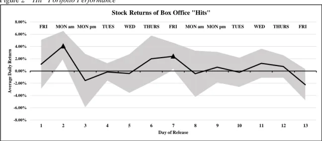
Figure 2tracks the average annualized stock price performance of these box office “hits”

in the first thirteen days of release (“average daily return” in Figure 2). The companies

releasing these films first experience an average annual stock return of 4.09% from the

Friday Close to the Monday Open on the first weekend of release. During this time

period, on Sunday morning, movie studios release projected total weekend box office

revenue. The market has already incorporated this information by the time the weekend

ends, and the aggregate Monday return is indistinguishable from zero. Equivalently,

investors waiting for the official weekend totals on Monday afternoon are likely too late

to capitalize on the positive news effect for that weekend. The second instance of positive

returns occurs on the Friday after opening weekend, which coincides with the release of

the first week’s total box office revenue. The stock prices of these companies rise by an

average of 2.41% annually on this Friday. Returns in the second week after a film’s

release are not significant.

The market is sensitive to the positive performance of high-grossing films during

the early stages of release. However, the stock price in the first two weeks of release only

reflects the positive performance of the films at specific times when new information

(39)

information as the positive news of the good performance of these films becomes widely

available.

Stock price performance of opening weekend “flops”

In first thirteen days following the release of a film with an opening weekend box

office performance in the bottom 200 of all time by total gross revenue, the companies

releasing the film experience a negative stock return at two points in time and a positive

stock return at one point in time. Figure 3tracks the aggregate stock price performance of

these box office “flops” in the first thirteen days of release. The stock price returns

through the first week of release for the companies that produce these films remain

unchanged as a result of their poor performance during the first week. These companies

then experience an average annual return of -1.88% on the second weekend of release

(Friday Close to Monday Open) and an average annual return of -1.73% on the second

Monday of release. These companies likely experience a delay in the negative returns

from their underperformance because negative box office underperformance news is

disseminated much less widely than positive box office overperformance news. Market

participants, and people in general, are likely to be more immediately aware of the

movies that are succeeding at the box office than they are of the movies that are failing.

Because the research of Engle & Ng (1993) would predict that negative news of box

office “flops” would affect the returns with greater magnitude than the positive news of

the box office “hits,” it is fair to assume that the films performing poorly at the box office

had a limited marketing campaign, did not generate social media engagement, and, as a

(40)

in negative returns is that box office “flops” earn a higher percentage of their total

revenue in opening weekend (34%) than box office “hits” (31%). As such,

underperformance in the first weekend suggests even more dramatic underperformance in

subsequent weekends. Investors hoping for a second-weekend rebound in revenue

performance will likely find the opposite effect.

Interestingly, companies that released movies performing in the bottom 200 of all

time by total gross revenue in the opening weekend experience an average annual return

in their stock price of 3.53% on the Thursday in the second week of release. A potential

explanation for this resurgence in stock price is that the production companies could be

“cutting their losses” and removing the movies from the theaters in order to reduce their

costs. The minimum contractually-agreed theatrical run for most movies is two weeks,

and movies that do not make it to the third weekend are typically losing money for the

studios and the theaters by the time they are pulled. A strong positive correlation exists

between box office revenue and theatrical run length (Fahey, 2015), and a movie being

removed from theaters after only two weeks could be seen by investors as a prudent

financial decision on the part of the film companies to minimize their losses.

Additionally, due to the cyclicality of revenues in the film industry, it could be the case

that film companies releasing weaker films will have a natural propensity to release a

stronger film in the following two weeks, which could in part explain the positive returns.

In summary, the market appears to be less immediately and consistently sensitive

(41)

due to the lesser news volume emerging from underperforming films. It appears that

these films in the first weekend of release get ignored by both investors and theatergoers

alike, but investors seem to take note in the second week of release, leading to an initial

decline in stock prices followed by a late-week resurgence potentially due to stop-loss

decision making on the part of the film company and/or due to the release of

higher-caliber films.

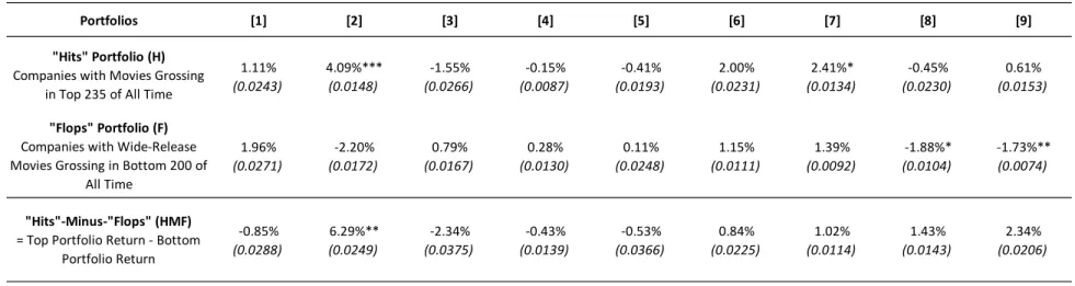
Stock price performance of “Hit”-Minus-“Flop” Portfolio

Figure 1 shows the returns of a hypothetical “Hit”-Minus-“Flop” (HMF) portfolio

that holds the stocks of the companies that had releases in the top 235 opening weekend

box office performances of all time while shorting the companies that had releases in the

bottom 200 of all time, subtracting the returns of the poor performers from the high

performers. In the first thirteen days of release for each given film, this portfolio features

positive returns on one day and negative returns on one day with the rest of the days

having returns statistically indistinguishable from zero. From Friday Close to Monday

Open on opening weekend, this portfolio returns an average of 6.29% annually. As

previously mentioned, film studios release opening weekend projections on Sunday

morning, which is during this period of high return. The market incorporates this news

into the prices of these stocks by the open on Monday, meaning that a portfolio waiting

for the release of the official box office numbers on Monday to employ such a strategy

would be too late and miss the spike in returns.

The HMF portfolio features negative returns on the Thursday in the second week

(42)

the HMF portfolio features an average annual return of -2.81%, which could indicate that

investors assume the strong performance from the “hits” is already “priced in” to the

company’s valuation while the market could have had an overreaction to the “flop” films,

creating an attractive buying opportunity, especially if the companies minimize their

losses by pulling the films from theaters. The key takeaway from the HMF portfolio is

that the market pays close attention to the opening weekend performances of wide-release

films and swiftly incorporates that information into the valuations of the respective

production companies. This example also illustrates the quickness with which news that

is not explicitly associated with a quarterly update or formal financial report can affect

(43)

36

Table 1 Opening Weekend Box Office Returns

Opening Weekend Box Office Returns

(Average Annual Returns from January 2012 through December 2018)

Portfolios [1] [2] [3] [4] [5] [6] [7] [8] [9]

1.11% 4.09%*** -1.55% -0.15% -0.41% 2.00% 2.41%* -0.45% 0.61%

(0.0243) (0.0148) (0.0266) (0.0087) (0.0193) (0.0231) (0.0134) (0.0230) (0.0153)

1.96% -2.20% 0.79% 0.28% 0.11% 1.15% 1.39% -1.88%* -1.73%**

(0.0271) (0.0172) (0.0167) (0.0130) (0.0248) (0.0111) (0.0092) (0.0104) (0.0074)

-0.85% 6.29%** -2.34% -0.43% -0.53% 0.84% 1.02% 1.43% 2.34%

(0.0288) (0.0249) (0.0375) (0.0139) (0.0366) (0.0225) (0.0114) (0.0143) (0.0206)

[1] = This column features average annual returns from Friday Open to Friday Close on the first day of release with the standard errors of the returns in parenthesis below. [2] = This column features average annual returns from Friday Close to Monday Open on the first weekend of release with the standard errors of the returns in parenthesis below. [3] = This column features average annual returns from Monday Open to Monday Close on the first day after opening weekend with the standard errors of the returns in parenthesis below. [4] = This column features average annual returns from Tuesday Open to Tuesday Close on the second day after opening weekend with the standard errors of the returns in parenthesis below. [5] = This column features average annual returns from Wednesday Open to Wednesday Close on the third day after opening weekend with the standard errors of the returns in parenthesis below. [6] = This column features average annual returns from Thursday Open to Thursday Close on the fourth day after opening weekend with the standard errors of the returns in parenthesis below. [7] = This column features average annual returns from Friday Open to Friday Close on the fifth day after opening weekend with the standard errors of the returns in parenthesis below. [8] = This column features average annual returns from Friday Close to Monday Open on the second weekend of release with the standard errors of the returns in parenthesis below.

[9] = This column features average annual returns from Monday Open to Monday Close on the first day after the second weekend of release with standard errors of the returns in parenthesis below.

*, **, and *** denote statistical significance at the 90%, 95%, and 99% levels, respectively.

"Hits" Portfolio(H)

Companies with Movies Grossing in Top 235 of All Time

"Flops" Portfolio (F)

Companies with Wide-Release Movies Grossing in Bottom 200 of

All Time

"Hits"-Minus-"Flops" (HMF)

= Top Portfolio Return - Bottom Portfolio Return

(44)

Potential trading strategies from opening weekend box office performance

Multiple profitable trading strategies emerge from this analysis of opening

weekend box office returns featured in Table 1, including potential for long-only

strategies, short-only strategies, and long-short strategies. Three examples of strategies

that provide high risk-adjusted returns are (1) holding stocks of companies that release

movies in the top 235 from Friday Close to Monday Open on opening weekend, (2)

holding stocks of companies that release movies in the top 235 while shorting stocks of

companies that release movies in the bottom 200 from Friday Close to Monday Open on

opening weekend, and (3) holding stocks of companies that release movies in the top 235

from Friday Close to Monday Open on opening weekend while shorting stocks of

companies that release movies in the bottom 200 from Friday Close to Monday Close one

week after opening weekend.

The first strategy, which is displayed in Table 1, will receive an average annual

return of 4.09% from holding the “hit” stocks from Friday Close to Monday Open. The

annual standard deviation of this long-only strategy is 3.93%, which implies a Sharpe

Ratio of 0.91 assuming a risk-free rate of return of 0.53%.

The second strategy, which is a function of the HMF strategy outlined in the

previous subsection and in Table 1, will receive an average annual return of 6.29%. The

annual standard deviation of this long-short strategy is 6.60%, which implies a Sharpe

Ratio of 0.87 assuming a risk-free rate of return of 0.53%.

(45)

The annual standard deviation of this long-short strategy is 5.56%, which implies a

Sharpe Ratio of 1.29 assuming a risk-free rate of return of 0.53%.

Conclusion

The main result of this analysis using opening weekend box office performance is

that the market swiftly incorporates positive news regarding opening weekend

overperformance into the equity valuations of the companies releasing the films. These

films see significant appreciation in their stock prices even before the official weekend

revenue performance numbers are released. The market takes approximately one week to

incorporate the negative news of opening weekend box office underperformance, and the

companies releasing these films see depreciation in their equity valuations during the

second weekend of release and the Monday thereafter. This delayed effect could emerge

from smaller volume of negative news as well as the likelihood of continued box office

revenue underperformance in the second weekend of release. These findings regarding

market reactions to opening weekend box office performance can be used to develop

trading strategies that generate significant annual returns.

Section 2: Factor Portfolio Analysis of Monthly Box Office Revenue

Overview

In the previous section, I examined the effects of box office over- and

underperformance on a short time scale to isolate and highlight the specific points in the

cycle of a film’s initial release at which investors adjust their assumptions regarding the

(46)

time frame and looking at overall studio performance rather than performance specific to

one film at a brief point in time. Constructing factor portfolios that are sorted according

to YoY percentage box office revenue change and holding the top portfolio while

shorting the bottom portfolio will reveal the degree to which the market awards excess

returns to companies that generate high box office revenue over their lower-performing

counterparts over varying durations. Extending the duration of the sample of performance

and returns also reveals the cyclicality of performance in this industry due to the limited

nature of premium content and inability for firms to smooth their revenue receipts over

long periods of time. In this section, I demonstrate the effect that box office performance

has on the stock prices of film companies both (a) contemporaneously and (b)

conditionally, and I (c) propose additional trading strategies that could be employed to

capitalize on the effect that box office performance has on stock prices over longer

periods of time.

Contemporaneous factor portfolio returns

Table 2 and Table 3 demonstrate the contemporaneous returns of factor portfolios

sorted by YoY percentage change in box office revenues for periods of one month, three

months, six months, and 12 months. These tables illustrate that better performance at the

box office translates to higher returns in stock price over the same period for certain

durations of time. This finding is consistent with both the research of Powers (2015),

(47)

Table 2 groups the companies based on box office performance into three

portfolios: “top,” “mid,” and “bottom.” The “top” portfolio contains the top two

companies for each given period, the “mid” portfolio contains the three-to-five middle

companies, and the “bottom” portfolio contains the bottom two companies. Holding the

“top” portfolio and shorting the “bottom” portfolio yields significant positive

contemporaneous returns with portfolio sorting periods of three, six, and 12 months. The

strongest contemporaneous returns occur with a sorting period of three months. This

sorting period features an annualized return of 14.04%, and the portfolios exhibit

monotonically increasing returns ascending from the worst-performing to the

best-performing portfolio. Though the portfolios with sorting periods of six and twelve

months also feature significant positive returns, these annualized returns are not as high,

and the returns do not increase with monotonicity from the worst performers to the best

performers. A plausible explanation for the superiority of the three-month sorting period

is that the cyclicality of the industry results in periods of high box office revenue being

followed by periods of low box office revenue. Sorting across periods of time longer than

three months will be less indicative of the true high-performing studios because the box

office revenue of those studios will drop once their high-performing movies complete the

theatrical run and the studios do not release similarly high-performing content during the

following several months.

Table 3 details an identical exercise with the exception that the portfolio

groupings were adjusted to include three constituents in the “top” portfolio and three

constituents in the “bottom” portfolio, eliminating the “mid” portfolio. With these

(48)

significant positive returns when holding the “top” portfolio and shorting the “bottom”

portfolio. As with the previous exercise, the three-month sorting period produces the

highest returns.

The contemporaneous factor portfolios further illustrate that investors pay

attention to box office revenues, and a high YoY percentage change in box office revenue

2019_Onderdonk.pdf

ABSTRACT

ACKNOWLEDGEMENTS

TABLE OF CONTENTS

LIST OF TABLES

LIST OF FIGURES

LITERATURE REVIEW

DATASET OVERVIEW

RESEARCH METHODOLOGY

RESEARCH

Opening Weekend Box Office Returns