ISSN: 2252-8938, DOI: 10.11591/ijai.v8.i2.pp95-106 95
Journal homepage: http://iaescore.com/online/index.php/IJAI
Development of path planning algorithm of centipede inspired
wheeled robot in presence of static and moving obstacles using
modified critical-snakebug algorithm
Subir Kumar Das1, Ajoy Kumar Dutta2, Subir Kumar Debnath31Department of Computer Application, Asansol Engineering College, India 2,3Department of Production Engineering, Jadavpur University, India
Article Info ABSTRACT
Article history: Received Dec 20, 2018 Revised Mar 6, 2019 Accepted May 5, 2019
Path planning for a movable robot in real life situation has been widely cultivated and become research interest for last few decades. Biomimetic robots have increased attraction for their capability to develop various kind of walking in order to navigate in different environment. To meet this requirement of natural insect locomotion has enabled the development of composite tiny robots. Almost all insect-scale legged robots take motivation from stiff-body hexapods; though, a different distinctive organism we find in nature is centipede, distinguished by its numerous legs and pliable body. This uniqueness is anticipated to present performance benefits to build robot of the said type in terms of swiftness, steadiness, toughness, and adaptation ability. This paper proposes a local path planning algorithm of multiple rake centipede inspired robot namely ModifiedCritical-SnakeBug (MCSB) algorithm. Algorithm tries to avoid static and dynamic obstacle both. The results demonstrate the capability of the algorithm.
Keywords:
Bioinspired mobile robot Bug algorithm
Critical point Local path planning Obstacle avoidance Open point
Copyright © 2019 Institute of Advanced Engineering and Science. All rights reserved.
Corresponding Author: Subir Kumar Das,
Department of Computer Application, Asansol Engineering College Asansol, West Bengal, India.
Emails: [email protected]
1. INTRODUCTION
Creating biologically inspired tiny, responsive itinerant robots has always been great interest in research area. Aspiration for robots to travel and control objects flexibly and independently in 3D situation, regardless of the presence, absence or direction of any external control system attracts researchers. This inspiration is helping to develop various biomimetic robots. One of the reasons to behind this is each kind of biological creature has its own outstanding dynamism capability to act and travel through specific type of environment, including critical and confined place. Some of the biological inspirations are excellent climbers, some wonderful swimmers, and some can fly, some jump very well. The need for robots to be mobile in strange and difficult environments is rapidly increasing. This increasing demand brings focus on different kind of biologically inspired robots. While discussing about path planning the property of environment or the locality where the robot will work is an important issue. If the environment is static then all the environmental elements or obstacles are static. In case of dynamic environment the elements may be static or may be dynamic. The robot may and may not know all the information about the environment. In dynamic environment, path planning comes in two form a) Global path planning – where the information about the environment is known to robot before it starts moving and b) Local path planning – where the robot doesn’t have any information regarding the environment. This is sensory based path planning where the robot uses sensors to get information about the obstacles to avoid it and reach destination. In case of local path planning robot acquires information about locality during its movement. In unknown dynamic environment,
navigation algorithm of mobile robot avoiding obstacle can be done using future prediction with the help of priority behavior [1]. The said process uses single rake robot. But in case of biologically inspired robot like snake robot the navigation requires a different kind of locomotion techniques and mechanics [2]. A snake robot should be so designed and modeled physically as well mathematically so that it behaves like real snake [3]. The motion pattern of snake like robot should be controlled in such way that it will be able to navigate on land as well in water [4]. The method to control movement of Snake robot should be well defined [5-7]. This kind of robot may use wheels for motion. Other interesting biologically inspired robot is centipede-like milli robot [8]. These kinds of robot’s gaits are now one of the most interesting research topics. The navigation and obstacle avoiding path planning technique of a mobile robot with multiple rakes using visual or other sensors therefore pay attention more and more [9-17]. Apart from snake and centipede other kinds of studied biomimetic robots are scorpion [18, 19] and inch worm [20].
Bug algorithms are one of the used simple local path planning technique. Critical-PointBug algorithm [21] belongs to bug algorithm race that proposes a procedure to reach destination avoiding static obstacles. However this algorithm considers a point robot. A development from the said algorithm is Critical-SnakeBug algorithm [22]. This algorithm modifies the Critical-PointBug algorithm so that the modified version can be used for bio-inspired snake like multiple rake robot. The algorithm exists in [22] is useful for static obstacle avoidance during path planning for bio-inspired multiple rake robot where each rake is assumed to be a point. But obstacle may not be always static and the rakes of the robot may have some non negligible value in its dimension. In those cases the algorithm exists in [22] may not work well. The proposed ModifiedCritical-SnakeBug(MCSB) algorithm here is a modification and development of algorithm present in [22] for multiple rake centipede inspired robot to avoid static as well as dynamic obstacle. The algorithm proposed here considers the rakes of robot to have dimension not as point. Therefore during obstacle avoidance it will calculate the safety precaution also and thus the generated path is more realistic.
2. PROPOSED METHOD
Imagine a bug is moving to a certain direction and faces with an obstruction in its path. To avoid the obstruction the bug circumnavigates it till the motion to the original path is not further blocked. The bug algorithms for local path planning and obstacle avoiding are inspired by this behavior of natural bug. These are sensor dependent path planning. Two main behaviors of these algorithms are: 1. moving to the objective and 2. boundary following of an encountered obstacle. Bug1, Bug2 were the primary algorithms introduced by Lumelsky et al [21]. Since then a number of versions have been raised of bug algorithms each with a development than the previous one. Mostly used and noted in path planning of mobile robot are TangentBug, VisBug, DistBug etc. Except these few other algorithms are Rev, Rev2, OneBug, LeaveBug, PointBug, K-Bug, Critical-PointBug, Critica-SnakeBug etc. The main objectives of every bug algorithms attempt to shorten the path, shorten the time to reach destination, simplify the algorithm and making it more realistic in every condition, shown in Figure 1.
Development of path planning algorithm of centipede inspired wheeled robot... (Subir Kumar Das) The Critical-SnakeBug algorithm [22] is developed keeping in mind of multi rake robot. This algorithm tries to avoid static obstacle of all its links while moving from a source point to destination point. Using its body gesture navigating through cluttered and rough surroundings is much easier for snake like multi rake robot than other robot. Like other mostly used bug algorithms this algorithm also uses dmin line to get the minimum distance from robot to destination. The dmin helps the robot to reach destination by traversing minimum distance. The major advantages of Bug algorithms over the other existing path planning and obstacle avoiding algorithm is its simplicity and use of minimum number sensors. This proposed algorithm uses the technique of one more algorithm namely “OperativeCriticalPoint Bug”, which is yet to be published. The algorithm considers dynamic path planning keeping in mind of the dimension of robot. Though it is not yet published so not refenced in literature review.
2.1. Modifiedcritical–snakebug algorithm
This algorithm assists to locate the path and pass through it for a biologically centipede inspired wheeled mobile robot in a plane floor filled with obstacles. The obstacles are unidentified and of standard form, dimension, and location. To reach the target from current point it calculates and determines the next point to move by getting on the obstacle location. Figure 2 shows an example of centipede like 18 wheeled mobile robot [23] known as Tamiya 70230. This algorithm helps to navigate a robot in planar of unknown location which is filled with static as well as dynamic obstacles of undefined but regular shape. Range sensor is used to recognize an alteration in distance to recognise obstacle positions. Figure 3 shows the scanning process of a range sensor in its field of view (FOV) to detect obstacles [21]. We believe perhaps an unbounded space Q ⊂ R2 occupied by a set of bounded static and dynamic obstacles O = {O
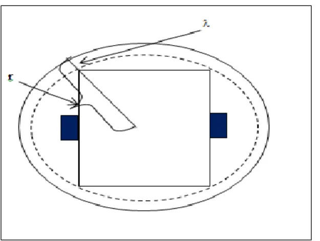
1,O2, . . .,OK}. The whole environment is considered to be in 2D with the objective of simulation. Further we consider a robot which is made up of a series of wheeled robot. The first wheeled robot rake is furnished with range sensor to sense obstacles. Figure 4 illustrates the head of the centipede inspired robot in rectangular shape with wheel and other equipment. The other rakes contain a compact, multi-core propeller microcontroller with hardware to communicate between each. We put the robot and the obstacle in 2D plane and assume a virtual circle surrounding the robot. Every part of the robot will be considered inside a virtual circle. The head and other rakes are same in almost all aspect but the only difference is a sensor is attached with the head which can scan 1800 area. During movement every rake or section of the robot supposed to go after the same coordinates of its predecessor. The initial and final coordinate with respect to global frame of reference is known to robot. Prior we proceed to the description of algorithms, we compose some important and helpful assumption and definition for this algorithm which are almost same as [22].
Figure 2. Centipede like wheeled robot with reference to [23]
Figure 3. Obstacles detected by range
sensor(R) Figure 4. Display of robot and obstacles in 2D plot
2.1.1. Assumption
The robot is supposed be as few physically and analytically connected small robots
The algorithm uses world co-ordinate system as global frame of reference
All position coordinates (including with initial and goal) are at first quadrant
The velocity and angular velocity of robot is constant in every movement and rotation respectively
The environment is flat and maintains equal altitude everywhere
The mobile robot moves in a two-dimensional space and rotates without slipping
Both the robot and dynamic obstacles are run in constant speed and in straight line. If anyone wants to change direction it has to stop then turn then again start moving
2.1.2. Important definitions
The robot scans the surroundings 00 to 1800 by range sensor. So to make a scan of total 3600 the robot has to rotate the head part 900 left and right and scan the environment again. Obviously it is required if the centipede gets full of obstacle at 1800 scan. We consider on bounded and unbounded space O and Q in a reading from range sensor within a time period, tn to tn+1. If it notices a variation in distance say Δd (where Δd value is defined) in range at any position then that position point is regarded as Open Point. The primarily the robot facing directly to goal point and afterward it begins scanning for open point. Sub goal point is a mid objective of the robot to attain the final objective. This point is placed at a particular difference from the corresponding open point and perhaps creates a right angle at open point to the line passing through the sensor point of robot and the open point. From the coordinate of open point corresponding sub goal point is determined. The robot selects one point called critical point, for subsequent move from a set of sub goal points. This point is selected on the base of smallest distance from the target point and so far not considered for movement. The robot attempts to move its each rake’s center of virtual circle to critical point or to virtual circle’s center of its predecessor. The midpoint of the two extreme points of each robot’s rake is centre of the corresponding virtual circle and the half distance between the two extreme points of the rake with a safety constant is the radius. The lowest value of can be obtained from few number of experiments. Figure 4 shows the plotting and other required geometrical details.
d – Perpendicular distance of obstacle from the sensor A – Location of robot wheel-‘axle’ (imaginary line) center X – Distance from sensor to open point
w – Distance between wheel-‘axle’ center and wheel center F – Distance between the rear end and wheel ‘axle’ center
R – Distance between the wheel ‘axle’ center and the rear end of the robot C – Center of the virtual circle
α – Open point detection angle by the sensor
- Safety constant for the robot r – Radious of the virtual circle
β – Sensor direction angle at open point with respect to the line parallel to x-axis and passing through (xi,yi) before movement
θ – Angle generated by β with respect to the line parallel to x-axis for sub goal point coordinates calculation
– Angle created on a line parallel to x axis and passing through sensor by a line from sensor to open point
– Angle between line joining open point & subgoal and the line parallel to x-axis and passing through open point
dk– Distance of a sub goal point from current location
xs and ys – are the sign factors used in determination of the coordinates of open points sx and sy – are the sign factors used to determine the coordinates of sub goal points We consider,
Tn= {(x1,y1),(x2,y2),...,(xi,yi)} as a set points travelled by the robot’s nth link where (xi,yi) symbolize the coordinate values the nth link arrived
OP={((αa,da),(αb,db)),....,((αk,dk),(αj,dj))} as a set of open points of obstacles identified by the sensor where α and d indicate the angles & distances of open points respectively from the robot and each ((αa,da),(αb,db)) represents two open points connected to each obstacle, if only one point is detected then αa=αb and da=db
SG= {(ai,bi),…..,(xj,yj)} as a set of sub goal points recognized by the robot and every (ai,bi) signifies the sub goal point which the robot can select for next move
Tobs= {((ai,bi),…(aj,bj)),…..,((xi,yi),..,(xj,yj))} as a set of initially identified obstruction where each ((ai,bi),…(aj,bj)) are the set of points of each obstacle.
Sobs= {((ai,bi),…(aj,bj)),…..,((xi,yi),..,(xj,yj))} as a set of fixed obstacles where every ((ai,bi),…(aj,bj)) are the set of points of each fixed obstacle.
TDobs= {((ai,bi),…(aj,bj)),…..,((xi,yi),..,(xj,yj))} as a set of initially moving obstacles where every ((ai,bi),…(aj,bj)) are the set of points of each provisionally moving obstacle.
Dobs= {((ai,bi),…(aj,bj)),…..,((xi,yi),..,(xj,yj))} as a set of movable obstacles where each ((ai,bi),…(aj,bj)) are the set of points of each movable obstacle.
D= {((xa,ya),δa),…,((xj,yj),δj)} as a set of sub goal points and distance from target of that point where each set ((xa,ya),δa) represents the set of sub goal point and their distance from target
Here dmin is the distance from the robot to goal point and is the direction of the same.
PC is the position where the robot may collide with the obstacle and the distance from current position of robot to the point of collision is DC.
Development of path planning algorithm of centipede inspired wheeled robot... (Subir Kumar Das) 2.1.3. Algorithm
a. Main procedure 1. Robot Start
2. Take input of the position co-ordinates of source and destination
3. Calculate the distance and direction from source to destination dmin and respectively 4. WHILE not Destination
5. Start OBSTACLE_DETECTION procedure in FOV 6. IF obstacle or virtual obstacle in direction
7. Calculate the coordinates of sub goals from OP, don’t calculate same set from OP twice and save it in set SG and D
8. Calculate distance of each sub goal from destination and save it in set D 9. Select the coordinate point P having the lowest distance in D
10. IF the point exists in Traverse point set T1
11. Discard the point
12. Select the next lowest distance point P from D
13. Follow step 10
14. ELSE
15. IF P is SAFE_POINT
16. Save the coordinate in traverse point set T1 17. Calculate angle of rotation and rotate
18. Call MOVE Procedure to move at P
19. IF obstacle dynamic
20. IF VIRTUALOBSTACLE
21. Follow step 7
22. END IF
23. END IF
24. Calculate direction and distance dmin
25. ENDIF
26. ENDIF
27. ELSE
28. Calculate the next point coordinate P towards the direction
29. IF P is SAFE_POINT
30. Save the coordinate in T1
31. Call MOVE Procedure to move at P
32. Calculate new dmin
33. END IF
34. END IF
35. END WHILE 36. Robot Stop b. Move procedure 1. FOR i=n to 2
2. Save the last coordinate of Ti-1 in traverse point set Ti 3. END FOR
4. FOR i=1 to n
5. Move the ith link toward the last point of Ti 6. END FOR
c. Obstacle_detection procedure 1. Scan 00 to 1800
2. Identify obstacles in FOV
3. Calculate the coordinates of open points and save those points in set Tobs 4. IF no open points
5. Rotate the head left 900 6. Scan 00 to 1800
7. Calculate the coordinates of open points and save those points in set Tobs 8. Rotate the head right 900
9. Scan 00 to 1800
10. Calculate the coordinates of open points and save those points in set Tobs 11.END IF
13. IF coordinate set of Tobs exists in Sobs 14. Discard the coordinate from Tobs
15. ELSE
16. IF there exists any nearest point in Sobs with small change in x or y value 17. The obstacle may be dynamic
18. Save coordinate in TDobs
19. ELSE
20. IF there exists any nearest point in TDobs with small change in x or y value 21. It is part of moving obstacle
22. Save the points of TDobs and Tobs to the robot registry and all the open points of the obstacle in Dobs
23. ELSE
24. Save the points in Sobs
25. RETURN obstacle
26. END IF
27. END IF
28. END IF
29.END FOR
30.IF obstacle dynamic
31. IF VIRTUALOBSTCLE
32. RETURN virtual obstacle
33. END IF
34.END IF
d. Virtualobstacle procedure
1. Calculate direction and speed vobs of the obstacle from the points exists in robot registry 2. IF the obstacle direction intersecting robot direction
3. Calculate probable position PC of collision
4. Calculate probable distance DC from the robot to PC 5. IF DC<dmin
6. Calculate the time RTC1 and RTC2 the robot will take to arrive at PC and cross PC fully respectively
7. Calculate the time OTC moving obstacle will requires to arrive at PC 8. IF RTC2>=OTC and RTC1<=OTC
9. Identify the point PC and all the adjacent points of the obstacle as virtual Obstacle 10. Calculate the open points and save in OP
11. RETURN virtual obstacle
12. ENDIF
13. END IF
14.END IF
e. Safe_point procedure
1. IF P corresponds to a sub sub set of OP
2. Select the sub set from OP that corresponds to P 3. IF it is first sub set
4. Select the second sub set from previous set from OP
5. ELSE
6. Select the first sub set from next set from OP
7. END IF
8. Calculate the distance Sd between two sub sets 9. ELSE
10. Select the two points from OP having minimum distance from P 11. Calculate the distance Sd between two points
12. END IF 13. IF Sd < 2r
14. RETURN safe 15. ELSE
16. RETURN not safe 17. ENDIF
Development of path planning algorithm of centipede inspired wheeled robot... (Subir Kumar Das) 3. DISCUSSION AND RESULT
The principle motive of the algorithm is to create a continuous path from fixed source to destination. Avoiding static obstacle can be is discussed in [20-21], the Figure 1 shows the avoidance as per [20]. Current algorithm attempts to avoid moving obstacle too. Also this algorithm in contrast of [21], judges the robot as a series of rakes having dimensions not only a point and averts collision with the obstacles using preventative measure. Figure 5 shows each part of the robot considering in a virtual circle avoid obstacle and the open points and its related sub goal points is shown in Figure 6 Calculating sob goal point using required methodology is reflected in Figure 7 All the sub goals situate perpendicularly reverse direction of the related open points. To avoid the obstacle the robot has to turn the rakes. The turning angle and displacement of robot’s position due to turn is shown in Figure 8.
Figure 5. Whole robot inside the virtual circle with safety measurement
Figure 6. Obstacles’ open point and sub goal point detected by robot
3.1. Algorithm study and analysis
Let an open point is identified by sensor at angle α. As per [20]
βi= (α +βi-1)%360
xi+1,j = x+dkcosθ(xs) (1)
yi+1,j = y+dksinθ(ys) (2)
Here (x,y) is the location of sensor and (xi+1,j,yi+1,j) is the location of jth identified, one of subsequent open points at (i+1)th iteration and in accordance to worlds coordinate system. The open point appears in two ways. 1. If earlier value of α, the sensor angle α -1 senses an obstruction and 2. Subsequent value of α, the sensor angle α+1 senses obstruction. Each of these two also have two sub cases and those are: a) > 900 and b) <= 900
where =%180° So we can describe as follows,
= {
− 90°, Sx = 1, Sy = 1 if > 90° − 1 not obstacle
− 90°, Sx = −1, Sy = −1 if > 90° − 1 is obstacle
90° −, Sx = 1, Sy = −1 if ≤ 90° − 1 not obstacle
90° −, Sx = −1, Sy = 1 if ≤ 90°− 1 is obstacle
(3)
If (xi+1,j,yi+1,j) is open point P then as per Figure 7, coordinate value of connected sub goal point Q is:
𝑄𝑥 = 𝑃𝑥 + 𝑆𝑥. 𝑟𝑐𝑜𝑠
𝑄𝑦 = 𝑃𝑦 + 𝑆𝑦. 𝑟𝑐𝑜𝑠} (4)
(Qx,Qy) will be the next centre after move of the virtual circle that contains the head part of centipede inspired robot. In accordance to Figure 4, A is the wheel axel centre and AC is the distance among the virtual circle centre and wheel axel centre. So, the value of next position of wheel axel centre A can be determined as,
𝐴𝑥 = 𝑄𝑥 + 𝑆𝑥. 𝐴𝐶𝑐𝑜𝑠
𝐴𝑦 = 𝑄𝑦 + 𝑆𝑦. 𝐴𝐶𝑠𝑖𝑛 } (5)
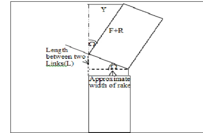
Now the head part of robot will compute the required angle of rotate to move wheel axel centre and then start progressing to next position. The remaining part of the robot will follow it predecessor links coordinate location for next move as written in algorithm. During its turning to avoid obstacles the robot gets displaced from its dmin line, which it has to cover in near future. Maximum it turns the maximum it takes to cover. According Figure 8, if Y is the displacement value then,
Y = (F + R)sin (6)
= sin−1𝑌 (𝐹 + 𝑅)⁄ (7)
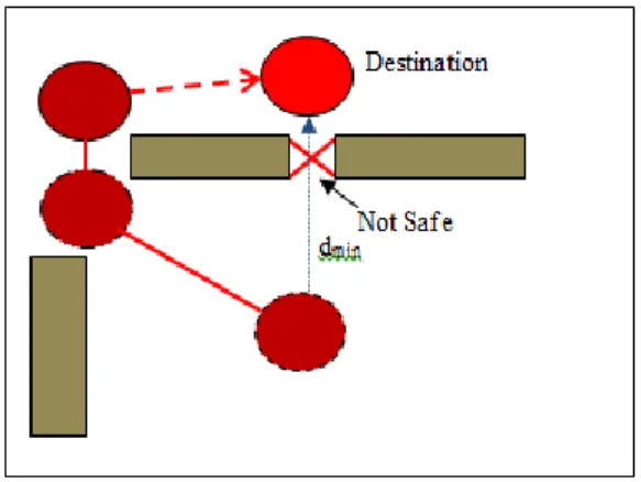
Here (F+R) is the length of each rake and is the maximum permissible rotation angle of a rake. Irrespective of mobility or non-mobility every obstacle is stationary at an exact point of time. If the position changes of an obstacle then it is moving otherwise it is static. For moving obstacle the possible position in future can be determined from its speed and direction. Figure 9 illustrates how to avoid dynamic obstacle using MCSB algorithm by predicting the virtual obstacle location. The stated scheme allows the robot to avoid securely static obstacles shown in Figure 10. For mobile obstacles is has find out the speed of that obstacle by sensing its position at two separate time tn+1 and tn where t=tn+1-tn. Therefore,
Figure 7. Open point to Sub goal point calculation Figure 8. Turning angle and displacement during turn
Figure 9. Avoiding a moving obstacle by calculating virtual obstacle twice
Development of path planning algorithm of centipede inspired wheeled robot... (Subir Kumar Das)
vobs=(Ot+1−Ot t) (9)
where Ot+1,Ot are Obstacle positions at time instant tn+1 and tn and vobs is speed of the mobile obstacle. By solving equation of robot’s direction and obstacle’s direction the probable position of collision (PC) can be calculated. The next task is to find out whether there will be a real collision or not at PC. If there will be a collision then the position and its surrounding will be identified as virtual circle. If PR(rxn+1,ryn+1)be current location of the robot at tn+1. Then,
DC= √(Cx − rxn+1)2+ (Cy − ryn+1)2 (10)
where (Cx,Cy) is the coordinate position of PC. By the value of DC robot then determines,
RTC1= DC⁄ v (11)
RTC2= (n ∗ 2r + DC)⁄ v (12)
OTC= DC⁄vobs (13)
The velocity of robot is v. RTC1 and RTC2 are time of entering at PC and exiting from PC respectively and OTC is the time the obstacle will take to arrive at collision point. N is number of links or rakes of the robot and r is the radius of virtual circle. OTC lies time range RTC1 and RTC2 means they will be at PC in the same time period in near future. So the point will be indicated as virtual obstacle and distorted trajectory will be shaped with safety measure. How the robot will avoid local minima problem is illustrated in Figure 9. If the robot fails to find an open point in direction FOV the head will rotate right and left as much as possible, scan the area take open points. If it still fails then it has to rotate the whole robot. The Figure 11 shows how to avoid an obstacle with safety measurement. Here in this figure it is described for a single link. But for any links it is applicable as all the links follow the same path to reach destination.
Figure 11. Obstacle avoidance with safety measurement
3.2. Total time and path length calculation
If vi and i are the speed and angular velocity at ith iteration then, time taken in moving and rotating [20]:
𝑇𝑀= ∑𝑛𝑖=0𝑑𝑖⁄𝑣𝑖
𝑇𝑅= ∑𝑛𝑖=0𝑖⁄𝑖
So the cost function in terms of time for one links is:
𝐶 = ∑(𝑑𝑖⁄ + 𝛼𝑣𝑖 𝑖⁄ )𝜔𝑖
𝑛
𝑖=0
+ ∑ 𝐷𝑂𝑇
𝑚
where DOT is the time taken to identify mobile obstacle and its direction of progress and speed. So the total cost in terms of time for all the links or the whole robot is:
𝑇𝐶 = ∑ 𝐶𝑖
𝑛
1
3.3. Simulation results
How a robot is using ModifiedCritical-Snakebug algorithm to stay away from stationary and non-stationary obstacle shown in the Figure 12. There are twelve separate snap shots of twelve separate moments in same environment. The gray coloured, rectangular shaped object is non-stationary obstacle and static obstacles are of green rectangular. The algorithm is modelled using Python 3.5 on windows 7 platform. Intel core [email protected] Ghz Laptop with 2 GB RAM is used. The red circle at the top and foot are the goal and initial points respectively. The path robot travelled is shown using Black line.
Figure 12. Snapshots of trajectory generated using modifiedcritical-snakebug algorithm on 2D plane
4. CONCLUSIONS AND FUTURE WORK
The earlier works is further continued in this paper. The foremost intention is to build a local path planning algorithm on simple sensor based for bio-inspired centipede like multi rake robot. The algorithm makes an effort to think about the restrictions of robot’s dimension. To complete the task using this bug algorithm the robot requires very little prior information. Measuring the safety precaution makes the algorithm more effective. This algorithm helps to avoid a very small the gap or to pass through small gap which is big enough to pass. In case less complex environment or environment with few numbers of obstacle,
Development of path planning algorithm of centipede inspired wheeled robot... (Subir Kumar Das) the algorithm and other algorithm doing the same task may take approximately same time. Few favorable points of this algorithm are: (a) It never judges the all the obstacles for avoidance. (b) Uses well-organized technique to estimate coordinates of different points. (c) It is an algorithm for multi rake robot to avoid any obstacles of regular shape. (d) Tries to take as possible as less time to reach at destination. The algorithm will be used to test real multi rake robot in the future,. Further it will be studied using camera vision for snake like robot and for multiple robots path planning in one environment.
ACKNOWLEDGEMENT
Thank you to Production Engineering Department, Jadavpur University and Asansol Engineering College for giving us the opportunity to use their resources.
REFERENCES
[1] Farah Kamil, Tang Sai Hong, Weria Khaksar, Mohammed Yasser Moghrabiah, Norzima Zulkifli, Siti Azfanizam Ahmad, “New robot navigation algorithm for arbitrary unknown dynamic environments based on future prediction and priority behaviour”, Expert Systems With Applications, 86, 2017, 86, 274 – 291
[2] David L. Hu, Jasmine Nirody, Terri Scott, Michael J. Shelley, The mechanics of slithering locomotion, PNAS, 2009; 106(25), 10081–10085
[3] Kristin Y. Pettersen, “Snake Robots”, Annual Reviews in Control, 2017; 44, 19–44
[4] Zhenli Lu, Dayu Feng, Yafei Xie, Huigang Xu,Limin Mao, Changkao Shan, Bin Li, Petr Bilik, Jan Zidek,Radek Martinek, Zdenek Rykala, “Study on the motion control of snake-likerobots on land and in water”, Perspectives in Science, 2016; 7, 101—108
[5] Bernhard Klaassen, Karl L. Paap, “GMD-SNAKE2 a snake-like robot driven by wheels and a Method for Motion Control”, Proceedings of 1999 IEEE International Conference on Robotics and Automation
[6] Tetsushi Kamegawa, Toshimichi Baba, Akio Gofuku, “V-shift control for snake robot moving the inside of a pipe with helical rolling motion”, Proceedings of the 2011 IEEE International Symposium on Safety,Security and
Rescue Robotics, 2011;1-6
[7] Gabriel Ford, Richard Primerano, Moshe Kam, “Crawling and rolling gaits for a coupled mobility Snake Robot”,
The 15th IEEE International Conference on Advanced Robotics, 2011;556-562
[8] Katie L. Hoffman, Robert J. Wood, “Turning gaits and optimal undulatory gaits for a modular centipede-inspired millirobot”, The Fourth IEEE RAS/EMBS International Conference on Biomedical Robotics and Biomechatronics,
2012; 1052-1059
[9] L. Pfotzer, S. Klemm, A. Roennau, J.M. Zöllner, R. Dillmann, “Autonomous navigation for reconfigurable snake-like robots in challenging, unknown environments”, Robotics and Autonomous Systems, 2017; 89, 123–135 [10] Filippo Sanfilippo, Jon Azpiazu, Giancarlo Marafioti, Aksel A. Transeth, Øyvind Stavdahl, Pål Liljebäck,
“Perception-Driven Obstacle-Aided Locomotion for Snake Robots-The State of the Art, Challenges and Possibilities”, Applied Science, 2017; 7, 336, 1-22
[11] Sahin Yıldırım, Ebubekir Yasar, “Development of an obstacle-avoidance algorithm for snake-like robots”,
Measurement, 2015; 73, 68 – 73
[12] Y. Cheng, P. Jiang, Y. F. Hu, “Snakebased scheme for path planning and control with constraints by distributed visual sensors”, Robotica, 2014; 32, 477–499
[13] Jin Cheng, Yong Zhang, Zhonghua Wang, “Motion Planning Algorithm for Tractor-trailer Mobile Robot in Unknown Environment”, 8th International Conference on Natural Computation (ICNC 2012), 2012; 1050 – 1055 [14] Akash Singh, Anshul, Chaohui Gong, Howie Choset, “Modelling and Path Planning of Snake Robot in cluttered
environment”, CoRR, 2017; abs/1710.02610, 1 – 7
[15] Y. Cheng, P. Jiang, Y. Fun. Hu, “A Distributed Snake Algorithm for Mobile Robots Path Planning with Curvature Constraints”, IEEE International Conference on Systems, Man and Cybernetics (SMC 2008), 2008; 2056 – 2062
[16] Ehsan Rezapour, Kristin Y Pettersen, Pål Liljebäck, Jan T Gravdahl, Eleni Kelasidi, “Path following control of planar snake robots using virtual holonomic constraints-theory and experiments”, Robotics and Biomimetics, 2014; 1(3), 1- 15
[17] Jinguo Liu, Yuechao Wang, Bin Ii, S. Ma, “Path Planning of A Snake-Like Robot Based on Serpenoid Curve and Genetic Algorithms”, Fifth World Congress on Intelligent Control and Automation (IEEE Cat. No.04EX788), 2004;
4860 – 4864
[18] Spenneberg Dirk, Kirchner Frank, “The Bio-Inspired SCORPION Robot Design,Control & Lessons Learned”,
Climbing & Walking Robots, Towards New Applications, ISBN 978-3-902613-16-5, 2007; 197 – 218
[19] Bernhard Klaassen, Ralf Linnemann, Dirk Spenneberg, Frank Kirchner, “Biomimetic walking robot SCORPION Control and modeling”, Robotics and autonomous systems, 2002; 41(2-3), 69 – 76
[20] Keith Kotay, Daniela Rus, “The Inchworm Robot: A Multi-Functional System”, Autonomous Robots, 2000; 8, 53– 69
[21] Ajoy Kumar Dutta, Subir Kumar Debnath, Subir Kumar Das, “Local Path Planning of Mobile Robot Using Critical-PointBug Algorithm Avoiding Static Obstacles”, IAES International Journal of Robotics and Automation (IJRA), 2016; 5(3), 182 – 189
[22] Ajoy Kumar Dutta, Subir Kumar Debnath, Subir Kumar Das, “Path-Planning of Snake-Like Robot in Presence of Static Obstacles Using Critical-SnakeBug Algorithm”, Advances in Computer, Communication and Control, 449-458
[23] https://tamiyablog.com/2018/06/customizing-the-tamiya-70230-centipede-robot-to-18-wheel-drive-car/
BIOGRAPHIES OF AUTHORS
Dr. Ajoy Kumar Dutta is currently a Professor in the Department of Production Engineering, Jadavpur University, INDIA. He received his B. E. & M. E. degrees in Electronics & Tele-communication Engg from Jadavpur University in 1983 & 1985 respectively, and Ph. D. (Engg) degree in the area of Robotics from Jadavpur University in 1991. His Field of Specialization and Research Area are Robotics, Sensors, Computer Vision, Microprocessor Applications, and Mechatronics. He has teaching & research experience of 31 years.
Mr. Subir Kumar Debnath is currently an Associate Professor in the Department of Production Engineering, Jadavpur University, INDIA. He received his B. E. degree in Mechanical Engg from Jadavpur University in 1982 & M. Tech in Mechanical Engg in 1984 from I.I.T.- Kharagpur, INDIA. His Field of Specialization and Research Area are Robotics, Sensors, Computer Vision, CNC Machines and Automation. He has teaching & research experience of 31 years.
Subir Kumar Das received M.Tech Operations Research in 2010 and M.Sc. Computer Science in 2007. He is currently pursuing a Ph.D. from Jadavpur University of India. His research interests include computer vision system, autonomous mobile robots, optimisation technique.
![Figure 1. Trajectories formed by different bug algorithm with reference to literature [20]](https://thumb-us.123doks.com/thumbv2/123dok_us/8384724.2227772/2.893.347.570.794.1073/figure-trajectories-formed-different-bug-algorithm-reference-literature.webp)
![Figure 2. Centipede like wheeled robot with reference to [23]](https://thumb-us.123doks.com/thumbv2/123dok_us/8384724.2227772/3.893.127.790.703.929/figure-centipede-like-wheeled-robot-reference.webp)