www.elsevier.com / locate / ijforecast
A
genetic algorithms approach to growth phase forecasting of
wireless subscribers
1
*
,2Rajkumar Venkatesan , V. Kumar
ING Center for Financial Services, School of Business, University of Connecticut, Storrs, CT 06269-1041, USA
Abstract
In order to effectively make forecasts in the telecommunications sector during the growth phase of a new product life cycle, we evaluate performance of an evolutionary technique: genetic algorithms (GAs), used in conjunction with a diffusion model of adoption such as the Bass model. During the growth phase, managers want to predict (1) future sales per period, (2) the magnitude of sales during peak, and (3) when the industry would reach maturity. At present, reliable estimation of parameters of diffusion models is possible, when sales data includes the peak sales also. Cellular phone adoption data from seven Western European Countries is used in this study to illustrate the benefits of using the new technique. The parameter
¨
estimates obtained from GAs exhibit good consistency comparable to NLS, OLS, and a naıve time series model when the entire sales history is considered. When censored datasets (data points available until the inflection point) are used, the proposed technique provides better predictions of future sales; peak sales time period, and peak sales magnitude as compared to currently available estimation techniques.
2002 International Institute of Forecasters. Published by Elsevier Science B.V. All rights reserved.
Keywords: New product diffusion-estimation; Genetic algorithms; Telecommunication industry; Bass model
Forecast). Specifically the sales of mobile
wire-1
. Introduction
less phones worldwide increased by 46% in The telecommunication industry has ex- year 2000. Also, by the end of 2001, European perienced rapid growth in the recent years and Mobile Communications (EMC) forecasts world is forecasted to exceed $790B in revenues by cellular subscriptions to top the one billion 2003 (2000 Multimedia Telecommunications mark, up from 728 million at year end 2000. The sustained tremendous growth in the wire-less communications industry over the past *Corresponding author. Tel.: 11-860-486-1086; fax:
11-860-486-8396. decade also aggravates the need for accurate E-mail addresses: [email protected] (R. forecasts of future growth potential. The Venkatesan),[email protected] (V. Kumar). ubiquitous product life cycle would suggest that 1
Rajkumar Venkatesan is an Assistant Professor in
Market-a phMarket-ase of consolidMarket-ation Market-and decline in growth
ing.
2 is imminent. In that case, when is it supposed to
V. Kumar (VK) is the ING Chair Professor and Executive
happen?
Director.
0169-2070 / 02 / $ – see front matter 2002 International Institute of Forecasters. Published by Elsevier Science B.V. All rights reserved. P I I : S 0 1 6 9 - 2 0 7 0 ( 0 2 ) 0 0 0 7 0 - 5
Sales forecasts during the early stages of a just the time since a product has been intro-product life cycle are critical to both new duced in the market for making reliable fore-product managers and academicians. The casts of the future sales of the innovation. In growth phase of the product life cycle is char- addition to providing reliable forecasts, the Bass acterized by high growth in sales and market model has attractive behavioral implications expansion. Also, the marketing strategy in the regarding customer motivation that could assist growth phase is characterized by heavy adver- managerial decision-making.
tising as compared to heavy promotions in the Since its introduction, the Bass (1969) model maturity / decline stage (Kotler, 2000). Given of innovation adoption has spawned a wide the implications to marketing strategy, predict- range of applications and models that explain ing the future sales during the growth phase is the rate of adoption of an innovation (Bayus, of paramount importance. In addition to predict- 1992), the effect of marketing mix variables on ing the future sales of the product, managers the market potential and rate of adoption of an need to know when the product would reach innovation (Bass, Krishnan, & Jain, 1994; Jain maturity and what the value of sales would be at & Rao, 1990; Kalish, 1983; Bass, 1980; Robin-maturity. Accurate knowledge about the time to son & Lakhani, 1975), and diffusion of innova-peak sales helps managers deduce the growth tions in multiple markets (Krishnan, Bass, & rate of their markets, and the marketing mix Kumar, 2000; Kumar, Ganesh, & Echambadi, necessary to accelerate the sales of their new 1998; Takada & Jain, 1991). Even the basic innovation. Appropriate forecasts of future Bass diffusion model has been modified to growth potential are essential for proper man- accommodate for time-varying parameters, flex-agement of resources, and further have im- ibility in the shape of the diffusion pattern, and portant profit implications. evaluating marketing strategies that are effective Several micro-level telecommunications de- in various stages of the product life cycle, and mand models have been proposed (Fildes, influence of another country on one country’s 2002) that accommodate characteristics such as diffusion (Kumar & Krishnan, 2002; Ganesh, network effects, price elasticity, government Kumar & Subramaniam, 1997). Forecasting of regulations, incentive structures and product future sales, a critical application of the Bass quality. The micro-level models seem to work diffusion model, has received little or no atten-well in established markets and for new prod- tion because researchers are faced with difficul-ucts / services the reliance is more on qualitative ties in using the Bass model for this purpose measures such as expert / consumer opinion. In (Parker, 1994). The forecasting of future sales addition to micro-level models, managers are of a new product before the inflection point in also interested in forecasting the macro-level the product life cycle is reached is a particularly growth for a new market over a fixed time critical drawback (Mahajan, Muller, & Bass, horizon in order to assist decision-making and 1990).
strategy development. The macro-level models Ordinary Least Squares (OLS), Maximum that are used need to be parsimonious and are Likelihood, and Non-linear Least Squares mostly used in combination with micro-level (NLS) procedures have been proposed in the models for decision-making. Several macro- literature for estimating the parameters in a Bass level time series models including logistic diffusion model. However each technique has growth curves have been proposed to predict the its own shortcomings with respect to providing future category level sales of an innovation. The reliable and accurate forecasts of product sales / Bass (1969) model is one such model that uses growth. The estimates based on OLS are biased
because OLS (1) assumes a discrete process for unreliable. In the continuous time framework, data generated from a continuous process, (2) the reliable estimation of the Bass model is suffers from multicollinearity, and (3) does not possible only when the inflection point in the generate standard errors directly for p, q, and m product life cycle is available for estimation. which makes testing hypotheses impossible. The Hence, the utility of the Bass model is con-estimates based on maximum likelihood are strained by lack of appropriate estimation tech-efficient in reducing sampling errors associated niques and is currently used primarily for with survey based data but are not efficient in retrospective analysis. By the time sufficient reducing errors related to measuring exogenous observations have been collected for reliable factors such as marketing mix. The NLS esti- estimation, it is too late to use the estimates for mates suffer from ill-conditioning (Van den forecasting purposes (Mahajan et al., 1990). Bulte & Lilien, 1997), which makes the esti- Current forecasting techniques, based on the mates proportional to the number of data points Bass model, in general require educated guesses available for estimation. Van den Bulte and from managers about either (1) the eventual Lilien (1997) and Srinivasan and Mason (1986) market potential of a product (m), (2) time of show that the estimates of the Bass model the peak of the non-cumulative adoption curve, (derived from Non-linear Least Squares) are and (3) the sales at the peak time period biased (or in most cases do not converge) when (Mahajan & Sharma, 1986), or (1) the eventual used for making predictions regarding future market potential of a product (m), (2) the sales sales during the growth phase of the product life during the first time period, and (3) an estimate cycle. Also, the estimates obtained are corre- of the sum of the coefficient of innovation ( p), lated to the number of data points used for and the coefficient of imitation ( q) (Lawrence & estimation. Specifically, the estimate of market Lawton, 1981). The initial guesses are based on potential, m, is downward biased when fewer data from industry reports, surveys, test-market-data points are used for estimation and vice- ing sales and from diffusion estimates of ana-versa for the coefficient of imitation q. This bias logical products. In a review of models avail-and systematic change in parameter estimates is able for forecasting diffusion of innovations, attributed to ill-conditioning—a problem that Meade and Islam (2001) conclude that current exists in intrinsically non-linear models that are evidence suggests that judgmental estimates of estimated using Non-linear Least Squares market potential contribute little to the accuracy (NLS) (Seber & Wild, 1993; Van den Bulte & of forecasts of future sales. The econometric Lilien, 1997; Venkatesan, Krishnan, & Kumar, procedures used for estimating the Bass model 2001). These issues associated with the widely such as Ordinary Least Squares (OLS) (Bass, adopted NLS technique for estimation of the 1969), Maximum Likelihood estimation Bass model have left forecasters with few (Schmittlein & Mahajan, 1982), and Non-linear ‘rules-of-thumb’ or empirical generalizations to Least Squares (NLS) (Srinivasan & Mason,
work with. 1986) have individual drawbacks and are all not
In the discrete version of the Bass model useful for generating forecasts during the (OLS estimation) and in a majority of the cases, growth phase of the diffusion curve. Hierarchi-there is no restriction on the number of data cal Bayes procedures to predict the sales of new points required for estimation. However, with products before peak sales are weak when the OLS the estimates of the Bass model cannot be new product takes time to take off, or in other bounded and in a majority of the cases the words is left skewed (Lenk & Rao, 1990). estimates obtained with fewer data points are In this study, we evaluate the performance of
a simple simulation based search technique— (1986) operationalization, which can be repre-Genetic Algorithms (GAs)—for forecasting the sented as
magnitude of future sales, time period to peak X(t)5m[F(t)2F(t21)]1e (1) sales, and the value of sales during peak time
2( p1q)t 2( p1q)t
period using the Bass model when only a few F(t)5(12e ) /(11( q /p)e ) (2) data points are available, i.e., well before the
where X(t)5sales at time t, m5number of inflection point for the new product is reached.
eventual adopters, F(t)5cumulative distribution GAs are parallel search algorithms that are
of adoptions at time t, p5coefficient of innova-based on an analogy with Darwin’s theory of
tion, and q5coefficient of imitation. e5
evolution to converge to a global minimum in a
normally distributed random error term with given search space. The inherent nature of GAs
2
mean zero and variance s . ensures that the estimates are robust even with a
The density function ( f(t)) or each period small number of data points irrespective of the
sales is obtained by differentiating (2) with functional form of the objective function. These
respect to t, (i.e.), features of GAs make them an excellent
candi-date for forecasting purposes, with non-linear 2 2( p1q)t 2( p1q)t 2
f(t)5(( p1q) /p)*e ) /(11( q /p)e ) models such as the Bass model. In order to
(3) establish the reliability and validity of estimates
generated from GA, and to evaluate the utility Finally, the time to peak period sales (T *) is of the estimates for hypotheses testing, the obtained by differentiating (3) and solving for t, performance of GAs is compared with tech- which yields
niques such as NLS and OLS and the finite
T *5[1 /( p1q)]*ln( q /p) (4)
sample properties of the estimates from GAs are
also derived. The level of sales at peak is given by
substitut-In the next section we provide an overview of ing 4 in 3, i.e., past research in forecasting sales using Bass
2
X(T *)5m*[(1 /(4q))*( p1q) ] (5) models, in Section 3 we provide a simple
description of genetic algorithms, Section 4
The inflection point for each period sales is explains the design and results of the study obtained by differentiating (3) twice, with re-which compares the performance of GAs, NLS
spect to t, and solving for t, which yields, and OLS in forecasting the time to peak sales
1 q
for cellular phones in seven different countries Œ]
]] ]
s
d
Tleft**5 *ln
S D
* 22 3 (6a)p1q p
in Western Europe, finally the conclusions,
limitations, and future research directions are 1 q
]
Œ
]] ]
s
d
T **5 *ln * 21 3 (6b)
provided in Section 5. right p1q
S D
pIt is useful to note here that the time for peak period sales depends only on the hazard rate
2
. Conceptual background
parameters p and q, and is independent of the
3 market potential m. This is also intuitive if we
2
.1. Model formulation
believe that the hazard rate determines the shape We choose to use the Srinivasan and Mason of the diffusion curve and hence also determines the time of peak sales. The market potential
3 term, m, provides only the level effect to the
Please refer to Fildes (2002) for a discussion of various
sales at T *. In order to obtain reliable estimates with the new information to form posterior of p, q, and m before the peak sales is reached estimates of the new product sales. The updat-data is required until Tleft**; which represents ing procedure resembles a weighted sum of the the take-off period for any new product. initial estimates from similar products and esti-mates derived from the new sales data. During the early stages of the product life cycle, the
2
.2. Forecasting with commonly employed
initial estimates from sales of similar products
estimation techniques
carry more weight but as more new information is obtained, i.e., later in the product life cycle, The shortcomings associated with the current
the estimates based on sales of the new product estimation techniques (as explained earlier) have
carry more weight. The strength of the Hierar-led researchers to adopt subjective techniques
chical Bayes procedure lies in accommodating for forecasting adoption of new product
accept-the heterogeneity between and within product ance as described below. Current procedures to
sales curves when obtaining initial estimates. forecast future sales, time to peak period, sales
However, estimates from these procedures are at the peak period of new products hence
not accurate when the new product diffusion involve variations of the following steps
(Law-curve is skewed away from the near symmetric rence & Lawton, 1981; Mahajan & Sharma,
Bass model assumption. 1986; Modis & Debecker, 1992):
Subjectivity involved in the above procedures has led researchers to conclude that ‘‘parameter • Managers make an educated guess about the
estimation for diffusion models is primarily of parameters a (coefficient of external
influ-historical interest; by the time sufficient ob-ence: p), b (coefficient of internal influob-ence:
servations have been developed for reliable
q) and m (market potential).
estimation, it is too late to use the estimates for • These are then used to derive the diffusion
forecasting purposes’’ (Mahajan et al., 1990). curve algebraically.
Hyman (1988) also concluded similarly that • Once the first year sales data (N(1)) becomes
waiting for enough observations to fit the cor-available, the value of a can be updated as:
rect model renders the benefits of the
forecast-a5N(1) /m
ing exercise a moot issue. • The diffusion curve is derived again using
Considering the significant advantages of the updated parameters.
accurate forecasts of product life cycle stages, • As more data becomes available the forecasts
we propose a scientific method,Genetic Algo-are revised or updated based on techniques
rithms, to estimate the diffusion model and such as the adaptive Bayesian feedback filter.
forecast the diffusion curve of a new product The estimate for market potential can be once a minimum number of data points be-obtained from pre-launch purchase intention comes available (about 4–5 data points). Given measures (Jamieson & Bass, 1989). The esti- the subjectivity involved in current techniques mates for p and q, however, need to be based on this is a significant contribution to both the management judgment or based on estimates literature and the practitioners. Even a small from analogical products. Lenk and Rao (1990) increase in the accuracy of prediction can result suggest a Hierarchical Bayes procedure to ob- in a significant increase in profits for the tain initial estimates (priors) of p and q, based organization. This fact is even more critical on product sales for similar new product adop- given that even a small change in the parame-tion curves. As sales data for the new product is ters p and q can generate significantly different obtained the initial prior estimates are updated diffusion curves. In the next section, we discuss
the theoretical background of genetic algorithms solution vector inherits traits from both its and their application to the modeling and fore- parent solution vectors. Thus, as iterations con-casting of Bass diffusion models. tinue from one generation to the next, traits most favorable to reaching a solution thrive and grow, but those least favorable die out. Eventu-ally, the initial population evolves to one that
3
. Genetic algorithms
contains a solution to the optimization problem As posited by Goldberg (1989), Genetic and the iterations terminate.
Algorithms are search algorithms based on the The genetic algorithm has two main limita-mechanisms of natural selection and natural tions. First, a genetic-algorithm search can genetics. In other words, the genetic algorithm entail many evaluations of the objective func-iterates toward a global solution through a tion and, consequently, much execution time. process that in many ways is analogous to the This is a significant problem with large datasets. Darwinian process of natural selection. However, the Bass (1969) model uses annual Given a specified optimization problem, the sales data and a typical sample size is around algorithm starts with the initial set (population 15–20. Also, given the present rate of progress hereafter) of random candidate solution vectors in computer technology the required computa-(the first generation) and then selects a subset of tional expense is most likely a temporary limita-the population to contribute offsprings to limita-the tion. The second limitation is that, like other next generation of candidate solution vectors. direct search methods, convergence of the ge-The key to this process is selectivity. Not all netic algorithm does not necessarily occur at a population members are given an equal chance single optimum solution. The search will typi-of contributing typi-offspring to the next generation cally find a point that is close enough to the so that only a select few actually contribute. In maximum. A gradient-type algorithm can then particular, population members most likely to be used along with the genetic algorithm so as contribute are those possessing traits favorable to efficiently converge to the maximum. The to solving the optimization problem; least likely genetic algorithm is best viewed as a potentially to contribute are those possessing unfavorable valuable complement rather than a substitute for traits. For example, if the solution vector con- traditional algorithms. The complexity of coding sists of parameter estimates for a diffusion involved in implementing genetic algorithms is model, solution vectors that minimize the sum a major impediment to its widespread ap-of squares ap-of errors (SSEs) are more likely to be plicability. However, many software packages selected than others. In this way, a new popula- (GA toolboxes for use with MatLab, S-Plus, tion of candidate solutions (the second gene- C1 1, and Excel) are being released with wide-ration) is built from the most desirable traits of ranging functions and applications of genetic the initial population. The power of genetic algorithms built into them that can be run even algorithms rests on the operations that are in commonly used spreadsheets.
performed on the new population. Just as in
natural systems where the children inherit traits 3 .1. How the algorithm works
from both their parents, in genetic algorithms a
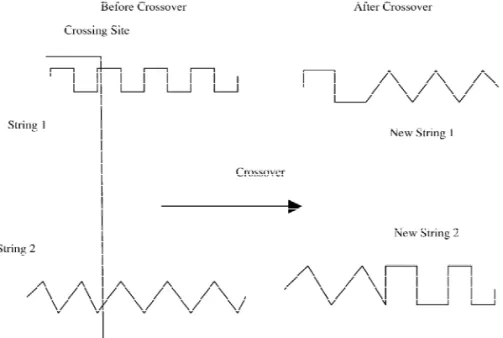
candidate solution vector in the new generation The mechanics of a simple genetic algorithm has two parent solution vectors selected from are surprisingly simple, involving nothing more the previous generation and operations such as complex than copying solution vectors (strings) crossover and mutation (explained later) per- and swapping partial solution vectors (strings). formed on the offspring ensure that the new Simplicity of operation and power of effect are
two of the main attractions of the genetic strings undergoes crossing over as follows:
algorithm. an integer position K along the string is
A simple genetic algorithm that yields good selected uniformly at random between 1 and results in many practical problems is composed the string length less one [1, l21]. Two new of three operators: reproduction, crossover, and strings are created by swapping all characters mutation. A genetic algorithm iterates through between positions K11 and l. This process
4
the following three steps (Fig. 1 illustrates the is explained in Fig. 2 . The mechanics of cycle of steps in a Genetic Algorithm): reproduction and crossover are surprisingly simple, involving random number gene-1. Reproduction is a process in which indi- ration, string copies, and some partial string vidual strings of a generation (parent gene- exchanges. Nonetheless, the combined em-ration) are copied to the next generation phasis of reproduction and the structured, (child) according to their objective function though randomized, information exchange of values, f. Intuitively, we can think of the crossover give genetic algorithms much of function f as some measure of profit, utility, their power.
or goodness that we want to maximize. 3. Mutation is the process of randomly chang-Copying strings according to their fitness ing a cell in the string or the solution vector. values means that strings with a higher value Mutation is the process by which the algo-have a higher probability of contributing one rithm attempts to ensure a globally optimal or more offspring in the next generation. The solution. If the algorithm is trapped in a local probabilities could depend on the proportion minimum, the mutation operator randomly of solutions present in a parent generation, shifts the solution to another point in the based on linear ranking system of the solu- search space, thus removing itself out of the tions or based on a tournament selection. trap.
This operator is an artificial version of natural selection, a Darwinian survival of the
fittest among string creatures. 4
In the case of the Bass model, during cross over, the
2. After reproduction, simple crossover may
parameters in a new iteration are verified for validity (such
proceed in two steps. First, members of the negative values or values greater than one in the case of p newly reproduced strings (or new generation) and q). New solutions that do not satisfy the criterion are
rejected.
are paired at random. Second, each pair of
Fig. 2. Explanation of simple crossover.
The above steps are repeated until the algo- wise, if the probability of mutation is 0.033, out rithm is halted. The decision to halt the program of every 100 strings only 3 strings undergo can depend either on a prefixed number of mutation. The probability of mutation is always generations, the time elapsed in the evolutionary very low, since the primary function of a process or the difference in solutions produced mutation operator is to remove the solution between two generations. These options are from a local minimum. The probabilities are available in current software packages. The assigned based on the characteristics of the composition of the final generation of strings— problem. For example, if the problem is char-the best strings—is char-the genetic algorithm’s acterized by a turbulent environment (i.e. if the solution to the problem. It should be noted that solution space is not uniform all over) the when new strings are created the old ones (those probability of crossover and mutation are belonging to the previous generation) are dis- chosen to be high.
carded. Since the reproduction process tends to choose the ‘fittest’ members of a generation, the
4
. Design and results of study comparing generations tend to evolve. Thus, an initial
forecasts
population of relatively undistinguished
solu-tions evolves to yield the optimal solution in the 4 .1. Asymptotic properties of the estimates
final generation. from GA
The operations crossover and mutation are
5
not performed for every reproduction. The The finite sample properties of GA estimates probability of a string being selected for cross- are established by conducting a Monte Carlo over is proportional to the string’s fitness. Each
operation is assigned a particular probability of 5
The package ‘Evolver’ is used for estimation using GAs.
occurrence or application. For example, if the Evolver is an Excel based add-on package distributed by probability of crossover is 0.6, out of every 100 Palisade Inc., for conducting analysis using genetic
simulation study on the three datasets used in estimates obtained from the NLS for the corre-Bass et al. (1994), namely color television, air sponding datasets.
conditioners and clothes dryer. The desirable
properties of the estimates from a non-linear 4 .2. Results least squares routine include (1) approximate
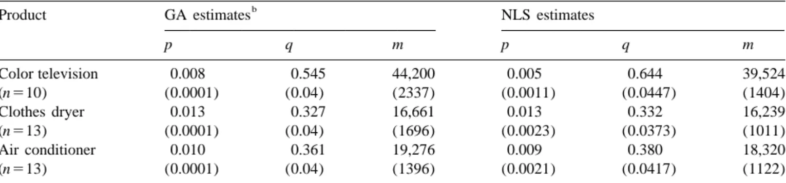
normal distribution, and (2) variance of b¯ The results of this study are outlined in Table
2 2 221
1. As can be seen from this table, estimates 2s
s
d f(x ,t b) / dbd
(Griffiths, Hill, & Judge,obtained from GAs closely replicate the esti-1993). The estimates from GA are reliable if
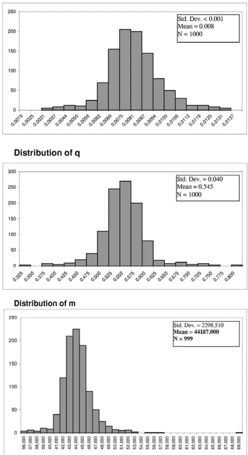
mates from NLS in all the datasets. The dis-they exhibit these properties of estimates from
tribution of parameter estimates from GAs for a non-linear least squares. The investigation of the
sample dataset (color television) is provided in asymptotic properties of the estimates from GA
Fig. 3. The Figure shows that the estimates is important for deriving inferences based on the
obtained from GAs are normally distributed and estimates from GA. If the estimates from GAs
have acceptable standard deviations that are exhibit properties similar to estimates from least
proportional to the asymptotic standard devia-squares, the tests such as t-test, and F-test hold
tions obtained from the NLS method. Thus, it for the estimates of GA also.
can be inferred that the parameter estimates We use the datasets used in Bass et al. (1994)
obtained from GAs are consistent and have the to establish asymptotic properties because these
desirable properties of standard statistical datasets have sales data well after the peak sales
6
techniques . time period. The Monte Carlo simulation is
performed as follows:
4
.3. Predicting future sales
(a) For each dataset the estimation procedure is
repeated 1000 times to obtain a matrix of 4 .3.1. Parameter comparison with simulated
1000 estimates each of p, q, and m for datasets
every dataset, resulting in a total of 3000 Fifty datasets were simulated for the purpose
cells in each matrix. of understanding the performance of GA as
(b) The values of p, q, and m are then plotted compared to NLS and OLS when both full and as a histogram to test for their consistency
and distributional properties. 6
The bias in the parameter estimates can also be checked from the contour plots of the residuals obtained from the
These estimates are then compared with the parameter estimates.
Table 1
a Estimates From GA and NLS for the asymptotic properties study
b
Product GA estimates NLS estimates
p q m p q m Color television 0.008 0.545 44,200 0.005 0.644 39,524 (n510) (0.0001) (0.04) (2337) (0.0011) (0.0447) (1404) Clothes dryer 0.013 0.327 16,661 0.013 0.332 16,239 (n513) (0.0001) (0.04) (1696) (0.0023) (0.0373) (1011) Air conditioner 0.010 0.361 19,276 0.009 0.380 18,320 (n513) (0.0001) (0.04) (1396) (0.0021) (0.0417) (1122) a
The values in parentheses below the reported estimates represent standard errors of the estimates, and n5sample size. b
Table 2
a Reproduction of model parameters: results from the simulation study
True values Full data (sample size T517) Censored dataset (sample size t57)
p q m p q m p q M NLS 0.030 0.380 100 0.026 0.410 972 b b b (0.006) (0.008) (0.027) NA NA NA GA 0.030 0.380 100 0.032 0.370 1015 0.034 0.370 950 (0.003) (0.008) (10.280) (0.003) (0.019) (9.854) a
Reported values are means of the estimates obtained over 50 repeats. Values in parentheses are their respective standard deviations. The peak data point is observed at t510.
b
NA—Not applicable because the estimates are biased.
censored data points are used. The datasets were words closer to the true values) than the esti-mates from NLS ( p50.030, q50.600, m5
simulated using the Srinivasan and Mason
620). (1986) operationalization and a proportional
7
Normal error structure with variance of 0.600 .
The parameter estimates for the simulation 4 .3.2. Comparison of forecasts with simulated
study were set at p*50.030, q*50.380 (mean datasets
estimates reported by Sultan et al. (1990) in In the previous experiment we compared the capability of GA and NLS in reproducing the their meta-analysis of diffusion studies), and
true parameter estimates of p, q, and m from
m*51000. For each of the fifty datasets, the
simulated datasets. We also conducted another diffusion curve was simulated for 17 time
simulation experiment to compare the forecast-periods. On average, the peak for the diffusion
¨ ing ability of GA, NLS, OLS, and a naıve curve occurred around t510. The results of the
8
simulation study are provided in Table 2. As moving average technique . We created a simu-can be seen from Table 2, the estimates from lated dataset from the Bass model with the true GA ( p50.030, q50.370, m51015) are similar parameter estimates of p*50.008, q*50.280, to the estimates obtained from NLS ( p50.026, and m*5100. We added a proportional error
q50.410, m5972) when full datasets are used. variance of 0.600 to the resulting sales data and Also, the estimates from both the techniques generated data up to 20 time periods. We closely resemble the true values ( p*, q*, and censored the datasets at t59 until t519 in
m*) used to simulate the datasets. The datasets order to compare the one-step ahead to eleven-were censored around t57 such that there is no step ahead forecasts from the above four meth-incidence of the peak time period in the cen- ods. Specifically, for the eleven step ahead sored datasets. The estimates from GA ( p5 forecast, we censored the data at t59. Based on 0.034, q50.370, m5950), based on the cen- the estimates from the censored data, we fore-sored datasets, are more accurate (in other cast the rest of the data points (t510 until
t520). The MAE is calculated as the difference
7
We used a variance of 0.600 because this is the commonly found error variance in a majority of empirical datasets.
8
Also, Van den Bulte and Lilien (1997) use a similar error The forecasted sales in next period based on the moving variance in the Monte Carlo simulation regarding diffusion average is calculated as the average sales from the year of data. introduction until the current year.
between the forecasted values and the observed horizons greater than four steps ahead. One values in the holdout sample. For the one-step possible reason for this could be that both NLS, ahead forecasts, the data is first censored at and OLS require the peak time period in order
t59. Based on the estimates from the censored to provide reliable estimates. In other words, dataset, we forecast the sales at t510. The both NLS and OLS required at least 14 data absolute difference between the predicted sales points (with respect to our experiment) to for the next time period, t510 and observed provide reliable estimates. The forecasting sales at t510 is calculated. The above process horizons of five steps ahead or more were is repeated by advancing the censoring point by generated from datasets with less than 13 data one step (i.e., censoring point t510, 11, . . . , points. This is reflected in the poor RAE 19) and calculating the absolute difference measures for NLS and OLS for forecasting between the forecasted values in the next period horizons greater than four steps ahead. Overall, (i.e. t511, 12, . . . , 20) and the observed the estimates from GA are much more reliable values. The mean of the calculated absolute for forecasting sales as compared to NLS, OLS
¨
errors gives the MAE for one step ahead or a naıve moving average method. The simula-forecasts. The above process can be repeated for tion analysis hence establishes the utility of GA two steps ahead and so forth. The peak period in forecasting future sales when the dataset does (t*) in the simulated dataset occurred at the 13th not contain peak sales. In the following analy-time period. The forecasting performance was ses, we investigate the utility of GA in real assessed using the Relative Absolute Error empirical datasets.
(RAE) measure. The results of our experiment are provided in Table 3. As can be seen from
5
. Empirical analyses and validation of Table 3, the forecasts based on GA are clearly
forecasts
better than NLS, OLS or a moving average
measure. The moving average measure performs Sales data on cellular phones in seven west-better than either NLS or OLS for forecasting ern European countries—Norway, Denmark,
Table 3
a Forecasting performance of estimation methods with simulated data
RAE RAE RAE
GA vs. NLS GA vs. OLS GA vs. moving b average
One step ahead 0.697 0.492 0.318
Two step ahead 0.463 0.367 0.304
Three step ahead 0.214 0.261 0.280
Four step ahead 0.112 0.125 0.240
Five step ahead 0.057 0.037 0.169
Six step ahead NA NA 0.133
Seven step ahead NA NA 0.153
Eight step ahead NA NA 0.159
Nine step ahead NA NA 0.133
Ten step ahead NA NA 0.144
Eleven step ahead NA NA 0.029
NA5Reliable estimates were not possible for NLS / OLS. Hence the RAE measure is not applicable. a
The total data length is T520. The peak data point occurs at t513. The censoring of datasets begin at t59 until t519. b
Fig. 4. Diffusion curve for Finland.
representative country (Finland) is provided in Finland, Germany, United Kingdom, France,
Fig. 4. The analysis is performed on both the and Italy, are used to evaluate the forecasting
full datasets and on right censored data sets accuracy of the estimates obtained using GA,
such that the censored data sets do not contain NLS, and OLS on the Bass model and the
the peak period sales but contain enough data estimates from a time-series model. The data
points to obtain reasonable estimates. In other were gathered from published sources such as
words the Bass model can provide estimates
Merchandising Week, Census Reports,
even when only three data points are available. Euromonitor and other trade publications. The
However, the estimates from the Bass model are data obtained from these sources represent the
not robust until data representing the left inflec-number of cellular phone account subscriptions
9
tion point is available in the dataset. Hence, the each year . Data are available from 1981 until
datasets are censored such that the each dataset 2000 for the countries used in this database and
contains data up until the left inflection points. the peak time period ranges from 1993
(Fin-The data points included in each censored land) to 1996 (Italy). The diffusion curve for a
dataset and the point to peak sales is provided in Table 4. The censored datasets can be
consid-9
While it is possible that a given person may open multiple ered as calibration datasets, and the information
accounts with a service provider, it is reasonable to assume available after the censoring time period are that an individual would use only a single cellular phone. used as holdout samples for testing forecasting Relatives or close friends normally use the other accounts.
accuracy. The peak time period reported in the
Hence, the unique nature of the industry allows us to
third column of Table 4 represents the observed
alleviate the problem of replacement purchases associated
Table 4
Censored data lengths and peak time period for cellular adoption
Country Start Peak Censored Holdout a
year year data length
Norway 1981 1994 10 (1981–90) 9 Denmark 1982 1994 9 (1982–90) 9 Finland 1982 1993 7 (1982–88) 11 Germany 1984 1995 8 (1984–91) 8 United Kingdom 1983 1995 9 (1983–91) 8 France 1985 1996 9 (1985–93) 6 Italy 1985 1996 8 (1985–92) 7 a
Values in parentheses represent the years used in the calibration sample.
5
.1. Results from using Bass model on the full and OLS for all the seven datasets analyzed.
and censored datasets When full datasets are used, as revealed in a previous analysis (Table 1), the estimates from The estimates from GA, NLS and OLS were GA, NLS and OLS are similar, except that there obtained based on both the full and censored is a consistent downward bias in the estimates datasets. The estimates from all three techniques of m, from OLS. The above results show that are provided in Tables 5 and 6. With respect to while GA estimates are similar to estimates full datasets, the estimates from GA provide from other techniques, they also provide better better fit (measured in terms of Mean Absolute fit to the data.
Deviation) to the datasets as compared to the With respect to censored datasets, the esti-estimates from NLS and OLS. The mean abso- mates from NLS converge for only two (Nor-lute deviation (MAD) of the estimates from GA way and Denmark) of the seven countries used. is less than the MAD of the estimates from NLS The estimates from OLS make sense for four
Table 5
Estimates from GA and NLS when full datasets are used
a
Country GA estimates NLS estimates OLS estimates
p q m Mean p q m Mean p q m Mean
absolute absolute absolute
error error error
b
(MAE) (MAE) (MAE)
Norway 0.003 0.300 4668 21.26 0.004 0.300 4670 21.26 0.005 0.320 4400 25.17 Denmark 0.004 0.300 3640 11.59 0.003 0.310 3601 12.09 0.006 0.330 3398 13.64 Finland 0.003 0.380 4151 20.68 0.001 0.380 4239 20.68 0.008 0.400 3878 32.60 Germany 0.002 0.440 15 203 96.43 0.0004 0.440 15 217 161.78 0.006 0.500 13 572 148.49 United Kingdom 0.004 0.320 22 771 122.47 0.002 0.330 22 694 128.05 0.010 0.350 20 774 185.11 France 0.003 0.370 8911 29.30 0.001 0.380 8881 31.71 0.008 0.410 7968 45.61 Italy 0.001 0.480 14 033 69.10 0.0002 0.480 14 037 69.46 0.008 0.560 12 209 133.02 a
The reported estimates are means over 50 repeats.
b
The reported MAEs evaluate the in-sample fit and are based on the absolute differences between the predicted values and actual values of the entire data which is also used for estimation (e.g. for Finland, the number of observations is equal to 18 [calibration1holdout]; refer to Table 4 for information on other countries).
Table 6
a Estimates from GA and NLS when censored datasets are used
b
Country GA estimates NLS estimates OLS estimates
p q m Mean p q m Mean p q m Mean
absolute absolute absolute
error error error
c
(MAE) (MAE) (MAE)
Norway 0.005 0.380 1951 225.66 0.005 0.580 1197 250.89 0.009 0.830 757 241.58 Denmark 0.005 0.390 1650 153.64 0.005 0.460 1136 165.17 0.012 0.480 1232 208.21 Finland 0.0004 0.530 8955 420.21 n.c. n.c. n.c. n.p. 0.011 0.770 612 315.20 Germany 0.0008 0.480 17 755 357.30 n.c. n.c. n.c. n.p. n.c. n.c. n.c. n.p. United Kingdom 0.002 0.500 20 000 544.96 n.c. n.c. n.c. n.p. n.c. n.c. n.c. n.p. France 0.004 0.460 2164 706.76 n.c. n.c. n.c. n.p. 0.013 0.740 2435 726.67 Italy 0.0003 0.620 17 120 540.31 n.c. n.c. n.c. n.p. n.c. n.c. n.c. n.p.
n.c.5No convergence was achieved.
n.p.5RAE not possible due to lack of convergence in estimates.
a
The calibration (in other words, the censored data length) and hold-out periods for each country can be obtained from Table 4.
b
The reported estimates are means over 50 repeats.
c
The reported MAEs are based on the absolute differences between the predicted values and actual values of the holdout sample.
(Norway, Denmark, Finland and France) of the performance of GA with censored datasets is seven datasets. For the other three datasets assessed using the Relative Absolute Error (Germany, United Kingdom, and Italy), the (RAE) measure. The RAE between GA, NLS, estimates from OLS do not conform to the and OLS are provided in Table 7. The RAE restrictions of the Bass model, such as 0,q, measure indicates that GA performs better than
p,1 and m.0. However, the estimates from NLS whenever we are able to obtain estimates GA are robust even when censored datasets are from NLS with censored datasets. Also, GA is used. The model fit based on estimates from GA able to provide better forecasts than OLS when on censored datasets is similar to the model fit censored datasets are used.
obtained using full datasets. Also, when com- In order to obtain a clearer picture regarding paring the estimates from GA with the estimates which methodology is superior, we use two from NLS (whenever the NLS algorithm con- other measures that are of interest to practicing verged), the fit of estimates from GA is better managers: the peak time period of sales, and than the fit of the estimates from NLS for both sales during the peak of the product life cycle.
the datasets (Norway5225.6 vs. 250.89, and The time period for peak sales is very critical to Denmark5153.64 vs. 165.17). With respect to product managers because it signifies the end of the performance of GA as compared to OLS, growth phase and the start of the maturity phase the fit of the estimates from GA are better than (i.e., when competition increases and profit the fit of the estimates from OLS for all the decreases). Similarly, sales during the peak of a datasets (Norway5225.6 vs. 241.58, product life cycle indicate the maximum po-Denmark5153.64 vs. 208.21, France5706.76 tential a product can achieve under current vs. 726.67) except Finland (420.21 vs. 315.2). market / firm conditions. This figure also de-The results from this analysis reveal that overall termines the budget for advertising and other the estimates from GA are robust irrespective of marketing expenditures during the growth whether full and censored datasets are used. The phase.
Table 7
Relative absolute error in category sales from various forecasting methods (from censored datasets)
a b c
Country NLS OLS Time series Holdout data d length Norway 0.89 0.93 0.79 9 Denmark 0.93 0.74 0.92 9 Finland N /A 0.73 0.58 11 Germany N /A N /A 0.95 8 United Kingdom N /A N /A 0.4 8 France N /A 0.74 0.83 6 Italy N /A N /A 0.76 7 N /A5Not applicable. a
RAE of predictions from GA versus predictions from NLS. b
RAE of predictions from GA versus predictions from OLS. c
RAE of predictions from GA versus predictions from the time series model. d
RAE values in this table are based on the holdout data which were not used in the estimation of model parameters.
The time to peak sales for a new product mum deviation of the predictions based on GA based on the estimates of the Bass model can be is two time periods (Denmark). It is worth obtained from Eq. (4). The predictions of time mentioning here that whenever unbiased esti-to peak sales based on estimates from GA, NLS mates were obtained from NLS (for Norway and OLS is provided in Table 8. Based on the and Denmark) the predictions of peak time results, we see that overall, GA performs better period from NLS were worse than that provided than both NLS and OLS in predicting the time by GA. In other words, for Norway the predic-to peak sales of a new product. Also, it can be tion based on NLS is off by 6 time periods as seen that GA is able to exactly identify the time compared to 1 time period with the prediction to peak sales in a majority of the datasets based on GA. Similarly, for Denmark, the (Finland, Germany, and Italy). Also, the maxi- prediction based on NLS is off by 3 time periods as compared to 2 time periods for predictions based on GA. The estimates from
Table 8
Predictions of time (years) to peak sales from various OLS perform the worst with respect to
forecast-a
forecasting methods ing the time to peak sales. The predictions based
on OLS are off by at least 6 time periods
Country GA NLS OLS Time
series (Denmark) whenever sensible estimates are
obtained.
Norway 13 (14) 8 (14) 5 (14) 16 (14)
Table 9 compares the forecasted peak period
Denmark 11 (13) 10 (13) 8 (13) 13 (13)
Finland 13 (13) N /A 5 (13) 17 (12) sales from GA, NLS, and OLS. The results from
Germany 13 (12) N /A N /A 12 (12) this analysis also reveal that the Bass model is United Kingdom 11 (10) N /A N /A 12 (10) able to predict the magnitude of sales during the France 13 (12) N /A 5 (13) 13 (12)
peak better than NLS and OLS for all the
Italy 12 (12) N /A N /A 13 (12)
datasets. Specifically, the difference between the
N /A5Not applicable.
predicted peak period sales and the actual peak
a
Value in parenthesis is the actual peak time period in
period sales based on GA ranges from 5 units
years. The predictions for peak are based on estimates
(Denmark) to 184 units (United Kingdom).
from calibration datasets. The calibration data length for
Table 9
a Predictions of peak sales (in ’000s) from various forecasting methods
Country GA NLS OLS Time series
Norway 359 (398) 172.60 (398) 157.98 (398) 443 (398) Denmark 306 (301) 132 (301) 145 (301) 337 (301) Finland 405 (412) N /A 119 (412) 484 (412) Germany 1631 (1601) N /A N /A 1785 (1601) United Kingdom 1717 (1901) N /A N /A 2334 (1901) France 869 (870) N /A 459 (870) 995 (870) Italy 1685 (1621) N /A N /A 1688 (1621) N /A5Not applicable. a
Value in parenthesis is the actual peak sales. The predictions for peak are based on estimates from calibration datasets. The calibration data length for each country is provided in Table 4.
10
NLS (for the two datasets where predictions purposes . The time-series equation for each could be obtained) are 226 units (Norway) and individual country can be represented as: 169 units (Denmark). With respect to the
esti-Dyt5a1b1Dyt21 (7)
mates from OLS the difference in predictions
ranges from 156 units (Denmark) to 411 units where Dyi5first difference of sales of cellular (Finland). Also, for each country the predictions phones in time period i, a5intercept and bs5
based on OLS have the highest difference and slope parameter. We used one-step ahead fore-the predictions based on GAs have fore-the lowest casts to evaluate the forecasting accuracy from difference. These results imply that overall a the Bass model using GA and the time series GA estimation technique is a better option for model, when censored datasets are used. the Bass model during the growth phase of the The results are provided in Fig. 5 for a
product life cycle. representative country (Finland). To obtain the
one-step ahead forecasts, the datasets were re-estimated using GA at every iteration (i.e., as
5
.2. Comparison of results from the Bass
new data points are added). As can be seen
model and a time series model
from Fig. 5, the one-step ahead forecasts from In this section, we compare the forecasting GA track the actual sales of a new product very
¨
capability of the Bass model against a naıve closely. The estimates of p and q, which time series model. In order to design a time- determine the shape of the distribution, do not series forecasting model for the cellular phone change much when new data points are added at dataset, we plotted the autocorrelations for each step of the forecasting process. However, different lags to determine how to generate a
10
stationary series. All the datasets were station- We chose to use an ARIMA (1,1,0) model because the time series model performed better than an exponential
ary with first differences. An examination of the
smoothing or a moving average model. We were able to
partial auto-correlations revealed that an
obtain meaningful autocorrelation functions even when
ARIMA (1,1,0) equation satisfies the sales
there were only 10–15 data points for estimating the
pattern of a majority of the countries. We hence sample values. Examples for finding significant autocorre-adopt an ARIMA (1,1,0) equation of the first lations when lesser number of data points are available can
¨
Fig. 5. One step ahead forecasts for Finland.
the value of the estimate of m does change maximum deviation based on predictions from when new data points are added. The above GA is two time periods (Denmark) as compared pattern is intuitive given that p and q determine to five time periods (Norway) for predictions the shape of the diffusion curve, and hence need from the time series model. Finally, while the
¨
not change with additional information after the naıve time series model performs better than inflection point is reached. However, the value NLS and OLS with respect to predicting the of m provides magnitude to the diffusion curve, magnitude of peak sales it does not compare and the short-term one step ahead forecasts will well with the Bass model estimated using GA. depend on the value of m. It can be inferred Specifically, the difference in predicted peak from Fig. 5 that GA is very useful to managers sales and actual peak sales based on the time to generate short-term one-step ahead forecasts series model is consistently higher than the of sales and long-term forecasts regarding the respective difference based on the predictions
shape of the curve. from GA. In summary, the Bass model
esti-The Bass model estimated using GA also mated using GA is clearly the best option when ¨
fares better than a naıve time series model with long range forecasting is the requirement. For respect to one-step ahead forecasts. The RAE short-term forecasts, researchers should investi-for the Bass model versus the time series model gate the utility of a combination of forecasts
¨
is lower (less than one) for all the countries from the Bass model and a naıve time series analyzed (as shown in Table 7). However, the model.
5
.2.1. Future forecasts market is a long-term phenomenon. The
fore-In this section we provide forecasts of future casts based on GA suggest that the sales of sales of cellular phones (over a two year cellular phones are (1) expected to grow only in horizon) in the seven countries studied. The Norway, (2) the sales have reached a stationary results of this forecasting exercise are provided state in Finland and Denmark, and (3) the sales in Fig. 6. As indicated in Fig. 6a, the sales of is expected to slowdown in France, UK, Italy, cellular phones seem to have stabilized for and Germany. The results indicate that overall Finland and Denmark. The prospects for growth the growth rate for cellular phones is reaching are high only for Norway, while the sales of maturity and that firms should focus on newer cellular phones are predicted to decline for and useful innovations if they need to sustain Germany, UK, Italy, and Denmark. Overall, the their current growth rate and profit margins. telecommunications industry seems to have The forecast of wireless subscribers in our stabilized and high growth rates as observed in study was accomplished by estimating the the past may not be experienced in the future. Srinivasan and Mason (1986) operationalization Also, there doesn’t seem to be any drastic of the Bass diffusion model using GA. The changes in the diffusion trend for the future results from our analyses using GA are very sales. The results of our analyses also imply that encouraging to both practitioners and research-the forecasts of sustained growth in research-the tele- ers alike. It is found that the predictions from communications industry need to be qualified. GA are robust across many datasets and are better than OLS and NLS with respect to both Relative Absolute Error (RAE) and predictions of time to peak sales, when forecasting is done
6
. Conclusions and future research
in the growth phase and the maturity phase of In this study we address the issue of forecast- product life cycle. The Bass model estimated
¨ ing sales in dynamic and turbulent markets such using GA also performed better than a naıve as the telecommunications sector. Specifically time series model (Eq. (7)). The estimates during the growth phase, volatility with respect generated from a GA also have desirable prop-to price, new product offerings and competiprop-tor erties such as (1) a normal distribution and (2) actions, and entry of new brands (as evident in bounded variance.
the telecommunication sector) make predicting Future research studies can investigate the future sales, time to peak sales and magnitude utility of including several exogenous factors of peak sales a non-trivial task for product such as price, competitive intensity, and net-managers. The current slowdown in growth in work effects in obtaining better predictions the telecommunications sector makes such a during the growth phase. The recent phase of study of critical importance. In order to achieve consolidation in the telecommunications indus-this objective we propose a simulation based try could provide avenues to investigate how the search technique for estimating the Bass model competitive intensity, measured in terms of and illustrate our algorithm by providing predic- market share concentration or price volatility, tions of category sales, time of peak sales, and influences the diffusion of new products and sales at the peak, of cellular phones in seven telecommunications equipment in particular. countries during the growth phase of its life Also, the telecommunication industry is depen-cycle. The results suggest that in the seven dent to a large extent on network externalities European countries in our study the current such as high bandwidth for better communica-slowdown in growth in the wireless phones tion facilities and hence higher rates and levels
Bass Model fits without decision variables. Marketing
of adoption. The above examples illustrate some
Science,3, 203–223.
representative theoretical and managerial issues
Bayus, B. L. (1992). The dynamic pricing of next
gene-that need to be resolved in the telecommunica- ration consumer durables. Marketing Science, 11(3), tions sector related to product / service adoption. 251–266.
The technique proposed in this study can be Bowerman, B. L., & O’Connell, R. T. (1993). Forecasting
and Time Series: An Applied Approach, 3rd ed..
Bel-used as a basis for further investigation of
mont, California: DuxBury Press.
product adoption in nascent markets.
Research-Fildes, R. (2002). Telecommunications demand
forecast-ers should also investigate the applicability of
ing—a review. International Journal of Forecasting,
these results across different product categories, 18.
especially those that have different product Ganesh, J., Kumar, V., & Subramanian, V. (1997). Learning
market characteristics such as High Definition effect in multinational diffusion of consumer durables: an exploratory investigation. Journal of the Academy of
Televisions. In this study, we investigate only
Marketing Science., 25(3), 214–228.
one aspect of the drawbacks in using NLS for
Goldberg, D. E. (1989). In A Simple Genetic Algorithm in
estimating the Bass model. The issue of
sys-Genetic Algorithms in Search Optimization and Ma-tematic change and bias in parameter estimates chine Learning. Addison Wesley Longman, pp. 10–14. of the Bass model when using NLS still needs Griffiths, W. E., Hill, R. C., & Judge, G. G. (1993).
Learning and Practicing Econometrics. New York: John to be investigated. GAs could very well serve as
Wiley & Sons.
an alternative estimation technique under this
Hyman, M. R. (1988). The timeliness problem in the
scenario.
application of Bass-type new product growth models to
Of primary interest however, would be to durable sales forecasting. Journal of Business Research, investigate the performance of GAs compared 16(1), 31–47.
to newer techniques such as Hierarchical Bayes, Jamieson, L. F., & Bass, F. M. (1989). Adjusting stated intention measures to predict trial purchase. Journal of
Kalman filtering, and any combinations of these
Marketing Research,26(3), 336–346.
methods. Also, research is needed on deriving
Jain, D. C., & Rao, R. C. (1990). Effect of price on the
algorithms to combine the forecasts from these demand for durables: modeling, estimation, and find-different techniques. ings. Journal of Business and Economic Statistics, 8,
163–170.
Kumar, V., & Krishnan, T. V. (2002). Multinational diffu-sion models: an alternative framework for modeling A
cknowledgements
cross-national diffusion. Marketing Science, 21(3), 318–330.
The authors thank the editor-in-chief, the Lawrence, K. D., & Lawton, W. H. (1981). Application of reviewers, Frank M. Bass, Trichy V. Krishnan, diffusion models: some empirical results. In Wind, Y., Robert P. Leone, and Srini Srinivasan for their Mahajan, V., & Cardozo, R. C. (Eds.), New Product
Forecasting. Lexington, MA: Lexington Books, pp. comments on earlier versions of this paper.
529–541.
Lenk, P. J., & Rao, A. G. (1990). New models from old forecasting product adoption by hierarchical Bayes R
eferences procedures. Marketing Science,9, 42–53.
Mahajan, V., Muller, E., & Bass, F. M. (1990). New Bass, F. M. (1969). A new product growth model for product diffusion models in marketing in: a review and consumer durables. Management Science,15, 215–227. directions for future research. Journal of Marketing, Bass, F. M. (1980). The relationship between diffusion 54(1), 1–26.
rates, experience curves, and demand elasticities for Mahajan, V., & Sharma, S. (1986). A simple algebraic consumer durable technological innovations. Journal of estimation procedure for innovation diffusion models of
Business,53, 51–67. new product acceptance. Technological Forecasting and Bass, F. M., Krishnan, T. V., & Jain, D. (1994). Why the Social Change, 30, 331–345.
Meade, N., & Islam, T. (2001). Forecasting the diffusion Biographies: V. KUMAR (VK) is the ING Chair of innovations for time-series extrapolation. In Am- Professor of Marketing, and Executive Director, ING strong, S. (Ed.), Principles of Forecasting: A Handbook Center for Financial Services in the School of Business,
for Researchers and Practitioners. Boston: Kluwer University of Connecticut. He has been recognized with Academic Publishers, pp. 577–596. many teaching and research excellence awards and has Modis, T., & Debecker, D. (1992). Chaoslike states can be published numerous articles in many scholarly journals in expected before and after logistic growth. Technological marketing including the Harvard Business Review, Journal
Forecasting and Social Change,41, 111–120. of Marketing, Journal of Marketing Research, Marketing Kalish, S. (1983). Monopolistic pricing with dynamic Science, and Operations Research. He has co-authored demand and production cost. Marketing Science, 2, multiple textbooks on Marketing Research. His interest in 135–160. International and Forecasting area is very well reflected by Kotler, P. (2000). Marketing Management. Prentice Hall. his research publications in many major journals including Krishnan, T. V., Bass, F. M., & Kumar, V. (2000). Impact the International Journal of Forecasting, Journal of of a late entrant on the diffusion of a new product or International Marketing, International Journal of Re-service. Journal of Marketing Research, 269–278. search in Marketing, and the Journal of World Business.
Kumar, V., Ganesh, J., & Echambadi, R. (1998). Cross- He has authored a book titled International Marketing national diffusion research: what do we know and how Research, which is based on his marketing research
certain are we? Journal of Product Innovation Manage- experience across the globe. He is on the editorial review
ment,15, 225–268. board of many scholarly journals and has lectured on Parker, Philip M. (1994). Aggregate diffusion forecasting marketing-related topics in various universities and organi-models in marketing: a critical review. International zations worldwide. His current research focuses on
interna-Journal of Forecasting,10, 353–381. tional diffusion models, customer relationship manage-Robinson, B., & Lakhani, C. (1975). Dynamic price ment, customer lifetime value analysis, sales and market models for new product planning. Management Science, share forecasting, international marketing research and 10, 1113–1122. strategy, coupon promotions, and market orientation. He Schmittlein, D. C., & Mahajan, V. (1982). A maximum served on the Academic Council of the AMA as a Senior likelihood estimation for an innovation diffusion model V.P. for Conferences and Research and a Senior V.P. for of new product acceptance. Marketing Science,1, 57– International Activities. He was recently listed as one of 78. the top fifteen scholars in marketing worldwide. He is a Seber, G. A. F., & Wild, C. J. (1993). Nonlinear Regres- consultant for many Fortune 500 firms and has also
sion. New York: John Wiley. worked with these companies’ databases to identify profit-Srinivasan, V., & Mason, C. H. (1986). Nonlinear least able customers. He received his Ph.D. from the University
squares estimation of new product diffusion models. of Texas at Austin.
Marketing Science,5(2), 169–178.
Sultan, F., Farley, J. U., & Lehnmann, D. R. (1990). A meta-analysis of diffusion models. Journal of Marketing
Research,27, 70–77. Rajkumar VENKATESAN is Assistant Professor of
Takada, H., & Jain, D. C. (1991). Cross-national analysis Marketing at the University of Connecticut. He has a of diffusion of consumer durable goods in Pacific Rim Bachelors degree in Computer Science and Engineering countries. Journal of Marketing,55, 48–54. from University of Madras. Raj’s research interests include Van den Bulte, C., & Lilien, G. L. (1997). Bias and Customer Relationship Management, Customer equity vs. systematic change in the parameter estimates of macro firm value, E-Business models, and new product innova-level diffusion models. Marketing Science, 16(70), tions. He is the winner of the 2001 Alden G. Clayton 338–353. Dissertation Proposal award from the Marketing Science
Venkatesan, R., Krishnan, T.V., & Kumar, V. (2001). Institute, the 2001 ISBM Doctoral Dissertation competition Structural Asymmetry and Consistent Estimation of Outstanding Submission award and the Best Track Paper
Macro-level Diffusion Models. Working Paper, Uni- Award in the 1999 American Marketing Association