1
The Impact of Response Shift on the Assessment of Change: Calculation of Effect-Size Indices Using Structural Equation Modeling
Verdam1,2, M.G.E., Oort2, F.J., Sprangers1, M.A.G.
1.
Academic Medical Centre/University of Amsterdam
2.
Child Development and Education, University of Amsterdam
Correspondence concerning this article should be addressed to M.G.E. Verdam, Department
2 Abstract
Objective. The investigation of response shift in patient-reported outcomes (PROs) is important in both clinical practice and research. Insight into the presence and strength of response shift effects is necessary for a valid interpretation of change.
Study Design and Setting. When response shift is investigated through structural equation modeling (SEM), observed change can be decomposed into: 1) change due to recalibration response shift, 2) change due to reprioritization and/or reconceptualization response shift, and 3) change due to change in the construct of interest. Subsequently, calculating effect-size indices of change enables evaluation and interpretation of the clinical significance of these different types of change.
Results. Change was investigated in health-related quality of life data from 170 cancer patients, assessed prior to surgery and three months following surgery. Results indicated that patients deteriorated on general physical health and general fitness, and improved on general mental health. The decomposition of change showed that the impact of response shift on the assessment of change was small.
Conclusion. SEM can be used to enable the evaluation and interpretation of the impact of response shift effects on the assessment of change, particularly through calculation of effect-size indices. Insight into the occurrence and clinical significance of possible response shift effects will help to better understand changes in PROs.
Keywords: effect size; clinical significance; patient-reported outcomes; health-related quality of life; structural equation modeling; change assessment.
Running Title: Calculation of effect-size indices of change.
3 Key findings
In this paper we explain how the impact of response shift on the assessment of change can be
evaluated through the calculation of effect-size indices of change in order to convey information about the clinical meaningfulness of results.
What this adds to what is known
Structural equation modeling provides a valuable tool for the assessment of change, and
investigation of response shift in patient-reported outcomes. The decomposition of change – and subsequent calculation of effect-size indices – provides insight into the impact of
response shifts on the assessment of change.
What is the implication, what should change now
Advancing the standard reporting of effect-size indices of change will enhance the
comparison of effects, facilitate future meta-analysis, and provides insight into the size of the
4 Introduction
Patient-reported outcomes (PROs) have become increasingly important, both in clinical
research and practice. PROs may include measures of subjective wellbeing, functional status, symptoms, or health-related quality of life (HRQL). The patient perspective on health
provides insight into the effects of treatment and disease that is imperative for understanding health outcomes. PROs thus present important measures for evaluating the effectiveness of treatments and changes in disease trajectory, especially in chronic disease (Revicki, Hays,
Cella, & Sloan, 2008), and palliative care (Ferrans, 2007).
The investigation and interpretation of change in PROs can be hampered because
different types of change may occur. Differences in the scores of PROs are usually taken to indicate change in the construct that the PROs aim to measure. However, these differences can also occur because patients change the meaning of their self-evaluation. Sprangers &
Schwartz (1999) proposed a theoretical model for change in the meaning of self-evaluations, referred to as ‘response shift’. They distinguish three different types of response shift:
recalibration refers to a change in respondents’ internal standards of measurements;
reprioritization refers to a change in respondents’ values regarding the relative importance of subdomains; and reconceptualization refers to a change in the meaning of the target construct.
To illustrate, when a patient is being asked to fill in a questionnaire about quality of life, he or she may indicate to be limited in social functioning ‘very often’ before treatment, and ‘some
of the time’ after treatment. The change in these responses can be interpreted as a reduction in social functioning, and indicative of a reduction in quality of life. However, the observed change may also occur because the patient has recalibrated what ‘very often’ means, e.g. the
response ‘very often’ may refer to many more times after treatment than it did before treatment. With reprioritization response shift, the observed change may occur because the
5
with reconceptualization response shift the meaning of a patient’s response may have changed, e.g., a patient may interpret ‘social functioning’ as work-related before treatment,
and as family-related after treatment.
As the occurrence of response shift may impact the assessment of change, the detection
of possible response shift effects is important for the interpretation of change in PROs. One of the methods that can be used to investigate the occurrence of response shift is Oort’s structural equation modeling (SEM) approach (Oort, 2005). Advantages of the SEM
approach are that it enables the operationalization and detection of the different types of response shift, and that it can be used to investigate change in the construct of interest (e.g.,
HRQL) while taking possible response shifts into account. We note, however, that SEM is a group level analysis and will only detect response shifts that affect a substantial part of the sample.
Although clinicians and researchers acknowledge the occurrence of response shift, little is known about the magnitude and clinical significance of those effects (Schwartz et al.,
2006). The detection of response shift is usually guided by tests of statistical significance. Although statistical tests can be used to determine whether occurrences of response shift are statistically significant, they cannot be taken to imply that the result is also clinically
significant (i.e., meaningful). Statistical significance tests protect us from interpreting effects as being ‘real’ when they could in fact result from random error fluctuations. However,
statistical significance tests do not protect us from interpreting small, but trivial effects as being meaningful. Therefore, assessing the meaningfulness of change in PROs has been an important research focus (Cappelleri & Bushmakin, 2014; Sloan, Cella, & Hays, 2005), as it
is imperative for translating results to patients, clinicians or health practitioners. However, there is no universally accepted approach to determine the meaningfulness of change in PROs
6
One of the approaches that can be used to determine the clinical significance of change in PROs is to calculate distribution-based effect-size indices. Distribution-based effect sizes
are calculated by comparing the change in outcome to a measure of the variability (e.g., a standard deviation). The resulting effect sizes are thus standardized measures of the relative
size of effects. They facilitate comparison of effects from different studies, particularly when outcomes are measured on unfamiliar or arbitrary scales (Coe, 2002). In addition, previous research has shown that distribution-based indices often lead to similar conclusions as when
the clinical significance of effects is directly linked to patients’ or clinicians’ perspectives on the importance of change, i.e. so-called anchor-based indices of effects (Cella, et al., 2002;
Eton, et al., 2004; Jayadevappa, Malkowicz, Wittink, Wein, & Chhatre, 2012). Furthermore, the interpretation of effect-size indices as indicating ‘small’, ‘medium’, or ‘large’ effects is possible using general ‘rules of thumb’ (e.g., Cohen, 1988). Therefore, distribution-based
effect-size indices can be used to convey information about the clinical meaningfulness of results.
The aim of this paper is to explain the calculation of effect-size indices within the SEM framework for the investigation and interpretation of change. In addition, we explain how this enables the evaluation and interpretation of the impact of response shift on the assessment of
change. Specifically, we use SEM to decompose observed change into change due to
response shift, and change due to the construct of interest (i.e., ‘true’ change). Subsequently,
we illustrate the calculation and interpretation of various effect-size indices, i.e. the
standardized mean difference, the standardized response mean, the probability of benefit, the probability of net benefit, and the number needed to treat to benefit, for each component of
the decomposition. This enables the evaluation of the contributions of response shift and true change to the overall assessment of change in the observed variables. To illustrate, we will
7
prior to surgery and three months following surgery. We aim to show that distribution-based effect-size indices can contribute to the clinical interpretability of change in PROs.
Method
Calculation of effect-size indices of change
Below we explain the calculation and interpretation of different effect-size indices of change using pre- and post-test comparison as an example. A more detailed explanation of the
(statistical) derivations of these effect-size indices and their interrelationships are offered in an online Technical Appendix.
Standardized mean difference (SMD). One of the distribution-based methods to
describe the magnitude of change, is to express the difference between pre- and post-test means in standard deviation units. The resulting standardized mean difference (SMD) can be
calculated using the standard deviation of the pre-test (see Table 1). This effect size thus expresses the magnitude of change in terms of variability between subjects at baseline, i.e. before the start of treatment. The advantage of using the pre-test standard deviation as a
standardizer is that it is not yet affected by the occurrences between pre-and post-test (Kazis, Anderson, & Meenan, 1989). Although other options for the calculation of the SMD effect
size exist (see A.1 of the Technical Appendix for more details), the pre-test standard
deviation seems to be used most often in the literature (e.g., Copay, Subach, Glassman, Polly, & Schuler, 2007; Durlak, 2009; Hojat & Xu, 2004; Norman, Wyrwich, & Patrick, 2007;
Schwartz, et al., 2006). Therefore, we refer to the resulting effect size as the SMD effect size (see Table 1).
8
index of change (p. 48), as it specifically takes into account the correlation between pre- and post-test assessments (see Table 1).The resulting effect size is known as the standardized
response mean (SRM). It expresses the magnitude of change in terms of between-subject variability in change, which has been argued to be most intuitive and relevant for the
interpretation of effects (Liang, Fossel, & Larson, 1990). Moreover, using the standard deviation of the difference as a standardizer results in an estimate that is equivalent to a z-value, and thus facilitates the translation to other effect sizes (see Table 1). Therefore, in this
9 Table 1
Calculation of effect-size indices of change
ªwhere Φ is the cumulative standard normal distribution.
Interpretation of SMD and SRM effect sizes. As a general rule of thumb, values of 0.2, 0.5, and 0.8 of the SMD effect size can be interpreted as indicating ‘small’, ‘medium’, and
‘large’ effects respectively (Cohen, 1988). It has been argued that application of these rules of thumb for the interpretation of the SRM effect size of change may lead to over- or
under-estimation of effects (Middel & van Sonderen, 2002). Specifically, the interpretation of the SRM effect size of change according to the general rules of thumb may lead to an
underestimation when the correlation between pre- and post-test measurements is smaller
than 0.5, and to an overestimation when the correlation between measurements is larger than 0.5 (see A.2 of the Technical Appendix for more details). However, as it might not be an
unrealistic assumption that correlations between consecutive measurements are generally around 0.5, the rules of thumb for interpretation of the SRM effect size can be applied without a major risk of over- or under-valuation of the magnitude of effects.
Relation to other effect-size indices of change
Effect size Calculation
Standardized mean difference (SMD) 𝑋𝑋�𝑝𝑝𝑝𝑝𝑝𝑝𝑝𝑝−𝑋𝑋�𝑝𝑝𝑝𝑝𝑝𝑝 𝑠𝑠𝑠𝑠𝑝𝑝𝑝𝑝𝑝𝑝
Standardized response mean (SRM) 𝑋𝑋�𝑝𝑝𝑝𝑝𝑝𝑝𝑝𝑝−𝑋𝑋�𝑝𝑝𝑝𝑝𝑝𝑝
�𝑠𝑠𝑠𝑠𝑝𝑝𝑝𝑝𝑝𝑝𝑝𝑝2 + 𝑠𝑠𝑠𝑠𝑝𝑝𝑝𝑝𝑝𝑝2 − 2𝑟𝑟𝑝𝑝𝑝𝑝𝑝𝑝𝑝𝑝,𝑝𝑝𝑝𝑝𝑝𝑝 𝑠𝑠𝑠𝑠𝑝𝑝𝑝𝑝𝑝𝑝𝑝𝑝𝑠𝑠𝑠𝑠𝑝𝑝𝑝𝑝𝑝𝑝
Probability benefit (BP) Φ(SRM)ª
Probability net benefit (PNB) Φ(SRM) – (1 – Φ(SRM)) = 2Φ(SRM) – 1
Number needed to treat to benefit (NNTB) 1
10
The SRM effect-size indices of change express the magnitude of change in terms of standard deviation units. To enhance clinical interpretability of the proposed effect-size index of
change, we explain how this effect size can be converted into other well-known effect-size indices that have been proposed specifically for their intuitive (clinical) appeal.
Probability of benefit (PB). To enhance the interpretability of the magnitude of an effect, it has been proposed to use an estimate of the probability of a superior outcome (Grissom, 1994). In the context of pre- and post-test comparison this refers to the probability
that a random subject shows a superior post-test score as compared to the pre-test score, i.e. the probability that a random subject shows a positive change or improvement over time. We
refer to this effect size as the probability of benefit (PB), but it is also known as the probability of superiority (PS; Grissom, 1994), the common language effect size (CLES; McGraw & Wong, 1992) and the area under the curve (AUC). The effect size was proposed
specifically for its intuitive appeal and ease of interpretation, and has been recommended for developing insights about differences (Kraemer & Kupfer, 2006). The PB effect size can be
calculated using the SRM effect size (see Table 1).
Probability of net benefit (BNP). The PB effect size does not take into account possible detrimental effects. That is, subjects may show a deterioration over time. The effect size that
we refer to as the probability of net benefit (PNB; see Table 1) is the difference between the probability that a random subject improves over time (i.e., PB) , and the probability that a
random subject deteriorates over time (i.e., 1 – PB). Or, in other words, the net probability that a random subject improves over time. This effect size is commonly applied to binary outcomes (e.g. success/failure), where it is known as the success rate difference (SRD;
Rosenthal & Rubin, 1982), absolute risk reduction (ARR), or risk difference (RD). It is one of the effect sizes that is recommended by the consolidated standards of reporting trials
11
Number needed to treat to benefit (NNTB). Another effect size that has been
recommended for clinical interpretability (Kraemer & Kupfer, 2006) is the number needed to
treat (NNT; Laupacis, Sackett, & Roberts, 1988). In the context of pre- and post-test
comparison, the NNT can be interpreted as the expected number of patients that needs to be
treated to have one more patient show an improvement (i.e., benefit) as compared to the expected number of patients who show a deterioration. We refer to this effect size as the number needed to treat to benefit (NNTB; see Table 1), as it is calculated by taking the
inverse of the PNB effect size. It facilitates interpretation of effects in – clinically meaningful – terms of patients who need to be treated to reach a success rather than probabilities of a
success (Sedgwick, 2015). When the net effect is negative (i.e., more patients show a
deterioration as compared to an improvement), then the NNTB is interpreted as the expected number of patients that needs to be treated to have one more patient show a deterioration as
compared to an improvement.
Relation between different effect-size indices of change. The relation between the SRM
and the other effect-size indices of change (i.e., PB, PNB, and NNTB) can be used to derive the respective values of these effect-size indices that correspond to different values of the SRM effect size, including the 0.20, 0.50 and 0.80 thresholds for interpretation of ‘small’,
‘medium’ and ‘large’ effects respectively (see A.3 of the Technical Appendix). For example, a medium SRM effect size corresponds to a PB effect size that indicates that 69% of patients
show an improvement (i.e., PB = 0.69), where 38% more patients show an improvement as compared to a deterioration (PNB = 0.38), and three patients need to be treated to have one more patient show an improvement as compared to the number of expected patients who
show a deterioration (NNTB = 2.61), i.e. for every three patients who are treated two patients will improve as compared to one patient who deteriorates.
12
Within the SEM approach as proposed by Oort (2005), the different response shifts are operationalized by differences in model parameters. Specifically, changes in the pattern of
common factor loadings are indicative of reconceptualization response shift, changes in the values of the common factor loadings are indicative of reprioritization response shift, and
changes in the intercepts are indicative of recalibration response shift. 1 Changes in the means of the underlying factors are indicative of ‘true’ change, i.e., change in the underlying
common factor. The contributions of the different types of response shifts and ‘true’ change
to the changes in the observed variables (i.e., observed questionnaire scores) can be
investigated using the decomposition of change (see A.4 of the Technical Appendix for more
details). Subsequently, using the same standard deviation to standardize observed change, and the different elements of the decomposition, enables evaluation and interpretation of the contribution of recalibration, reprioritization and reconceptualization, and ‘true’ change, to
the change in the observed variables. In addition, the overall impact of response shift on the assessment of change in the underlying construct of interest can be evaluated through the
comparison of effect-size indices for change in the means of the underlying common factors before and after taking into account possible response shift effects.
Illustrative Example
To illustrate the calculation and interpretation of effect-size indices of change we used health-related quality of life (HRQL) data from 170 newly diagnosed cancer patients’. Patients’ HRQL was assessed prior to surgery (pre-test) and three months following surgery
(post-test). The sample included 29 lung cancer patients undergoing either lobectomy or pneumectomy, 43 pancreatic cancer patients undergoing pylorus-preserving
1
13
pancreaticoduodenectomy, 46 esophageal cancer patients undergoing either transhiatal or transthoracic resection and 52 cervical cancer patients undergoing hysterectomy. These data
have been used before to investigate response shift, and details about the study procedure, patient-characteristics and measurement instruments can be found elsewhere (Visser et al.,
2013; Visser, Oort, & Sprangers, 2005; Verdam, Oort, Visser, & Sprangers, 2012). Measures
HRQL was assessed using the SF-36 health survey (Ware et al., 1993) and the
multidimensional fatigue inventory (Smets, Garssen, Bonke, & de Haes, 1995), resulting in the following nine scales: physical functioning (PF), role limitations due to physical health
(role-physical, RP), bodily pain (BP), general health perceptions (GH), vitality (VT), social functioning (SF), role limitations due to emotional problems (role-emotional, RE), mental health (MH), and fatigue (FT). For computational convenience the scale scores were
transformed so that they all ranged from 0 to 5, with higher scores indicating better health. Measurement model
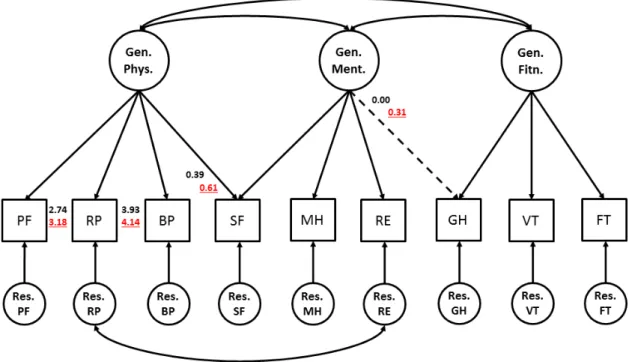
The measurement model is depicted in Figure 1 (see Oort, Visser, & Sprangers, 2005 for more information on selection of this measurement model). The circles represent unobserved, latent variables and the squares represent the observed variables. Three latent variables are
the common factors general physical health (GenPhys), general mental health (GenMent), and general fitness (GenFitn). GenPhys is measured by PF, RP, BP and SF, GenMent is
measured by MH, RE, and again SF, and GenFitn is measured by VT, GH, and FT. Other latent variables are the residual factors ResPF, ResRP, ResBP, etc. The residual factors represent all that is specific to PF, RP, BP, etc., plus random error variation.
The measurement model was the basis for a structural equation model for pre-, and post-test with no across measurement constraints. Imposition of equality constraints on all
14
shift (see Verdam et al., 2012 for more information). Four cases of response shift were identified: reconceptualization of GH, reprioritization of SF as an indicator of GenPhys, and
recalibration of RP and BP (see Figure 1).
Figure 1. The measurement model used in response shift detection.
Notes: Circles represent latent variables (common and residual factors) and squares represent observed variables
(the subscales of the HRQL questionnaires). Numbers are maximum likelihood estimates of the model parameters associated with response shift: common factor loadings (reprioritization and reconceptualization), and intercepts (recalibration). Values represent different pre-test (black) and post-test (red) estimates. These values are taken from Verdam, Oort, & Sprangers (2012) and differ slightly from the results of Oort, Visser & Sprangers (2005) because the former study also included the then-test assessment in the model.
Effect-size indices of change
The parameter estimates of the model in which all response shifts were taken into account
15
General Physical Health. There was an overall medium deterioration in GenPhys (standardized response mean (SRM) = -0.72). Conversion of this effect-size into probability
of benefit (PB), the probability of net benefit (PNB), and the number needed to treat to benefit (NNTB) yielded values of 0.23, -0.53, and -1.88 respectively. This indicates that only
23% of patients showed an improvement over time (PB = 0.23), and that 53% more patients deteriorated than improved (PNB = -0.53). The NNTB indicates that with every 1.88 patients to be treated, there would be one more patient who shows a deterioration as compared to an
improvement. In other words, two of every three patients who are treated are expected to show a deterioration.
The contribution of ‘true’ change (i.e., the change in the observed indicators that is due to change in the underlying common factors) was in the same direction and of similar
magnitude for the indicators that load only on GenPhys (i.e., RF, RP and BP; see Table 2).
The indicator SF loaded not only on GenPhys but also on GenMent, and therefore showed a deviating pattern of change. The contribution of ‘true’ change in this indicator was a
combination of the deterioration of GenPhys and improvement of GenMent (see below), that cancelled each other out.
Three different response shifts were detected for the indicators of GenPhys. Patients’
SF became more important to the measurement of GenPhys after treatment (with a
contribution to change: SRM = -0.10). In addition, patients scored higher on RP and BP after
treatment, as compared to the other indicators of GenPhys (with a contribution to change: SRM = 0.19, and SRM = 0.17 respectively). These occurrences of response shift thus had small effects on the change in the observed indicators. To illustrate, the response shift effect
of BP can be translated as follows (see Table 2): 57% of patients showed a relative improvement (PB = 0.57), with 14% more patients showing a relative improvement as
16
there would be one more patient who shows a relative improvement due to recalibration response shift (NNTB = 7.21), i.e. four patients would show a relative improvement as
compared to three patients who are expected to show a relative deterioration.
The influence of response shift on the assessment of change is apparent when we look
at the estimated effect sizes for observed change. Here, we can see that the deterioration in RP and BP became somewhat smaller as was expected from only the change in GenPhys. In addition, the observed change in SF was slightly more negative, than what would be expected
only from the changes in the underlying factors of GenPhys and GenMent. For the indicator PF there was no response shift detected, and thus the observed change was equal to the
contribution of ‘true’ change (i.e., the observed change in the indicator could be ascribed to change in GenPhys). If response shift had not been taken into account, the change in the underlying common factor GenPhys would have been estimated to be slightly smaller (SRM
= -0.59, instead of SRM = -0.72).
General Mental Health. There was an overall small improvement in GenMent (SRM =
0.48; PB = 0.69; PNB = 0.37; NNTB = 2.69). The contribution of ‘true’ change in the indicators that load only on GenMent (MH and RE) was in the same direction and of similar magnitude (see Table 2). There were no response shifts detected for these indicators, and thus
all observed change could be described to ‘true’ change.
Reconceptualization was detected for the indicator GH, which became indicative of
GenMent after treatment. The contribution of ‘true’ change in the decomposition of change for GH showed a small deterioration (SRM = -0.15), reflecting not only the contribution of ‘true’ change (deterioration) in GenFitn (see below), but also the contribution of ‘true’
change (improvement) in GenMent. The observed change in GH was thus less negative than what would be expected only due to ‘true’ change in GenFitn. This contribution of
17
explains the deviating pattern of observed change in de indicator GH (SRM = -.01). Although the detected response shift had a small impact on the assessment of change at the level of the
indicator, it did not influence the overall change in the underlying common factor GenMent. If response shifts had not been taken into account, the change in GenMent would have been
estimated to be of similar magnitude (SRM = 0.45 instead of SRM = 0.48).
General Fitness. There was an overall small deterioration of GenFitn (SRM = -0.37; PB = 0.35; PNB = -0.29; NNTB = -3.44). The two indicators (VT and FT) that loaded only on
GenFitn showed a deterioration in the same direction and with similar magnitude. There was no response shift detected for these indicators, and thus the observed change in these
18 Table 2
Effect-size indices of (contributions to) change for the decomposition of change
Notes: n = 170; SRM = standardized response mean, where values of 0.2, 0.5, and 0.8 indicate small, medium,
and large effects; PB = probability of benefit; PNB = probability of net benefit, NNTB = number needed to treat
to benefit. a = recalibration, b = reprioritization, c = reconceptualization.
Scale SRM PB PNB NNTB
Observed change
PF -0.51 0.30 -0.39 -2.54
RP -0.28 0.39 -0.22 -4.61
BP -0.25 0.40 -0.19 -5.16
SF -0.09 0.46 -0.07 -13.73
MH 0.37 0.64 0.29 3.49
RE 0.26 0.60 0.21 4.85
GH -0.01 0.49 -0.01 -97.85
VT -0.31 0.38 -0.25 -4.06
FT -0.32 0.37 -0.25 -3.94
Response shift
PF - - - -
RP 0.19a 0.58 0.15 6.51
BP 0.17a 0.57 0.14 7.21
SF -0.10b 0.46 -0.08 -12.56
MH - - - -
RE - - - -
GH 0.14c 0.55 0.11 9.14
VT - - - -
FT - - - -
True Change
PF -0.51 0.30 -0.39 -2.54
RP -0.47 0.32 -0.36 -2.77
BP -0.42 0.34 -0.33 -3.07
SF 0.01 0.50 0.01 159.57
MH 0.37 0.64 0.29 3.49
RE 0.26 0.60 0.21 4.85
GH -0.15 0.44 -0.12 -8.36
VT -0.31 0.38 -0.25 -4.06
19 Discussion
In this paper we have shown how to calculate effect-size indices of change using structural
equation modeling (SEM). We used SEM for the decomposition of change, where observed change (e.g., change in the subscales of a health-related quality of life (HRQL) questionnaire)
is decomposed into change due to recalibration, reprioritization and reconceptualization, and ‘true’ change in the underlying construct (e.g., HRQL). Calculation of effect-size indices for each of the different elements of the decomposition enables the evaluation and interpretation
of the impact of response shift on the assessment of change.
We used distribution-based effect sizes to interpret and evaluate the magnitude of
change, and the impact of response shift on the assessment of change. Specifically, we proposed to use the standardized response mean as the preferred effect size of change. Results from our illustrative example indicated that patients experienced small to medium
sized changes in their scores on the subscales of the HRQL questionnaires. Four response shifts were detected, but the impact of the detected response shift on the assessment of
change was small; both at the level of the observed variables and at the level of the underlying common factors. Similar sizes of effects were reported in a meta-analysis on response shift (Schwartz et al., 2006), although these results were based on studies that did
not use SEM methodology. Moreover, the authors concluded that a lack in standards on reporting effect-size indices prevented definitive conclusion on the clinical significance of
response shift. The decomposition of change and the proposed calculation of effect-size indices may advance the standard reporting and comparison of results, and thus facilitate the interpretation and impact of the different types of change in PROs. This may help to translate
20
Some limitations of distribution-based effect sizes should be noted. Distribution-based indices may be influenced by the reliability of the measurement, as unreliable measurement
will result in larger standard deviations and thus smaller effect sizes. In addition, when the assumption of normal distributions is not tenable this may alter the interpretation of the effect
size, which hinders the comparison of effect-size indices from different samples or studies. Finally, restriction of range has also been mentioned as a limitation of distribution-based indices. However, the fact that the clinical significance of an effect is calculated and
interpreted relative to the variation within a sample could also be considered a strength. For example, it may be difficult to define the absolute change that indicates clinical significance,
as smaller changes in one group of patients may be more meaningful than larger changes in another group of patients. The effect size of change is calculated using the variability of change within a patient group, and will thus provide an interpretation of the relative – instead
of absolute – importance of the effect. Nevertheless, one should take into consideration the context of the study when interpreting the magnitude of the effects. Keeping the general
limitations of distribution-based indices in mind, it is recommended that the proposed effect size of change is used as a guideline for the interpretation of clinical significance, rather than a rule (Guyatt et al., 2002). Conversion of the effect size of change to the probability of
benefit, the probability of net benefit, or the number needed to treat to benefit may enhance clinical interpretability of effects.
Different effect sizes, or indices of clinical significance in general, can complement each other as they facilitate different tasks and insights. Even though they are all expressions of the same magnitude of effects – and thus different effect-sizes may not necessarily convey
new information – some can be more (clinically) intuitive and/or relevant for translating the meaningfulness of effects in certain contexts than others. For example, the probability benefit
21
possible deterioration is important to consider then the probability net benefit may be more informative. The number needed to treat to benefit may be especially useful when the cost of
treatment is the focus of the study. Finally, the proposed effect-size of change, the
standardized response mean, can be used to derive all of these effect-size measures, and may
thus be the most informative index for comparison of results. Thus, each effect-size has its own merits and advantages, depending on the context and purpose of the study, in facilitating the interpretation of clinical meaningfulness of results.
The present study focused on the investigation of change at the group level. One should keep in mind that group-level change is not the same as individual-level change, e.g. some
patients may show no change or even negative change. The same is true for changes due to response-shift effects. The SEM method will only detect group-level response shift when the majority of patients show individual-level response shift (Oort, 2005). When the majority of
patients experience a response shift, this can be meaningful for the interpretation of general patterns of change – even though some patients may not experience the detected response
shift or not all patients experience the detected response shift to the same degree. Further investigation of such findings may show which (subgroup of) patients are prone to show the detected response shift and may help to understand why certain patients do or do not
experience the response shift. Information about change and response shifts within groups of patients may thus eventually also enhance our understanding of individual experiences.
SEM provides a valuable tool for the assessment of change, and investigation of response shift in PROs. The decomposition of change – and subsequent calculation of effect-size indices – provides insight into the impact of response shifts on the assessment of change.
Advancing the standard reporting of effect-size indices of change will enhance the
comparison of effects, facilitate future meta-analysis, and provides insight into the size of the
22
23 Acknowledgements
This research was supported by the Dutch Cancer Society (KWF grant 2011-4985). Authors
F. J. Oort and M. G. E. Verdam participate in the Research Priority Area Yield of the University of Amsterdam. We would like to thank M. R. M. Visser from the Academic
24 References
Cappelleri, J. C., & Bushmakin, A. G. (2014). Interpretation of patient-reported outcomes.
Statistical Methods in Medical Research, 23, 460-483.
Cella, D., Eton, D. T., Fairclough, D. L., Bonomi, P., Heyes, A. E., Silberman, C., …
Johnson, D. H. (2002). What is clinically meaningful change on the functional assessment of cancer therapy-lung (FACT-L) questionnaire? Results from eastern cooperative
oncology group (ECOG) study 5592. Journal of Clinical Epidemiology, 55, 285-295.
Coe, R. (2002). It’s the effect size, stupid: What effect size is and why it is important. Paper presented at the Annual Conference of the British Educational Research Association,
University of Exeter, Exeter, England. Retrieved from www.leeds.ac.uk/educol /documents/00002182.htm
Cohen, J. (1988). Statistical power analysis for the behavioral sciences (2nd ed.). Erlbaum:
Hillsdale, NJ.
Copay, A. G., Subach, B. R., Glassman, S. D., Polly, D. W., Schuler, T. (2007).
Understanding the minimum clinically important difference: a review of concepts and methods. The Spine Journal, 7, 541-546.
Durlak, J. A. (2009). How to select, calculate, and interpret effect sizes. Journal of Pediatric
Psychology, 34, 917-928.
Eton, D. T., Cella, D., Yost, K. J., Yount, S. E., Peterman, A. H., Neuberg, D. S., … Wood,
W. C. (2004). A combination of distribution- and anchor-based approaches determined minimally important differences (MIDs) for four endpoints in a breast cancer scale. Journal of Clinical Epidemiology, 57, 898-910.
25
Grissom, R. J. (1994). Probability of the superior outcome of one treatment over another. Journal of Applied Psychology, 79, 314-316.
Guyatt, G. H., Osoba, D., Wu, A. W., Wyrwich, K. W., Norman, G. R., & The Clinical Significance Consensus Meeting Group (2002). Methods to explain the clinical
significance of health status measures. Mayo Clinic Proceedings, 77, 371-383.
Hojat, M., & Xu, G. (2004). A visitor’s guide to effect sizes: Statistical significance versus practical (clinical) importance of research findings. Advances in Health Sciences
Education, 9, 241-249.
Jayadevappa, R., Malkowicz, S. B., Wittink, M., Wein, A. J., & Chhatre, S. (2012).
Comparison of distribution- and anchor-based approaches to infer change in health-related quality of life of prostate cancer survivors. Health Research and Educational Trust, 47, 1902-1925.
Kazis, L. E., Anderson, J. J., & Meenan, R. F. (1989). Effect sizes for interpreting changes in health status. Medical Care, 27, S178-S189.
Kraemer, H. C., & Kupfer, D. J. (2006). Size of treatment effects and their importance to clinical research and practice. Biological Psychiatry, 59, 990-996.
Laupacis, A., Sackett, D. L., & Roberts, R. S. (1988). An assessment of clinically useful
measures of the consequences of treatment. New England Journal of Medicine, 318, 1728-1733.
Liang, M. H., Fossel, A. H., & Larson, M. G. (1990). Comparisons of five health status instruments for orthopedic evaluation. Medical Care, 28, 632-642.
McGraw, K. O., & Wong, S. P. (1992). A common language effect size statistic.
Psychological Bulletin, 111, 361-365.
Middel, E., & van Sonderen, E. (2002). Statistical significant change versus relevant or
26
problems in estimating magnitude of intervention-related change in health service research. International Journal of Integrated Care, 2, 1-18.
Norman, G. R., Wyrwich, K. W., & Patrick, D. L. (2007). The mathematical relationship among different forms of responsiveness coefficients. Quality of Life Research, 16,
815-822.
Oort, F. J. (2005). Using structural equation modeling to detect response shifts and true change. Quality of Life Research, 14, 587-598.
Oort, F. J., Visser, M. R. M., & Sprangers, M. A. G. (2005). An application of structural equation modeling to detect response shifts and true change in quality of life data from
cancer patients undergoing invasive surgery. Quality of Life Research, 14, 599-609. Revicki, D., Hays, R. D., Cella, D., & Sloan, J. (2008). Recommended methods for
determining responsiveness and minimally important differences for patient-reported
outcomes. Journal of Clinical Epidemiology, 61, 102-109.
Rosenthal, R., & Rubin, D. B. (1982). A simple, general purpose display of magnitude of
experimental effect. Journal of Educational Psychology, 74, 166-169.
Schulz, K. F., Altman, D. G., Moher, D., & the CONSORT Group (2010). CONSORT 2010 statement: updated guidelines for reporting parallel group randomized trials. Annals of
Internal Medicine, 152, 726-732.
Schwartz, C. E., Bode, R., Repucci, N., Becker, J., Sprangers, M. A. G., & Fayers, P. M.
(2006). The clinical significance of adaptation to changing health: A meta-analysis of response shift. Quality of Life Research, 15, 1533-1550.
Sedgwick, P (2015). Measuring the benefit of treatment: Number needed to treat. The British
Medical Journal, 350: h2206.
Sloan, J. A., Cella, D., & Hays, R. D. (2005). Clinical significance of patient-reported data:
27
Smets, E. M. A., Garssen, B., Bonke B., & De Haes, J. C. J. M. (1995). The multidimensional fatigue inventory (MFI): Psychometric qualities of an instrument to assess fatigue. Journal
of Psychosomatic Research, 39 (3), 315-325.
Sprangers, M. A. G., & Schwartz, C. E. (1999). Integrating response shift into health-related
quality of life research: A theoretical model. Social Science and Medicine, 48, 1507-1515. Verdam, M. G. E., Oort, F. J., Visser, M. R. M., & Sprangers, M. A. G. (2012). Response
shift detection through then-test and structural equation modeling: decomposing observed
change and testing tacit assumptions. Netherlands Journal of Psychology, 67 (3), 58-67. Visser, M. R. M., Oort, F. J., & Sprangers, M. A. G. (2005). Methods to detect response shift
in quality of life data: A convergent validity study. Quality of Life Research, 14, 629-639. Visser, M. R. M., Oort, F. J., van Lanschot, J. J. B., van der Velden, J., Kloek, J. J., Gouma, D. J., … Sprangers, M. A. G. (2013). The role of recalibration response shift in explaining
bodily pain in cancer patients undergoing invasive surgery: An empirical investigation of the Sprangers and Schwartz model. Psycho-Oncology, 22, 515-522.
Ware, J. E., Snow, K. K., Kosinski, M., & Gandek, B. (1993). SF-36 health survey: Manual and interpretation guide. Boston, MA: The Health Institute, New England Medical Center. Wyrwich, K. W., Bullinger, M., Aaronson, N., Hays, R. D., Patrick, D. L., Symonds, T., &