EVALUATION OF EARLY TUMOR ANGIOGENESIS USING ULTRASOUND ACOUSTIC ANGIOGRAPHY
Sarah E. Shelton
A dissertation submitted to the faculty of the University of North Carolina at Chapel Hill in partial fulfillment of the requirements for the degree of Doctor of Philosophy in the Department of Biomedical Engineering.
Chapel Hill 2017
ABSTRACT
SARAH E. SHELTON: Evaluation of Early Tumor Angiogenesis Using Ultrasound Acoustic Angiography.
(Under the direction of Paul A. Dayton)
Cancer angiogenesis is a feature of tumor growth that produces disorganized and dysfunctional vascular networks. Acoustic angiography is a unique implementation of contrast-enhanced ultrasound that allows us to visualize microvasculature with high resolution and contrast, including blood vessels as small as 100 to 150 µm. These angiography images can be analyzed to evaluate the morphology of the blood vessels for the purpose of detecting and diagnosing tumors.
This thesis describes the implementation, advantages, and disadvantages of acoustic angiography and evaluates tumor vasculature in a pre-clinical cancer model. Measure-ments of tortuosity and vascular density in tumor regions were significantly higher than those of control regions, including in the smallest palpable tumors (2-3 mm). Addi-tionally, abnormal tortuosity extended beyond the margin of tumors, as distal tissue separated from the tumor by at least 4 mm exhibited higher tortuosity than healthy individuals. Vascular tortuosity was negatively correlated to distance from the tumor margin using linear regression.
operating characteristic (ROC) curve of approximately 0.8, and the ROC curve was sig-nificantly correlated with tumor diameter, indicating that larger tumors were detected more accurately using this approach. Quantitative analysis of the same images used a density-based clustering algorithm to combine vessels in an image into clusters based on their tortuosity (using 2 metrics), radius, and proximity to one another. In tumors, highly tortuous vessels were closely packed, forming large clusters in the analysis, while control images lacked such patterns and formed much smaller clusters. Therefore, max-imum cluster size was used to detect tumors, achieving an area under the ROC curve of 0.96.
To my parents, for teaching me the excitement of science, the importance of making a plan, and for inspiring creativity and curiosity in this and every endeavor.
ACKNOWLEDGMENTS
First, I would like to thank my wonderful friends and family for all their support. My parents, sister, and husband have been especially kind and enthusiastic over the years, and I cannot thank them enough for their love and encouragement. My dear friends keep me grounded and in touch with the real world, and remind me of the things that truly matter. I thank my extended family for always expressing interest in what I’m working on, no matter how long I’ve been in school, and for many fun gatherings and distractions when I needed them.
cooperation of the Mouse Phase 1 Unit and the Animal Studies Core, especially Alain Vadivia and Mark Ross who spent many hours in the imaging room with me every week. Each of these individuals and all my co-authors have played a vital role in this research.
TABLE OF CONTENTS
Table of Contents . . . viii
List of Figures . . . xi
List of Tables . . . xiv
List of Abbreviations . . . xv
1 Background . . . 1
1.1 Overview . . . 1
1.2 Breast Cancer . . . 2
1.3 Tumors and Hypoxia . . . 4
1.4 Angiogenesis . . . 5
1.5 Why is tumor vasculature tortuous? . . . 8
1.5.1 Observations of Tortuosity in Disease . . . 12
1.5.2 Measuring Tortuosity . . . 14
1.5.3 Metrics Defined . . . 15
2 Contrast Enhanced Ultrasound Imaging . . . 17
2.1 Microbubble Development . . . 17
2.2 Microbubble Properties . . . 18
2.4 Superharmonic Imaging . . . 21
2.4.1 Implementation . . . 21
2.4.2 Microbubble Production of Superharmonics . . . 24
3 Materials and Methods . . . 26
3.1 Animal Models . . . 26
3.2 Microbubble Contrast Agents . . . 27
3.3 Image Acquisition . . . 28
3.4 Image Processing . . . 29
3.5 Statistical Analysis . . . 31
4 Characterizing Vasculature in Tumor Regions . . . 32
4.1 Overview . . . 32
4.2 Tortuosity Analysis . . . 37
4.2.1 Tumor Regions of Interest . . . 37
4.2.2 Tortuosity and Tumor Size . . . 41
4.2.3 Tortuosity Beyond the Tumor Margin . . . 44
4.3 Vascular Density . . . 47
4.4 Discussion . . . 50
5 Reader Study Tumor Detection . . . 54
5.1 Overview . . . 54
5.2 Reader Study Design . . . 55
5.3 Results . . . 57
5.4 Discussion . . . 61
6 Quantitative Tortuosity Analysis . . . 66
6.2 Classification using Summary Statistics . . . 68
6.3 Multivariate Classification . . . 70
6.3.1 Limitations to Classifiers Based on the Mean . . . 71
6.4 Clustering . . . 75
6.4.1 Background . . . 75
6.4.2 Clustering Implementation . . . 76
6.4.3 Training Data Results . . . 78
6.5 Test Data Results . . . 85
6.6 Discussion . . . 92
7 Molecular Imaging . . . 95
7.1 Overview . . . 95
7.2 In Vitro experiments . . . 98
7.2.1 In Vitro Methods . . . 98
7.2.2 In Vitro Results . . . 99
7.3 In Vivo Imaging . . . 105
7.3.1 In Vivo Methods . . . 105
7.3.2 In Vivo Results . . . 107
7.4 Discussion . . . 118
A Clinical Imaging . . . 124
A.1 Introduction . . . 124
A.2 Methods . . . 127
A.3 Results . . . 129
A.4 Discussion . . . 135
A.5 Acknowledgements . . . 136
LIST OF FIGURES
3.1 Dual-frequency confocal transducer elements. . . 29
4.1 B-mode and dual frequency images . . . 34
4.2 Control and tumor acoustic angiography images . . . 36
4.3 Tortuosity scatter plot . . . 39
4.4 ROC curves for DM and SOAM . . . 40
4.5 Scatterplot of tortuosity vs tumor size . . . 41
4.6 Boxplots of DM and SOAM for pooled vessels. . . 42
4.7 Boxplots of DM and SOAM for image means. . . 43
4.8 Tortuous vessels around tumors . . . 44
4.9 Growing tumor ROIs . . . 45
4.10 Tortuosity vs distance from the tumor margin. . . 46
4.11 Mean tortuosity in tumors, distal tissue, and controls. . . 47
4.12 Images of vascular density . . . 48
4.13 Orthogonal views of tumor vascular density. . . 49
4.14 Distance from tumor and tortuosity colormaps. . . 52
5.1 Reader study user interface . . . 56
5.2 Overall ROC . . . 58
5.3 ROC Regression . . . 59
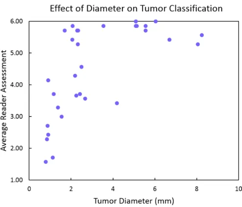
5.4 Averaged reader assessments versus tumor diameters . . . 61
5.5 Examples of control images from the reader study . . . 62
5.6 Examples of tumors from the reader study . . . 63
6.1 ROC Curves of Tortuosity Metrics . . . 69
6.2 Vessel Size vs. Tortuosity . . . 70
6.3 ROC Curve for Multivariate Logistic Regression . . . 72
6.4 Rendered vasculature with tortuosity colormap . . . 74
6.5 Boxplot: DBSCAN Cluster Size . . . 79
6.6 ROC Curve: DBSCAN . . . 80
6.7 Maximum Cluster Size vs Number of Vessels . . . 81
6.8 Maximum Cluster Size vs Tumor Diameter . . . 82
6.9 AUC vs Tumor Diameter . . . 83
6.10 Sensitivity vs Tumor Diameter . . . 84
6.11 ROC curve: clustering analysis of test data . . . 86
6.12 Training data: maximum cluster size vs number of vessels . . . 88
6.13 Training data: maximum cluster size vs tumor diameter . . . 89
6.14 Cluster size vs tumor diameter with fixed intercept regression . . . 90
6.15 Mean tortuosity (SOAM) vs tumor diameter . . . 91
7.1 Beamwidth of 4 MHz transmit pulse . . . 101
7.2 Contrast intensity vs. frame number . . . 104
7.3 In vitro images of targeted microbubbles at 2 pressures. . . 104
7.4 Molecular imaging in vivo . . . 108
7.5 Influence of microbubble size . . . 109
7.6 Comparison of molecular imaging approaches . . . 110
7.7 Comparison of CTR. . . 111
7.8 Comparison of molecular imaging approaches . . . 112
7.9 Overlaid B-mode, molecular, and vascular images. . . 114
7.10 Histograms of distance from targeting and mean vessel size. . . 115
7.12 Overlays of molecular imaging with acoustic angiography. . . 117
7.13 Tortuosity and molecular imaging. . . 123
A.1 Clinical Figure 1 . . . 130
A.2 Clinical Figure 2 . . . 131
A.3 Clinical Figure 3 . . . 132
A.4 Clinical Figure 4 . . . 133
A.5 Clinical Figure 5 . . . 134
LIST OF TABLES
4.1 Tortuosity metrics . . . 39
4.2 Distal tortuosity . . . 46
4.3 Vascular density . . . 49
5.1 ROC regression results . . . 60
6.1 Mean tortuosity and radius . . . 68
6.2 Maximum cluster size . . . 78
6.3 Tumor diameter . . . 85
6.4 Optimal clustering results . . . 87
LIST OF ABBREVIATIONS
2D Two-dimensional
3D Three-dimensional
Ang Angiopoietin
ANOVA Analysis of variance AUC Area under the curve
bFGF Basic fibroblast growth factor
BIRADS Breast imaging reporting and data system B-mode Brightness mode
CEUS Contrast enhanced ultrasound imaging CI Confidence interval
CPS Cadence pulse sequence
CT Computed tomography
CTR Contrast to tissue ratio
dB Decibel
DBSCAN Density based statistical clustering of applications with noise
DM Distance metric
DSPC 1,2-distearoyl-sn-glycero-3-phosphocholine DSPE 1,2-distearoyl-sn-glycero-3-phosphoethanolamine ECM Extracellular matrix
IGF Insulin-like growth factor IHC Immunohistochemical IRB Institutional review board
Hz Hertz
MI Mechanical index
MMP Matric metalloproteinase
MRA Magnetic resonance angiography MRI Magnetic resonance imaging PBS Phosphate-buffered saline PDGF Platelet-derived growth factor PET Positron emission tomography PEG Polyethylene-glycol
PFC Perfluorocarbon
PlGF Placental-derived growth factor PNP Peak negative pressure
Rb Retinoblastoma
Re Reynolds number
RF Radiofrequency
RGD Arg-Gly-Asp
RNA Ribonucleic acid
ROC Receiver operating characteristic ROI Region of interest
SPECT Single photon computed tomography SOAM Sum of angles metric
SV40 Simian virus 40
TNF-α Tumor necrosis factor alpha
ULM Ultrasound localization microscopy VCAM-1 Vascular cell adhesion molecule 1 VEGF Vascular endothelial growth factor
CHAPTER 1
BACKGROUND
1.1 OVERVIEW
This dissertation uses contrast-enhanced superharmonic ultrasound imaging, known as “acoustic angiography”, to examine vascular patterns in tumor and healthy tissue, with a focus on breast cancer. Several aims are addressed in this work:
1. Characterization of normal and pathological patterns of vascularization using acoustic angiography.
2. Determining the performance of acoustic angiography images for tumor detection using visual and quantitative methods.
3. Extension of the high-resolution, superharmonic imaging technique to molecular imaging of targeted microbubbles.
tu-relationship between tumor size and these parameters. Tumor detection, through im-age classification, is performed using qualitative and quantitative approaches and also correlated to tumor size. The development of high-resolution superharmonic molecular imaging is also discussed, and initial experiments were performed to relate molecular and morphological images in tumors.
1.2 BREAST CANCER
Breast cancer represents a significant disease burden in the United States as well as across the world. It is the most common form of cancer in females, accounting for 14% of all new cancer cases in the U.S., and the 3rd leading cause of cancer mortality in females [1]. Approximately 13% of women in the U.S. will be diagnosed with breast cancer during their lifetime. Overall, almost 90% of women diagnosed with breast cancer will survive 5 years after diagnosis, but survival depends greatly on the stage of disease at diagnosis because the relative survival is only 25.9% for metastatic disease, compared to 98.6% and 84.6% for localized and regional disease, respectively [1]. Thus, early detection of tumors before they reach the metastatic stage is an important clinical goal in order to maximize patient survival.
However, mammography is imperfect and results in frequent false positives that pro-duce psychological distress in patients and a high number of biopsies [7–10]. While mammograms are effective at identifying suspicious lesions, they perform poorly at dis-tinguishing between benign and malignant conditions. It is estimated that the cumu-lative risk of a false positive finding after 10 screening mammograms is approximately 50%, which results in several follow-up visits, diagnostic imaging examinations, and sometimes invasive biopsy procedures [11].
While it is unlikely that any imaging modality will soon replace mammography as a widespread screening tool for breast cancer, other imaging modalities are frequently uti-lized for diagnosis of lesions identified by mammography. Due to the high cost and time required for MRI, ultrasound is commonly used for follow-up imaging, but the speci-ficity of both mammography and diagnostic ultrasound is low (approximately 70%), so biopsies are used to confirm diagnosis. This results in a many biopsies performed every year, with a small proportion of them (≈20%) confirming the presence of cancer.
decrease the false-positive rate and could lead to a significant reduction in the number of unnecessary biopsies performed each year.
1.3 TUMORS AND HYPOXIA
Healthy tissue is arranged such that organized layers of cells are supplied with oxygen and nutrients by vasculature in the surrounding stroma. The distribution and spacing of capillaries is largely determined by the metabolic needs of the specific tissue type, with larger spacing in supportive tissues such as smooth muscle and connective tissue and closer spacing in metabolically active tissues such as muscle fibers, and especially the central nervous system [14]. Though distance between capillaries varies between species and tissue types, healthy tissue is usually located less 100 µm from a capillary, and histological examinations by Krough in 1919 observed no tissue beyond 200 µm from an open capillary [15].
Pathological tissue does not display the same regularity seen in healthy tissue, and may exhibit increased, decreased, or heterogeneous vascular spacing, depending on the disease processes occurring. Several studies of the micro-architecture of tumor tissue have shown that while different types of tumors and even adjacent regions of a single tumor are heterogeneous, their growth produces hypoxia, which promotes neovascular-ization through the process of angiogenesis [16–19]. Healthy capillary spacing balances oxygen diffusion with metabolism, because tissue beyond the oxygen diffusion limit will be subjected to hypoxia and metabolic stress, which is common in tumors and contributes to their pathophysiology.
necrosis, but those with a radius less than 160µm did not [16]. Olive et al. measured the oxygen diffusion distance to be 100-200 µm by removing cubes of tumor tissue, incubating them in an oxygenated environment, and then tagging hypoxic cells to mea-sure distance to the oxygen interface [17]. Taken together, these studies suggest that the maximum oxygen diffusion distance in tumors may vary, but that it is unlikely to be greater than 200 µm, and likely less than that in many cases. Hypoxia induces a variety of protective signaling pathways, including anti-apoptotic and pro-angiogenic signal cascades, largely mediated through hypoxia inducible factors, especially HIF-1α (hypoxia inducible factor) [18]. Therefore, as tumors grow larger than the oxygen diffusion limit and become hypoxic, they stimulate angiogenesis to promote vascular-ization of the tumor tissue for the delivery of oxygen and nutrients. Furthermore, even pre-malignant lesions with intact basement membranes can develop necrosis due to in-adequate oxygen supply in an avascular tumor which relies on the diffusion of oxygen and nutrients from the surrounding stroma [19]. Angiogenesis is frequently the obvi-ous result of tumor hypoxia, and the key tumor feature to be used for detection and diagnosis in the imaging experiments described in this work.
1.4 ANGIOGENESIS
be induced by a number of disease processes, including several cytokines which are released by hypoxic tumor tissue.
Angiogenesis, the process of forming new blood vessels from existing ones, is a nec-essary step in wound healing and a component of some healthy physiological processes. However, during tumor formation, the pathways controlling angiogenesis become un-balanced, and a chaotic, disorganized, and dysfunctional network of tumor neovascu-lature is formed. These abnormal tumor vessels do not form hierarchical networks of arterioles, capillaries, and venules, and include locations of transient stasis and flow reversal. Vessel diameters are irregular, often dilated, and do not correlate to blood flow rates. The cellular structure of the endothelial cells, junctions, and associated cells such as pericytes contribute to the vascular dysfunction of tumor neovasculature, which includes leaky and tortuous vessels. [22–25]
Observations of cancer neovascularization go back to at least 1787 when John Hunter, a surgeon, coined the word “angiogenesis”, which was followed by increas-ingly frequent descriptions of abnormal vasculature in tumors during the 19th and early 20th century [26, 27]. It was not until the middle of the 20th century that can-cer angiogenesis was first recognized as a vital step for tumor growth when several researchers proposed and tested the hypothesis that tumor-derived factors served to stimulate neovascularization for tumor growth [28–31].
molecular pathways appears to be disturbed by tumor growth, and angiogenesis is fur-ther stimulated by hypoxia induced by insufficient vascular supply of the dsyfunctional neovasculature, thus forming a positive feedback cycle [33, 34].
Sprouting is often regarded as the primary mechanism of angiogenesis. It involves the creation of a new vessel through rearrangement and proliferation of endothelial cells into stalk and tip cells. The tip and stalk cells emerge from an existing vessel into surrounding stroma and tissue in response to soluble molecular signals and chemical gradients, and sprouting terminates through anastomosis of two nearby sprouts, result-ing in lumenization of the nascent vessel [35]. Intussusception is another mechanism of angiogenesis distinct from sprouting [36]. Intussusceptive angiogenesis involves the formation of transvascular pillars within the lumen of an existing vessel to split it into two lumens [37].
One of the molecules strongly related to the process of angiogenesis is vascular endothelial growth factor, or VEGF. VEGF-A was also called vascular permeability factor when it was discovered, due to its propensity to produce vascular leakage [38]. VEGF-A promotes angiogenesis by guiding sprouts, inducing proliferation in the stalk cells and directing filopodia and migration across the concentration gradient in the tip cells [39]. Signaling of angiogenesis by VEGF is primarily through the vascular endothelial growth factor receptor 2 (VEGFR2) tyrosine kinase [40].
down basement membrane and extracellular matrix in order to make room for sprout invasion, while Ang1 promotes vessel maturation [44]. Breakdown of the extracellu-lar matrix can cleave several growth factors harbored in the matrix, which are then released into the interstitium, further enhancing angiogenesis. Matrix-bound growth factors include basic fibroblast growth factor (bFGF), VEGF, and insulin-like growth factor-1 (IGF-1) [35]. Placental derived growth factor (PlGF) can also contribute to angiogenesis, possibly through the recruitment of bone marrow derived endothelial pro-genitor cells, and due to synergistic effects with VEGF as both growth factors bind to VEGFR1, a decoy receptor for VEGFR2 [45].
Decades of research have led to the production of anti-angiogenic drugs, primarily through inhibition of vascular endothelial growth factor (VEGF) and one of its recep-tors, VEGFR2. However these drugs that aim to inhibit angiogenesis have been largely ineffectual, and the modest improvements in survival in a few types of cancer (such as metastatic colon cancer) do not extend survival more than a few months [46, 47]. It is clear from these clinical experiences and the disconnect between patient outcomes and pre-clinical studies in implanted tumor models that we do not fully understand the complex process of angiogenesis. Though researchers are unable to successfully control tumor angiogenesis, its pervasiveness makes it an attractive target for imaging. Furthermore, we hypothesize that the morphological abnormalities common to tumor neovasculature can be observed using acoustic angiography, thus painting a picture of microvascular structure and enabling vascular tortuosity to be quantified and utilized as an imaging biomarker.
1.5 WHY IS TUMOR VASCULATURE TORTUOUS?
vessels. In tumour vessels, tortuosity is believed to be a hallmark of defective structural properties.” [48]. The underlying mechanism of vessel tortuosity has not been traced to a single cause, but seems instead to be related to a number of molecular and physical conditions in the tumor micro-environment. As discussed in the previous section, tumor angiogenesis is abnormal and produces disorganized and dysfunctional vasculature [49]. Structurally, tumor vessels (especially venules and veins) are dilated and tortuous, and arteriovenous anastomoses are common, resulting in abnormal flow, including transient stasis and flow reversal [23].
been attributed to a restriction on lengthening, which is imposed by vessel anchoring at fixed points upstream and downstream. As a result, growing tumour vessels cannot extend linearly and so they coil.” [56]. Hartnett et al. also attribute tortuosity to lengthening, though not specifically attributable to VEGF-A: “tortuosity is believed to be a form of angiogenesis through vessel lengthening” [54]. However, VEGF-C was also found to influence tortuosity because VEGF-C over-expressing tumors demonstrated a dose-dependent response in venous dilation and tortuosity [57]. Furthermore, metabolic stress (hypoxia, low pH, hypoglycemia) generated by the tumor and the immune and inflammatory response (mediated by monocytes, macrophages, platelets, mast cells, and leukocytes) can trigger angiogenesis, resulting in tortuosity, through many of the molecular pathways already mentioned [42].
In addition to the molecular factors that influence vessel morphology, the physical presence of the tumor itself may contribute to vascular tortuosity by displacement of existing vessels by the expanding tumor mass. Solid stress produced by the prolifer-ating tumor and the extracellular matrix can produce forces strong enough to cause transient vessel collapse or stenosis [58]. Stenosis itself has also been observed to pro-mote distal tortuosity, which is likely be caused by flow disturbances [59]. Also, leaky tumor vasculature allows plasma extravasation, which coupled with the lack of func-tional lymphatics, results in elevated interstitial pressure and altered trans-vascular flow patterns [60].
disturbances proximal and distal to the locations of curvature and observed that flow disturbances were related to curved, tortuous segments [61].
In fluid dynamics, the Reynolds number (Re) is a dimensionless parameter that describes the ratio of inertial to viscous forces of fluid flow. Flow is considered laminar for Reynolds numbers below 2000 for steady flow in a straight tube, but Stehbens et al. observed flow disturbances at much lower Re in tortuous tubes [61]. The most highly tortuous tubes produced flow disturbances including secondary (helical) flow, backflow, and vortex shedding at the lowest Re. In animal studies with tortuous U-shaped vessels created by microvascular surgery, tears in the intima were observed [62] and endothelial damage was seen in areas of high curvature, whereas proliferative lesions were seen in locations of lower curvature [63]. Thus, tortuosity itself could produce a positive feedback loop by producing flow disturbances that alter endothelial growth and death differentially in adjacent segments of a vessel. Additionally, stenosis produced by increased mechanical stress from the tumor and ECM could also create flow disturbances and trigger a non-uniform endothelial response that could result in tortuous vessel growth. Finally, thrombosis has also been observed in tortuous vessel segments and in shear flow conditions, and thrombosis can induce capillary growth through molecular angiogenic signaling pathways [41].
studies, VEGF RNA is also overespressed in infants with tortuous retinal vascula-ture [68]. Additionally, neutralizing VEGF has been seen to reduce retinal tortuosity in a rat model of retinopathy [54], further implicating the strong association between VEGF and vascular tortuosity in the retina, independently of any correlations found between tortuosity and increased blood pressure.
Furthermore, the possible association between hypertension and tortuosity is un-likely to extend to tumors for several reasons. First, the arterial pressure in tumors is approximately equal to that of normal tissue, whereas the venous pressure is signifi-cantly lower [23]. Thus the average blood pressure in tumors is decreased rather than increased, which should correlate with reduced tortuosity according to retinal models. Second, the material properties and microenvironment of a tumor are different from the latex tubing models [66], numerical models [69] and the retina itself. Tumors and the associated stromal cells often produce a stiffer lesion, largely due to abnormal growth and function of the extracellular matrix [70]. These factors would tend to reduce the vascular displacement (and therefore tortuosity) induced by elevated blood pressure.
1.5.1 OBSERVATIONS OF TORTUOSITY IN DISEASE
1 diabetes patients [73]. Retinal tortuosity has also been correlated to cardiovascular disease [51, 74] and anemia [75].
Tortuosity has also been described using other imaging modalities outside of the retina. Subjective ratings of tortuosity in angiograms of intercostal arteries showed a trend of increasing tortuosity with age [76]. Subjective tortuosity assessment was also used to analyze 2-D and 3-D CT angiography, MRI, and X-ray images of head and neck vasculature in patients with Loeys-Dietz Syndrome Type 1 [77]. MRI an-giography imaging of connective tissue disorders also revealed tortuosity in thoracic vertebral arteries [78]. Tortuosity of major cerebral vessels, particularly those in the neck, was found in 25% of patients with symptoms of cerebrovascular disease [59]. The authors attributed the tortuosity they observed to hypertension and arteriosclero-sis. 3-D imaging in the aorta and iliac arteries was used to correlate tortuosity (both subjective ratings and computerized quantifications) to outcomes of aneurysm repair procedures [79]. Measurements of tortuosity based on calculations of curvature were derived from 3-D MRI imaging in order to model blood flow patterns in the femoral artery to predict probable locations of atherosclerosis and to explain differences in the prevalence of atherosclerosis in the superficial femoral artery in men and women [80]. Bullitt et al. observed that a healthy aging population exhibited few changes in vas-cular tortuosity, but that fewer resolvable vessels were visible in oder adults [81]. She and colleagues also compared cerebral tortuosity of aged individuals with varying levels of physical activity, and found that aerobic activity was correlated to lower tortuosity and higher numbers of small vessels in the brain [82].
work. Ultrasound imaging has also been used to observe tortuous vasculature in tu-mors, though not as extensively as tortuosity has been studied in the retina using optical fundus imaging. Tortuosity observed in 3-D power Doppler ultrasound was indicative of ovarian malignancy [85], and microbubble-enhanced color Doppler ultrasound made tortuous vasculature more apparent in tumors [86].
1.5.2 MEASURING TORTUOSITY
Tortuosity, a quality describing the degree of bending and twisting exhibited by a vessel, has been used to describe retinal fundus images, Doppler ultrasound, x-ray angiography, and in cerebral magnetic resonance angiography (MRA), as described in the preceding sections [13, 65, 85–90]. Early evaluations of tortuosity were subjective, visual assessments of the degree of abnormality observed in the images [75, 76, 86, 91]. Eventually, quantitative metrics describing tortuosity based on vessel length, local cur-vature, and locations of inflection were derived, and with the increasing prevalence of 3-D medical imaging data, 2-D tortuosity metrics were extended to 3-D [78–80, 87, 92]. However, despite the interpretive value of images displaying vascular morphology and the increasing variety of metrics describing tortuosity, few clinical standards exist for evaluating abnormal tortuosity and making diagnoses. Retinal imaging has often re-sulted in subjective classifications of tortuosity, or simple metrics such as the ratio of vessel length to distance between endpoints. However, Sodi et al. incorporated mea-surements of local curvature of the 2-D vessels including sums or products of curvature along the vessels and another, the ”triangular index”, based on fitting triangles [87]. Others have used curvature based metrics including sum of squared curvature along the vessel path [50].
sensitive to morphological changes induced by cancer angiogenesis, as imaged by ultra-sound acoustic angiography. Additionally, metrics will be combined into a multivariate model for prediction of malignancy based on the combined tortuosity of an acoustic angiography image. Cancer detection using the abnormal vascular “fingerprint” of a tumor is a novel imaging biomarker and may enable the detection of smaller lesions than currently possible. This project aims to develop estimates of the sensitivity and specificity for the detection of tumors smaller than 1 mm3 in diameter as a step forward in the goal of early detection and improving the specificity of diagnosis
1.5.3 METRICS DEFINED
The two tortuosity metrics used throughout this work are the distance metric and the sum of angles metric. Both metrics are computed using the centerline of the vessel and do not take local vessel diameter into account. While both metrics are length invariant, consistent voxel sizing and sampling should be maintained to ensure accurate comparisons between images.
DISTANCE METRIC
The distance metric is the most commonly cited measure of general “tortuosity” in both 2-D and 3-D imaging, and simple to calculate at any scale. The distance metric is the ratio of the total path length of the vessel to the Euclidean distance between the vessel endpoints. Thus, a straight vessel has a distance metric value of 1 and increases for curved vessels as total path length increases relative to distance between endpoints. For a point,P, along the centerline of a vessel, the distance metric is defined as follows:
DM =
n−1
P x=1
kPx−Px+1k
kPx−Pnk
The distance metric is a unitless quantity since it is the ratio of two distances.
SUM OF ANGLES METRIC
The sum of angles metric, on the other hand, is computed by calculating the an-gle between successive trios of points along the vessel and summing them, followed by normalizing the sum of the angles by the path length of the vessel to ensure length invariance. Length invariance is preferred so that tortuosity values are not dependent on the number of points per vessel, and vessel length can be included as an additional metric in multivariate analysis if it provides useful information for discrimination be-tween tumor and control vasculature. The angles along the centerline are computed by taking the inverse cosine of the dot product between the two unit-length vectors formed by 3 points, as follows:
SOAM =
n−3
P x=1
arccoskV1V1k · V2
kV2k
n−1
P x=1
kPx−Px+1k
(1.2)
Vectors V1 and V2 are the vectors between subsequent points along the centerline.
Thus, (V1 = Px+1 −Px) and (V2 = Px+2−Px+1) for n points (P) along each vessel.
The sum of angles metric has units in radians per unit length.
CHAPTER 2
CONTRAST ENHANCED ULTRASOUND IMAGING
2.1 MICROBUBBLE DEVELOPMENT
Contrast enhanced ultrasound imaging began with the development of microbubbles to enhance signals from the circulatory system in order to overcome the weak scattering by blood. Dr. Charles Joiner, a cardiologist, noticed brief ultrasound enhancement while injecting indocyanine through a catheter in the left ventricle, and it was later discovered that the source of the echoes were bubbles on the catheter tip [93]. Prior to the formulation of encapsulated microbubbles, indocyanine green and agitated saline along with other agents were used in echocardiography, often to detect shunts since the free gas bubbles were removed from circulation very quickly (after a single pass through the lungs) [94–99].
The discovery that contrast could be improved by mixing blood with the saline prior to agitation led to the development of Albunex (Molecular Biosystems, San Diego, CA), a microbubble with an air core stabilized by shell composed of human serum albumin [100,101]. Echovist (Schering AG, Berlin, Germany) was a first generation microbubble stabilized with D-galactose, but these bubbles still did not persist in circulation [93]. The agent Levovist was a successor of Echovist, and it incorporated palmitic acid to act as a surfactant to improve the longevity of the agent [93].
to cores of high molecular weight gases to slow diffusion of the gas through the mi-crobubble shell. Polyethlyene glycol (PEG) was incorporated to prolong circulation time, minimize coalescence, and improve solubility [93]. Optison (Molecular Biosys-tems, San Diego, CA, currently GE Healthcare Bio-sciences, Pittsburgh, PA) contains a perfluorocarbon (PFC) core with an albumin shell, and reported stronger harmonics than Albunex, the previous albumin-encapsulated microbubble [98]. Sonovue (Bracco, Milan, Italy) consists of a phospholipid shell and a sulfur hexafluoride core, while Defin-ity (Lantheus Medical Imaging, N. Billerica, MA) pairs a phospholipid shell with a PFC core [93]. Currently, the FDA approves of Optison and Definity for echocardiography, specifically opacification of the left ventricle. Sonovue, now known as Lumason in the United States, is approved for liver imaging in adults and children as of 2016.
2.2 MICROBUBBLE PROPERTIES
Microbubbles are blood-pool agents, confined to the circulation due to their size of approximately 1-7µm. The shell material is thin in comparison to the microbubble size, with thickness between 10 and 200 nm [102]. Microbubbles are cleared primarily by the reticulo-endothelial system, with microbubbles retained in the liver and spleen by phagocytic cells (macrophages and specialized Kupffer cells) [103]. The core gases that diffuse into circulation are cleared by the lungs, and human pharmacokinetic studies showed that the expired half-life of sulfur hexafluoride and PFC gases was very quick, on the order of few minutes, and there was little to no detectable gas in any patients after 90-120 minutes [104, 105].
mismatch with surrounding blood and tissue due to the low density and very high com-pressibility of the gas core. The physical properties of microbubbles enable them to very effectively reflect ultrasound, leading to enhancement in B-mode images, but it is their compressibility that leads to unique non-linear properties that differ greatly from tis-sue [106]. At very low pressures, the microbubble diameter oscillates with the positive and negative cycles of the transmitted ultrasound wave. At more moderate pressures, such as 150-300 kPa (in vivo), microbubble expansion increases relative to the contrac-tion, and the speed of the contractive cycle is faster than the expansive cycle, leading to the production of non-linear echoes. Higher pressures result in asymmetric expansion and microbubble fragmentation, but it is worth noting that the precise thresholds de-termining microbubble behavior vary with diameter and shell composition, ultrasound frequency and pulse repetition rate, as well as boundary conditions. However, the harmonics (integer multiples of the fundamental frequency), subharmonics (half the fundamental frequency), ultraharmonics (half-integer multiples of the fundamental), and superharmonics (combined higher harmonics, ultraharmonics, and non-integer fre-quency response) originating from microbubbles are distinct from the behavior of tissue, and thus are used to separate microbubble signals from the surrounding tissues.
2.3 CONTRAST IMAGING TECHNIQUES
specificity and the contrast-to-tissue ration (CTR) was not high. Therefore, contrast pulse sequences known as pulse inversion and amplitude modulation were developed to take advantage of microbubble nonlinearity that was not restricted to the second har-monic signal [111–115]. Subharhar-monic imaging (at half the frequency of the transmitted pulse) is also more specific to microbubble contrast, but tends to lack the resolution of some of the multi-pulse techniques due to the low frequencies used [116, 117]. Several encoded imaging methods have also been tailored for contrast imaging, including chirp and Golay encoding [118–121]. In recent years, ultra-fast plane wave imaging has also been extended to contrast imaging using both contrast-specific pulse schemes as well as contrast-enhanced Doppler [122, 123].
More recently, ultrasound localization microscopy, otherwise known as super res-olution, has been developed to provide very high resolution vascular images. These techniques were inspired by microscopy methods which rely on the stochastic blinking of fluorophores to separate their signals and improve resolution beyond the diffraction limit [124, 125]. The first description of a similar implementation in ultrasound was by Viessmann et al. using low concentrations of contrast to detect and localize single bubbles in tubes, accumulating a sufficient number of frames to combine into an im-age over a long period of time [126]. This was closely followed by another group who imaged single bubbles in phantoms encased a human skull [127]. Desailly et al. then used microfluidic channels to measure resolution, and incorporated ultrafast imaging to avoid diluting contrast and acquire data more quickly, but their work was limited
toin vitro experiments [128]. Later, Christensen-Jeffries et al. used the dilute, “single
a year later, Errico et al. demonstrated the first super-resolution images using ultra-fast acquisition in vivo, imaging the brains of rats [130]. This year, Lin et al. applied the ultra-fast super resolution technique to image tumor vasculature, also in rats, and combining several 2D slices into a 3D projection [131].
The main disadvantages of ultrasound localization microscopy or super-resolution imaging are the long acquistions times, even with ultra-fast imaging, and computa-tionally intense image reconstruction. Errico et al. were able to acquire almost 75,000 frames to reconstruct an image of the cortex of a rat (3.5 mm in dept depth) in 2.5 minutes, while a larger image to 11.6 mm required 10 minutes. The long imaging times make physiologic motion a problem and therefore the French group focuses their imag-ing on the brain because the tissue is extremely stationary when the skull is held in place with a sterotactic device [130]. Lin et al. was able to acquire a sufficient number of images for a 2D image in 26 seconds, but the total acquistion time of 3D images with 200 µm slice spacing was over 30 minutes [131].
2.4 SUPERHARMONIC IMAGING
2.4.1 IMPLEMENTATION
bandwidth) elements alternating with 2.8 MHz (80% bandwidth) elements. The very low frequency transmit (below 1 MHz) was selected to minimize nonlinear propagation through tissue, a frequency dependent phenomenon [133, 134], and because their de-sired application is detection of myocardial perfusion. They transmitted an 800 kHz pulse with the low frequency elements and received with the high frequency elements, and results included anin vitro image of microbubbles in a tube and a figure reporting CTR in dB for the received RF data at different frequencies which showed a peak CTR receiving the superharmonic signals at 3 MHz. They then followed this conference pro-ceeding with 2 full length manuscripts describing the transducer and superharmonic imaging experiments [135, 136]. In these works, they compared transmitting at 0.8 and at 1.7 MHz. They found that the maximum CTR was approximately 30 dB at the 4th and 5th harmonic levels when transmitting at 1.7 MHz, and as high as 80 dB (also at the 4th and 5th harmonics) when transmitting at 0.8 MHz. They attributed the gain in CTR to reduced frequency-dependent nonlinear propagation at lower transmit frequency. They also demonstrated thein vivo feasibility by imaging the heart of a pig, transmitting at 0.8 MHZ with a MI of 0.4 and receiving with the 2.8 MHz transducer and using a bandpass filter of 2.7-4.7 MHz. Further work described their interleaved transducer design in more detail and demonstrated imaging of myocardial perfusion in a pig model [137, 138].
microbubbles [140]. Later, they developed a dual frequency array design with a 5.4 MHz linear array flanked by two 1.5 MHz arrays, which was used forin vitro [141] andin vivo
experiments [142] showing improved resolution with superharmonic contrast detection and demonstrating slow-time filtering methods for separating signal from adherent and flowing microbubbles. The animal model used was FVB mice with Met-1 breast tumors implanted in the mammary pads, a model chosen for it’s known phenotype of significant angiogenesis.
2.4.2 MICROBUBBLE PRODUCTION OF SUPERHARMONICS
Though non-linear propagation of ultrasound through tissue occurs to some extent, the production of superharmonics is microbubble specific phenomenon. While very low pressure imaging schemes are frequently used in contrast specific pulse sequences (such as pulse inversion and amplitude modulation) in order to minimize tissue artifacts and microbubble destruction, the production of superharmonics requires somewhat higher (moderate) pressures. Kruse and Ferrara attribute the production of wideband super-harmonics to “high bubble wall velocity and acceleration achieved when a microbubble collapses”, a theory supported by bubble modeling using the Rayleigh-Plesset equation, or to the alternate theory that shell rupture releases free gas into the fluid, resulting in “stronger oscillation of a free gas bubble compared to the damped oscillation of an en-capsulated bubble” [139]. They reported that for 10 cycle pulses, pressures of 100-200 kPa were necessary to induce the production of wideband, superharmonic, transient echoes, and that higher harmonic content increased with increasing pressure. Trans-mitting at 0.8 MHz, Bouakaz imaged myocardial contrast at MI close to 0.4 inin vivo
Lindsey et al. performed detailed experiments in order to understand the relation-ships between frequency (both transmitted and received), pressure, and microbubble diameter on the resulting images, specifically the CTR and resolution. He found that the resolution is primarily dictated by the receiving frequency, thus high frequency receiving transducers should be selected for imaging microvascular morphology. As reported in previous studies, the transmitted pressure influenced CTR, with CTR in-creasing with pressure until a threshold was reached, though the specific pressure at which this occurs varies with other factors such as frequency, microbubble attributes,
andin vitro versusin vivo conditions [159]. In a subsequent publication, they reported
that production of superharmonics does not rely on complete microbubble destruction, but can also be produced by gradual dissolution of a microbubble over several pulses. However the magnitude of the superharmonic signals produced by gradual dissolution (microbubble shrinking) is much weaker than that produced by microbubble destruc-tion.
CHAPTER 3
MATERIALS AND METHODS
3.1 ANIMAL MODELS
The majority of this project utilized a genetically engineered mouse model of breast cancer. The tumor-bearing animals were female C3(1)/Tag mice, which develop tumors spontaneously in the mammary pads. C3(1)/Tag mice are a model of basal breasts cancer in which oncogenesis is driven by the inactivation of the p53 and retinoblastoma (Rb) oncogenes by the siminan virus 40 (SV40) large T-antigen [161, 162]. Mammary carcinomas develop by 16 weeks, with abnormal ductal hyperplasia occuring earlier, mimicking the progression of breast cancer in humans. Female FVB/NJ littermates not carrying the transgene served as controls. Mice were bred and obtained from the Mouse Phase 1 Unit at the University of North Carolina at Chapel Hill, which is supported in part by the University Cancer Research Fund. For imaging, mice were anesthetized with 1-2% aerosolized isoflurane in oxygen for imaging, and hair on the ventral side was removed with clippers followed by chemical depilation to allow visualization of the caudal mammary pads. With assistance of the Animal Studies Core, a 27 gauge catheter was placed in a tail vein for injection of the contrast agent. The Animal Studies Core is supported in part by an NCI Center Core Support Grant to the UNC Lineberger Comprehensive Cancer Center.
fresh tissue while animals were anesthetized. Tumor material was obtained from the Dewhirst laboratory at Duke University, Durham, NC, who received their tumor tissue from the Bull laboratory at the Univeristy of Texas M.D. Anderson Cancer Center, Houston, TX. They remark that the tumor was “originally isolated from the subcutis of rats that were given the carcinogen methylcholanthrene and was maintained by serial transplantation” [163, 164]. Anesthesia was induced with 5% aerosolized isoflurane in oxygen and reduced to approximately 2% during imaging. The imaging region was depilated with clippers and chemical depilation, and a 24 gauge catheter in the tail vein provided vascular access for contrast agent injection.
Animals were supported by a heated stage to maintain body temperature during all imaging studies, and ultrasound gel was used to couple the transducer to the skin surface. All studies involving animals were reviewed and approved by the Institutional Animal Care and Use Committee at the University of North Carolina at Chapel Hill.
3.2 MICROBUBBLE CONTRAST AGENTS
a rate of 30µL per minute using a syringe pump (Harvard Apparatus, Holliston, MA) during contrast-mode in vivo imaging.
3.3 IMAGE ACQUISITION
B-mode and dual-frequency images were acquired with a VisualSonics Vevo 770 sys-tem (FUJIFILM VisualSonics, Toronto, ON, Canada) using a modified RMV707 (30 MHz center frequency) or RMV710 (25 MHz center frequency) transducer. A 4 MHz an-nular element was added confocal to the high frequency element, with the focus at 12.7 mm (RMV707) or 15 mm (RMV710), as shown in figure 3.1. For dual-frequency super-harmonic imaging, the high frequency element was disabled, and the trigger from the Vevo 770 scanner was synchronized with an arbitrary waveform generator (AFG3101 or AWG2021, Tektronix, Beaverton, OR) used to produce a single-cycle, windowed, sinusoidal waveform which was then amplified (ENI, Rochester, NY) before exciting the low frequency element [147]. Transducer output was calibrated using a needle hy-drophone (HNA400, Onda, Sunnvale, CA), acquisition board (Signtec PDA14, Corona, CA), and motion stage (Newport XPS, Irvine CA) programmed in LabView (National Instruments, Austin, TX).
step size of 100 m and a frame rate of 4 frames per second, unless otherwise specified. In dual-frequency contrast mode, frame smoothing was used to average 2 acquisitions together to form each frame. The field of view was 2.5 by 2.5 cm in the axial and lateral dimensions, and determined by the user in the elevational direction.
Figure 3.1: This photograph shows the center high frequency element (25 MHz) sur-rounded by the low frequency annular element (4MHz). Both elements have curved lenses to focus them to a depth of 15 mm.
3.4 IMAGE PROCESSING
developed tumors over the course of the study. B-mode measurements were selected for determining tumor dimensions instead of caliper measurements due to the higher precision. Caliper measurements tended to vary by as much as a millimeter or more, possibly due to different amounts of tissue compression. Measurements from B-mode images depended on image quality and definition of the boundary based on image echogenicity, but were superior to physical measurements made with calipers.
6.
The distance metric is a ratio of the path length of a vessel to the Euclidean distance between vessel endpoints, and is one of the most common quantifications of “tortuosity” in the literature. The sum of angles metric is calculated by taking the sum of the angle (in radians) between 3 points along the centerline of the vessel and normalizing by path length (in mm). Thus the units of the sum of angles metric are radians per unit distance. The distance metric, on the other hand, is a dimensionless quantity that is the ratio of two lengths. For analysis of specific regions of images, such as tumors, regions of interest were segmented manually by interactively drawing polygons (using roipoly in Matlab) on individual slices of the grayscale ultrasound images and concatenating the 2D regions into a 3D segmented volume or ROI. See chapter 1, section 1.5.2 for more detailed discussion and definition of the tortuosity metrics.
3.5 STATISTICAL ANALYSIS
CHAPTER 4
CHARACTERIZING VASCULATURE IN TUMOR REGIONS
4.1 OVERVIEW
As discussed in chapter 1, tumors are known to produce abnormal vascular struc-tures. Therefore, an imaging technique which is capable of resolving vasculature with clarity could provide useful information about tissue for characterization, detection, and diagnosis of tumors. The current ultrasound acoustic angiography technology is capable of producing high-contrast images of vasculature as small as 100-150 µm in diameter, to a depth of approximately 2 cm. This can be accomplished safely, as ul-trasound does not expose the subject to any ionizing radiation and clinically approved contrast agents have a strong safety profile. This chapter is devoted to characterizing differences between tumor and normal vascular patterns that are detectable in acoustic angiography images. We will explore how tortuosity and vascular density compare in regions of tumor and healthy vasculature, as well as analyzing how the vasculature in tissue surrounding a tumor is affected by the presence of the tumor.
since soft tissue sarcomas are heterogeneous and represent less than 1% of malignan-cies in the United States [173]. Therefore, the majority of the experiments in this work utilized a spontaneous mouse model of breast cancer, the C3(1)/Tag.
The benefit of a model in which tumors develop spontaneously (in this case driven by the inactivation of the p53 and Rb tumor suppressor genes) is that any tortuosity observed can be attributed to the tumor development process and not a wound heal-ing response due to tumor implantation, which was one of the limitations of earlier studies. Additionally, the progression of mammary carcinomas that develop in female C3(1)/Tag mice is very similar to the stages observed in human breast neoplasms [162], making it an excellent model for the characterization of early-stage lesions. Finally, the mouse model of basal breast cancer is clinically significant because breast cancer has widespread incidence and the hormone receptor negative tumor types do not have targeted therapies and suffer from a worse prognosis. Additionally, breast cancer rep-resents a tumor type that is somewhat superficial, which may enable the translation of acoustic angiography imaging to the clinic. Ultrasound already plays an important role in the diagnosis of breast lesions, making the development of technologies with improved diagnostic information extremely relevant.
This chapter examines the vascular morphology of tumors by using regions of inter-est (ROIs) to isolate tumor vasculature for comparison with normal vessels. ROIs are then expanded to explore the tortuosity of vasculature in tissue immediately surround-ing a tumor. The hypotheses addressed in this chapter are:
1. Tumor vasculature is significantly more tortuous than that of normal, healthy tissue.
2. The density of vasculature within tumors is higher than in surrounding tissues.
tumors to approach the values seen in normal tissue.
Figure 4.1 illustrates the difference between conventional B-mode imaging at a single center frequency, and the dual frequency contrast imaging technique, acoustic angiog-raphy.
Figure 4.1: Conventional B-mode image (25 MHz) reconstructed in the coronal plane from images acquired 100 µm apart axially and the co-registered maximum intensity projection of the dual frequency vascular image acquired during microbubble infusion by transmitting at 4 MHz and receiving at 25 MHz.
linear or smoothly curved. The tumor images (bottom row) show tortuosity in the vessels supplying and penetrating the tumors. The middle tumor has clearly higher vascular density that the surrounding tissue, evident by the bright contrast signal in the tumor region coming from both resolvable and sub-resolution vasculature.
4.2 TORTUOSITY ANALYSIS
The tortuosity metrics used in this chapter are the distance metric and sum of angles metric, computed using Bullitt’s algorithm, and described in sections 1.5.2 and 3.4. The distance metric is the ratio of path length to distance between endpoints of a vessel and the sum of angles metric is the sum of the angles between points along the centerline and normalized by path length. The distance metric effectively captures the tortuosity of arching vessels with low spatial frequency and high amplitude oscillations, whereas the sum of angles is more sensitive to curves that vary at a high spatial frequency, but a low amplitude. Such curves appear sinusoidal or spiraling, and the local curvature along the vessel can be high without increasing the overall length of the vessel substantially. Both types of tortuosity are seen in tumor vasculature, and chapter 6 will discuss them in combination, but this chapter examines each metric independently by comparing vessels contained within tumor regions to healthy abdominal vasculature in control mice.
4.2.1 TUMOR REGIONS OF INTEREST
Vessels from the tumor ROIs and control images were pooled, and a two-sided t-test was used to test for a difference in means for each metric. Pooling vessels from every image together resulted in a total of 1,556 control vessels and 746 tumor vessels. The lower number of tumor vessels is due to the smaller total volume analyzed because tumor images were masked to include the tumor ROIs and exclude surrounding tissue in this analysis. The mean and standard deviation of the DM was 1.255 ± 0.371 for controls versus 1.431 ± 0.596 for the tumor ROIs, with p<0.01 for the difference between groups. The SOAM exhibited an even larger difference in means with control images having a mean value of 22.51 ± 9.45 versus 35.92 ± 13.49 for the tumor ROIs (p<0.01).
As an alternative to pooling the vessels from all images together, we can take the mean value of a tortuosity metric for each image or ROI, and use this mean values to represent an volume. With a single value per metric for each image or ROI, we can visualize the separation between tumors and controls. Figure 4.3 is a scatter plot of data points representing each tumor ROI or control image, with the 2 tortuosity metrics (SOAM than the DM) as the axes. This plot represents control data points with orange squares and tumor data points with blue diamonds in order to visually assess their separation. We can notice that there is some separation along the horizontal axis, representing the distance metric, but that there is much more separation between the two groups along the vertical axis, representing the sum of angles metric. This plot reveals that the magnitude of difference and class separation between tumor ROIs and controls is superior for the sum of angles metric than for the distance metric.
Figure 4.3: Mean distance metric and mean sum of angles metric for 24 tumor ROIs and 20 control images.
Table 4.1: Mean and standard deviation of means for the distance metric and sum of angles metric.
DM SOAM
Tumors 1.43 ±0.11 35.68 ± 4.85 Controls 1.28 ± 0.072 21.64 ± 2.75
metric and p= 1.7×10⁻¹⁴ for the sum of angles metric. In order to compare the value
of the sum of angles metric and distance metric for their power to discriminate between the tumor and control classes, we can plot receive operator characteristic (ROC) curves and compare the area under the curve (AUC) in figure 4.4.
Figure 4.4: ROC curves for the distance metric (left, in green) and the sum of angles metric (right, in blue) using the mean value of each image for classification.
4.2.2 TORTUOSITY AND TUMOR SIZE
Though images of tumors of different sizes visually reveal that more tortuous ves-sels are apparent in larger tumors compared to smaller tumors (see figure 4.2), linear regression resulted in weak correlation with tumor size for both the DM and SOAM, with only the DM resulting in a statistically significant trend (R2 = 0.26, p = 0.01),
shown in figure 4.5. Linear regression between tumor diameter and the sum of angles metric resulted inR2 = 0.07 and p= 0.19.
Figure 4.5: Scatterplot of the mean DM and SOAM tortuosity of 24 tumors versus the maximum tumor diameter in millimeters. The distance metric is indicated with blue circles, and the sum of angles metric is indicated with green triangles.
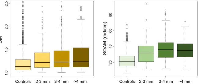
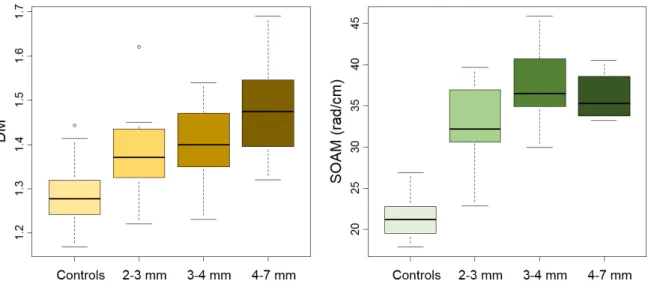
mm, and 4-7mm in diameter. Boxplots of tortuosity for the controls and the 3 tumor size classes show a trend of tortuosity increasing slightly with tumor size, despite poor correlation using linear regression in figure 4.5. Figure 4.6 shows the results for diameter subsets of pooled vessels and figure 4.7 shows the same data using image means instead of pooled vessels.
Figure 4.6: Boxplots of controls and 3 size classes of tumors showing differences in pooled vessel statistics for the distance metric (left) and sum of angles metric (right). Adapted and reprinted from Ultrasound in Medicine & Biology, Volume 41, Issue 7, Sarah E. Shelton, Yueh Z. Lee, Mike Lee, Emmanuel Cherin, F. Stuart Foster, Stephen R. Aylward, Paul A. Dayton, Quantification of Microvascular Tortuosity during Tumor Evolution Using Acoustic Angiography, Pages 1896-1904, c2015, with permission from Elsevier.
Figure 4.7: Boxplots of controls and 3 size classes of tumors showing differences in statistics of image means for the distance metric (left) and sum of angles metric (right).
vessel statistics, and the p value of the image mean statistics was low (p = 0.07) but not significant.
4.2.3 TORTUOSITY BEYOND THE TUMOR MARGIN
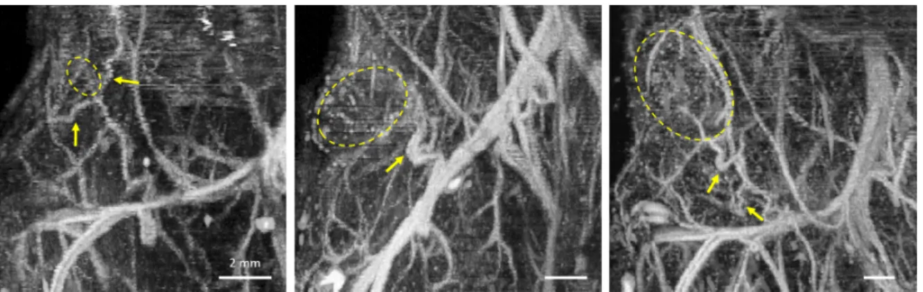
Acoustic angiography images and the analysis in the previous section have shown that blood vessels within a tumor are more tortuous than normal vasculature, but some images also show tortuous vessels outside of tumors, but they tend to be nearby and often connecting the tumor vasculature to other vascular beds. Figure 4.8 shows examples of 3 tumors with clearly tortuous vessels outside the tumor margin. This observation leads to the question of whether vascular tortuosity outside a tumor is related to proximity to the boundary.
Figure 4.8: These maximum intensity projections in the coronal plane illustrate three tumors with tortuous vasculature outside of the tumor margin. The tumor locations are roughly indicated by the dashed yellow lines and the tortuous vessels that can be seen supplying these tumors are indicated by the yellow arrows. Scale bars represent 2 mm.
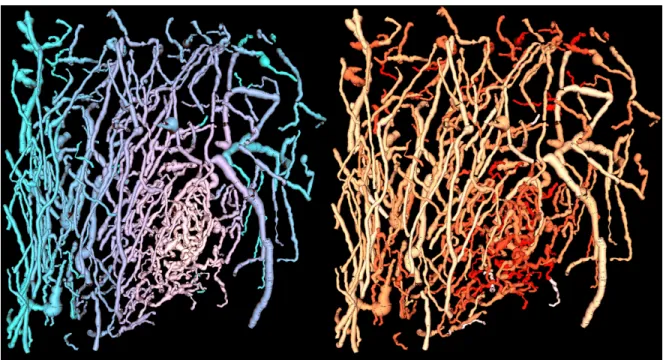
ROI evolution and vessel segmentation. Each dilation of the ROI increased the radius by 2 mm, but the ROIs were not required to be spherical, so the “radius” of dilation is approximate and determined by morphological dilation on the binary ROI mask.
Figure 4.9: Renderings of vasculature within and surrounding a small tumor. The smallest ROI in the first panel contains the tumor and a margin of 2 mm. Then, from left to right each panel shows the result as the mask was successively enlarged by 2 mm, incorporating more of the surrounding vasculature with each subsequent dilation.
The smallest ROI in figure 4.9 contains the tumor vasculature and vessels from a margin of 2 mm around the tumor. The mean tortuosity of each ROI was regressed against distance from the tumor margin using least-squares linear regression, and the sum of angles metric was used due to its greater sensitivity to differences between tumors and controls. The analysis was also repeated for the distance metric, and the resulting trends were the same, but statistical significance and differences between groups were lower. The slope of the regression line of tortuosity and distance from the tumor margin was recorded for each image and a one sample t-test was used to verify that the mean slope was not equal to zero. Results indicated a negative correlation between distance from the tumor boundary and tortuosity (using the SOAM) with a mean slope of -0.59 and a fit ofR2 = 0.63 (p = 0.002).
Figure 4.10: Change in the mean sum of angles tortuosity versus distance from the tumor margin.
Adapted and reprinted, with permission, from SR Rao*, SE Shelton*, PA Dayton, The ‘fingerprint’ of cancer extends beyond solid tumor boundaries: assessment with a novel ultrasound imaging approach, IEEE Transactions on Biomedical Engineering, Vol. 63, No. 5, p. 1082-1086 (2016).
the tumor margin. Thus, the tumor and distal regions were separated by a 4 mm buffer around the tumor. The DM and SOAM data for each group are summarized in table 4.2 and in figure 4.11.
Table 4.2: Mean and standard deviation of tortuosity in tumor, distal, and control vasculature.
SOAM DM
Tumor 45.49 ± 3.48 1.345 ± 0.048 Distal 39.07 ± 4.92 1.293 ± 0.042 Control 21.68 ± 2.70 1.259 ± 0.066
Figure 4.11: Bar plots show the mean sum of angles metric and distance metric in tumors, distal tissue surrounding tumors, and in control animals.
21.64 ± 2.75 in the control images. However, analysis using ANOVA and Tukey post-hoc tests, indicates that there are significant differences between all pairings of the 3 groups using the sum of angles metric, with p<0.05, and no significant differences between distal tissue and tumors or controls were observed using the distance metric. These results indicate that not only is tumor tortuosity higher than distal and control tortuosity, but the tortuosity of vasculature in tissue distal to a tumor, separated by at least 4 mm from the tumor margin, is significantly elevated relative to the tortuosity of normal vasculature in control animals. Thus, this data shows that the impact of a tumor on blood vessel morphology extends well beyond the margin of the tumor, into the surrounding tissue.
4.3 VASCULAR DENSITY
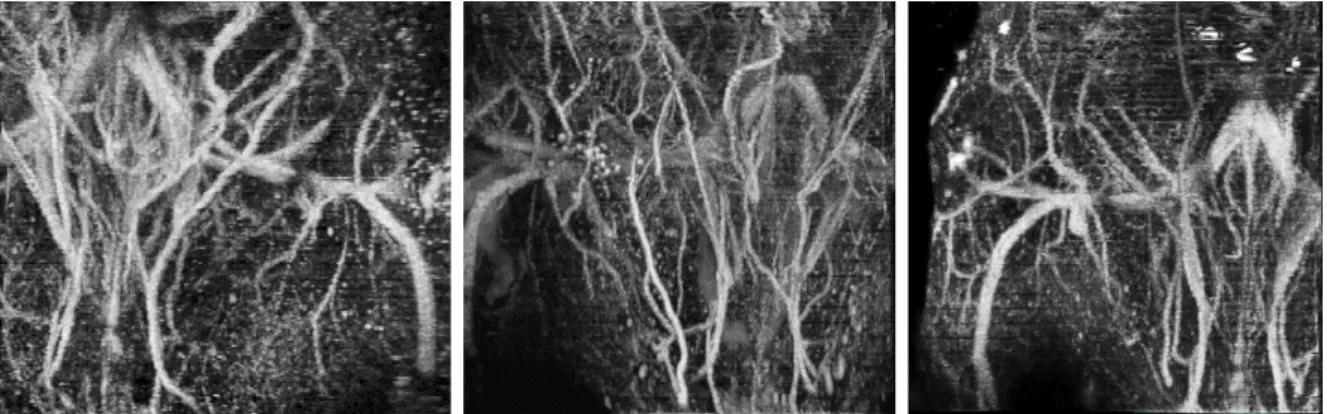
neovasculature, stimulated by tumor angiogenesis, produces strong enhancement in contrast-enhanced vascular images, such as figure 4.12. This figure of a tumor almost 2 mm in diameter (visible as a hypoechoic mass indicated by the cyan marker in the B-mode image) shows closely packed vessels in the corresponding dual-frequency contrast images. In the enlarged, cropped image on the right, we see that the dense vasculature includes both resolvable vessel cross sections, as well as sub-resolution vasculature (such as capillaries) which appears as blurry regions of contrast that do not form resolvable vessel structures. Figure 4.13 shows another example of a tumor with vascular density
Figure 4.12: B-mode image showing a hypoechoic tumor approximately 1.8 mm in diameter and the corresponding contrast image image (2D) below with clear vascu-lar density in the tumor region evident. The panel on the right shows an envascu-larged view of the tumor region with densely packed resolvable and sub-resolution vasculature apparent. All scale bars represent 2 mm.
clearly visible in the frames of acoustic angiography data. This figure shows a single tumor, indicated by the yellow crosshairs, reconstructed in the axial, saggital, and coronal planes.
Figure 4.13: Orthogonal views (single slice) of a representative tumor in acoustic angiog-raphy: (a) axial view, (b) sagittal view, (c) coronal view (rotated 90 counterclockwise). Bars = 3 mm.
Reprinted from Ultrasound in Medicine & Biology, Volume 41, Issue 7, Sarah E. Shel-ton, Yueh Z. Lee, Mike Lee, Emmanuel Cherin, F. Stuart Foster, Stephen R. Aylward, Paul A. Dayton, Quantification of Microvascular Tortuosity during Tumor Evolution Using Acoustic Angiography, Pages 1896-1904, c2015, with permission from Elsevier.
voxels, which were considered to contain contrast signal (and thus containing vascula-ture as well). Then the contrast images were converted to binary images based on this threshold, with contrast pixels represented by 1’s and the background represented by 0’s. The vascular density was calculated by taking the ratio of the number of white pixels in the binarized ROI to the total number of pixels within the ROI, and repeated for all the 2D images across the image volume. Control regions in adjacent tissue were selected by translating the tumor ROI laterally by 1.5 times the tumor diameter to a region of non-tumor tissue. The vascular density of the tumor regions was significantly higher than that of normal regions, with means of 43.8 ± 21.5 versus 19.5 ± 18.0, re-spectively (also listed in table 4.3). Significance testing was done using a paired t-test to compare tumor and normal regions in each animal, resulting in p< 0.01.
Table 4.3: Mean and standard deviations of vascular density of tumor and adjacent regions.
4.4 DISCUSSION
This project rests on the hypothesis that the vasculature in tumors is substantially different from normal normal tissue, and that this difference can be imaged and quan-tified using acoustic angiography contrast-enhanced ultrasound imaging. Support for this hypothesis stems from previous work by UNC neurosurgeon Elizabeth Bullitt and work done in Dr. Paul Dayton’s laboratory. Dr. Bullitt’s work in MRA used the same implementation of the distance metric and sum of angles metric that has been presented in this chapter, and her work showed that glioblastoma multiforme (GBM) tumors had more tortuous vasculature than healthy the brain vasculature of healthy in-dividuals [13,84]. The work by Bullitt and Aylward to produce efficient segmentation of tube-like objects, define 3D tortuosity metrics, and characterize tumor and normal tor-tuosity in the brain were invaluable for informing the design and implementation of this project. Additionally, previous work in the Dayton laboratory and collaboration with Dr. Stuart Foster’s laboratory at the Sunnybrook Health Science Centre (Toronto, ON, Canada) led to the development of the confocal, dual-element transducers that were used in this work, and they also showed that superharmonic contrast imaging (acoustic angiography) could be used to measure higher average tortuosity for large, subcuta-neous fibrosarcoma tumors in rats using the same metrics [143, 144]. These preceding studies have enabled the work in this thesis, which is the first demonstration of serial vascular imaging in a spontaneous tumor model (the C3(1)/Tag) and delves deeper into understanding and characterizing vascular morphology in small tumors.
like most non-invasive, in vivo imaging techniques cannot resolve vasculature at this scale (< 30µm) [175, 176]. Therefore, the result that 2-3 mm tumors have elevated tortuosity compared to controls in acoustic angiography images is significant because it indicates that substantial vascular remodeling in vessels larger than 100 µm has occurred by the time tumors are 2-3 mm in diameter. Angiogenesis at the capillary scale can be inferred due to the enhanced contrast signal originating in these sub-resolution vessels (and was quantified as vascular density), but the structure of individual vessels is unknown below the resolution limit. Therefore, the results presented in this chapter reinforce the fact that cancer angiogenesis produces vascular remodeling and abnormal morphology across a wide range of scales, and is not only restricted to the capillary scale.
of the tumor and the surrounding vasculature, it requires an individual to define the tumor location and boundary. On the other hand, the image on the right is a color map indicating each vessel’s sum of angles metric tortuosity value. Vessels shown in yellow have the lowest tortuosity and brighter red vessels have higher sum of angles tortuosity. Since each vessel is color-coded based on its tortuosity metric, no user input is required beyond vessel segmentation. Despite the fact that the tumor location has not been defined in any way, the tumor is highlighted by a predominance of bright red, tortuous vasculature occurring in and around this tumor. Therefore, tortuosity may be valuable for detecting tumors, in addition to the characterizing their structure as was described in this chapter.
Figure 4.14: Segmented vessels are rendered and displayed in a color-map showing dis-tance from the tumor margin (blue) and sum of angles tortuosity (red).
The panel on the right is reprinted, with permission, from SR Rao*, SE Shelton*, PA Dayton. The fingerprint of cancer extends beyond solid tumor boundaries: assess-ment with a novel ultrasound imaging approach. IEEE Transactions on Biomedical Engineering, Vol. 63, No. 5, p. 1082-1086 (2016).
CHAPTER 5
QUALITATIVE ANALYSIS OF IMAGES: A READER STUDY APPROACH
5.1 OVERVIEW