The Sensitivity of Econometric Model Fit under Different Distributional Shapes

(1)

The Sensitivity of Econometric Model Fit under Diﬀerent

Distributional Shapes

Manasigan Kanchanachitra

A dissertation submitted to the faculty of the University of North Carolina at Chapel Hill in partial fulfillment of the requirements for the degree of Doctor of Philosophy in the Department of Economics.

Chapel Hill 2011

Approved by:

Donna Gilleskie, Advisor

Helen Tauchen

David K. Guilkey

Sang Soo Park

(2)

c � 2011

(3)

Abstract

MANASIGAN KANCHANACHITRA: The Sensitivity of Econometric Model Fit under Diﬀerent Distributional Shapes.

(Under the direction of Donna Gilleskie.)

Answers to many empirical economic questions typically involve quantifying the

relation-ship between a set of explanatory variables and an outcome of interest. Such analyses provide

useful statistics (e.g., marginal eﬀects, treatment eﬀects) or allow for meaningful predictions.

Depending on the question, economists may rely on econometric models to provide additional

information, namely the entire density of a random variable, in order to use diﬀerent moments

of the distribution or accurately capture tails of the distribution. This study examines the

ability of several diﬀerent econometric models to explain the distribution of an outcome.

Us-ing a Monte Carlo experiment, I evaluate diﬀerent economic approaches that are frequently

used by economists to deal with distributions that are positive, skewed and long tailed. Each

econometric model is then evaluated for its performance in estimating the expected outcome

and fitting the distribution particularly in the tails. The distribution of future medical care

expenditure is used throughout the paper to exemplify how the shape of the distribution can

aﬀect optimal behavior, such as the purchase of health insurance, when future medical care

(4)

To Mom, Dad, and Pong

(5)

Acknowledgments

The completion of my dissertation was made possible through the support of many individuals.

First and foremost, I am deeply grateful for the my advisor, Donna Gilleskie, for her continued

guidance throughout the entire process. I truly appreciate her advice, patience, and time. I

would also like to thank my committee members, David Guilkey, Helen Tauchen, Sang Soo

Park, and Sally Stearns, for their invaluable guidance, comments and suggestions.

I am also grateful for my family and friends. I would like to thank my friends in the Thai

Student Association at UNC for making Chapel Hill a home away from home. Thank you,

pAdd, pToon, Teau, and Mink for all your help in my dissertation, but more importantly, for

being great friends. Also, thank you to Michael Darden for your support and encouragement

throughout this journey together. My time in Chapel Hill would not have been the same

without you.

Finally, I wish to express my special gratitude to my Mom, Dad, and sister. Thank you for

believing in me and always being there for me. I would not have come this far without your

(6)

List of Tables

2.1 Alternative Distributional Shapes . . . 6

4.1 Predicted y given x: Log Normal DGP . . . 30

4.2 Summary Statistics of y: Log Normal DGP . . . 31

4.3 Comparing the Tails of the Distribution: Log Normal DGP . . . 33

4.4 Oﬀ by at least 5%: Log Normal DGP . . . 35

4.8 Mean Signed Diﬀerence by Decile: Log Normal DGP . . . 39

4.9 Kolmogorov Smirnov: Log Normal DGP . . . 40

4.10 Optimal Choice: Log Normal DGP . . . 40

4.11 Predictedy given x: Heteroscedastic DGP . . . 44

4.12 Summary Statistics ofy: Heteroscedastic DGP . . . 45

4.13 Comparing the Tails of the Distribution: Heteroscedastic DGP . . . 46

4.14 Oﬀ by at least 5%: Heteroscedastic DGP . . . 47

4.16 Oﬀ by at least15%: Heteroscedastic DGP . . . 49

4.18 Mean Signed Diﬀerence by Decile: Heteroscedastic DGP . . . 52

4.19 Kolmogorov Smirnov: Heteroscedastic DGP . . . 53

4.20 Optimal Choice: Heteroscedastic DGP . . . 53

4.21 Predictedy given x: Random Coeﬃcients DGP . . . 57

(9)

4.22 Summary Statistics ofy: Random Coeﬃcients DGP . . . 58

4.23 Comparing the Tails of the Distribution: Random Coeﬃcients DGP . . . 59

4.24 Oﬀ by at least 5%: Random Coeﬃcients DGP . . . 60

4.28 Mean Signed Diﬀerence by Decile: Random Coeﬃcients DGP . . . 64

4.29 Kolmogorov Smirnov: Random Coeﬃcients DGP . . . 65

4.30 Optimal Choice: Random Coeﬃcients DGP . . . 65

4.31 Predictedy given x: Mixture Model DGP . . . 68

4.32 Summary Statistics ofy: Mixture Model DGP . . . 69

4.33 Comparing the Tails of the Distribution: Mixture Model DGP . . . 70

4.34 Oﬀ by at least 5%: Mixture Model DGP . . . 71

4.38 Mean Signed Diﬀerence by Decile: Mixture Model DGP . . . 75

4.39 Kolmogorov Smirnov: Mixture Model DGP . . . 76

4.40 Optimal Choice: Mixture Model DGP . . . 76

4.41 Predictedy given x: Small Sample DGP . . . 78

4.42 Summary Statistics ofy: Small Sample DGP . . . 79

4.43 Comparing the Tails of the Distribution: Small Sample DGP . . . 80

4.44 Oﬀ by at least 5%: Small Sample DGP . . . 81

4.48 Mean Signed Diﬀerence by Decile: Small Sample DGP . . . 85

4.49 Kolmogorov Smirnov: Small Sample DGP . . . 86

(10)

4.51 Predictedy given x: MEPS 2005 . . . 89

4.52 Summary Statistics ofy: MEPS 2005 . . . 90

4.53 Comparing the Tails of the Distribution: MEPS 2005 . . . 91

4.54 Oﬀ by at least 5%: MEPS 2005 . . . 92

4.58 Mean Signed Diﬀerence by Decile: MEPS 2005 . . . 96

4.59 Kolmogorov Smirnov: MEPS 2005 . . . 97

4.60 Optimal Choice: MEPS 2005 . . . 97

(11)

List of Figures

2.1 Alternative Distributional Shapes . . . 7

4.1 QQ-Plot: Lognormal DGP . . . 32

4.2 QQ-Plot: Heteroscedastic DGP . . . 42

4.3 QQ-Plot: Random Coeﬃcients DGP . . . 55

(12)

Chapter 1 Introduction

Analyses of many economic behaviors require that economists quantify the relationship

between a set of explanatory variables and an outcome of interest. The answer to many

questions posed by health economists depend on assumptions about both the determinants and

the distribution of uncertain outcomes such as medical care expenditure. A common question

in health economics might be to understand how an individual’s health aﬀects his medical care

expenditure. While it may be enough to quantify the eﬀects of particular covariates on the

expected or mean outcome, significant insight may be gained if the eﬀects of covariates on the

entire distribution of an outcome can be ascertained.

The answer to many economic questions oftentimes requires information about the

distri-bution of an outcome of interest. Consider an economic decision making problem that involves

uncertainty. A model of optimal health insurance purchase, for example, states that an

in-dividual chooses a health insurance plan to maximize her expected utility. Health insurance

is chosen without knowledge of one’s medical care expenditures which depend on uncertain

future health (and price and utilization).1 The uncertainty of health requires an individual to forecast at the time of the insurance decision the distribution of medical care expenditures.

The decision of an individual to purchase health insurance depends not only on the

individ-ual’s expected medical care expenditure, but also on the distribution of medical care expenses,

particularly in the far right tail. Health insurance is purchased to protect against the low

1_{While future prices of medical care and future shocks to preferences are also unknown, we focus here on}

(13)

probability of (a disastrous health event that requires) high medical care expenditures.

There-fore, correct modeling of the tail of the medical care expenditure distribution is important for

accurately understanding observed health insurance decisions.

Another example of economic decision making where uncertainty plays a role is the

vaccina-tion decision. Whether or not an individual gets a vaccinavaccina-tion for a particular disease depends

on, among other things, the probability of contracting the disease. An individual may choose

to not get vaccinated if she underestimates her probability of contracting the illness, as she

believes that the costs of getting vaccinated exceed the benefits, or, put diﬀerently, the value

of the expected lifetime utility associated with not vaccinating exceeds that of vaccinating.

Again, the implications from incorrectly forecasting the tails of a distribution may lead to

socially suboptimal vaccination decisions.

Even when the entire distribution is not of specific interest to an economist, calculation of

an outcome’s expected value may depend on assumptions about the entire distribution. Policy

makers may care about predicting average expenditures conditional on covariates, and

estima-tion of the marginal eﬀects often requires some assumpestima-tions about the underlying distribuestima-tion

of the outcome. Incorrect assumptions of the underlying distribution may result in inaccurate

estimates.

Approximation of the entire distribution of an outcome variable, however, is often

com-plicated by particular characteristics of the distributional shape. Many variables of interest

to health economists are characterized by nonnegative outcomes, a nontrivial fraction of zero

outcomes, and a positively skewed distribution with a long heavy right tail. Economists have

many ways to deal with these empirical challenges. In the health economics literature,

skew-ness is frequently addressed by two main approaches when estimating the marginal eﬀects of

covariates on an expected outcome or predicting the outcome itself. The most widely used

model is to take a logarithmic transformation of the dependent variable and apply ordinary

least squares (OLS). The estimated results are then transformed back to the original scale to

achieve interpretable results. A second technique is to use generalized linear models (GLM)

that assume a family distribution for the dependent variable. These approaches, among others,

(14)

While taking skewness into consideration, both of these widely used approaches are limited

to estimating the eﬀect of variation in covariates on variation in the shape and location

pa-rameters of an assumed distribution.2 These models do not let the data fully dictate the shape of the distribution (or capture the tail per se), but rather allow the data to fit an imposed

distribution.

To allow the data to influence the outcome’s distributional shape, one may consider less

parametric models that impose minimal distributional assumptions. These models include

con-ditional density estimation and kernel regression, among others. The use of these approaches

in empirical applications is still quite limited mainly due to their current unavailability in

commonly used statistical software packages.

This dissertation explores diﬀerent econometric approaches3 in their ability to fit skewed and heavy tailed positive outcome distributions while also taking into consideration the

tradi-tional concerns of health economists such as the nontrivial fraction of zeros and the

retrans-formation issue. The goals of this paper are threefold. First, I explore how well each model

performs in estimating the first moment. In particular, I evaluate the sensitivity of these

econometric models to outliers. Second, I evaluate how well each model approximates the

true distribution of outcomes, specifically focusing on the tails of the distribution. Third, I

explore the welfare implications of incorrectly modeling the true distribution. The scope of the

alternative models I consider include parametric, semiparametric and nonparametric models

that extend beyond the frequently used tools. These models are evaluated under diﬀerent

data generating processes using Monte Carlo experiments. The findings of this paper inform

researchers on the optimal choice of estimation tool when faced with diﬀerent types of data

distributions and enable a more thorough interpretation of estimation results.

The rest of this dissertation proceeds as follows: Chapter 2 presents relevant background

information and includes a theoretical example, literature review, and econometric model

2_{The OLS method explains the mean,} _µ_{, and variance,} _σ2_{, of an outcome by variations in explanatory}

variables. GLM specifies that the data follow an assumed exponential family density such as gamma and allows variation in the explanatory variable to explain the shape parameter of the assumed distribution.

3_{Throughout the paper, I use the terms econometric approach and econometric model interchangeably to}

refer to all the alternative approaches considered.

(15)

descriptions. Chapter 3 describes the data generating mechanisms and the Monte Carlo

ex-periment process. Chapter 4 reports the results under diﬀerent data generating processes, and

(16)

Chapter 2 Background

In this chapter, I describe an individual’s optimization problem under uncertainty to

il-lustrate how specification of the distribution of an uncertain outcome is an integral part of

economic analysis. I then provide examples from the empirical economics literature that

demonstrate attempts to capture distributions that aﬀect decision making. Lastly, I describe

the econometric tools that I evaluate in this paper in detail.

2.1 Optimal Behavior under Uncertainty: A Theoretical

Ex-ample

An example of an individual’s optimization problem that I use throughout this paper is the

health insurance selection model. Consider an individual who is uncertain about the state

of his future health, and therefore the associated medical care expenditure he is to incur.

Suppose an insurance company oﬀers the individual the option to purchase insurance where

he may select the level of financial coverage which ranges from 0-100%. That is, if an individual

chooses a 70% plan, the insurance company pays 70% of any future medical care expenditures,

while the individual is responsible for the remaining 30%. The premium for the insurance

increases with the level of coverage. Once the individual chooses the reimbursement level, the

insurance company is responsible for that proportion of the realized medical care expenditure.

Assuming utility is a function of wealth, the individual decides on the optimal level of insurance

(17)

Specifically,

max �

U(w−D−αp+αD)dF(D) (2.1)

where w is the individual’s initial wealth, D is the medical care expenditure that is drawn

from a known distribution,F(_·), andpis the insurance premium per percentage of payout. In this simplified model, the individual maximizes his expected utility by choosing the optimal

level of coverage, α, which takes on a value between 0 and 1. Therefore, the optimal level

of coverage, α, depends on his initial wealth, the rate of insurance premium, his level of risk

aversion, and finally, the distribution of medical care expenditure.

The individual purchases health insurance to insure against the low probability of having

a catastrophic health outcome and hence expenditure. Therefore, it should follow that

diﬀer-ent distributional shapes (particularly in the tails) of medical care expenditure, F(D), may

lead to diﬀerent optimal levels of insurance consumption, α. Suppose we have a risk averse

individual who has an annual income of $36,000. He does not know what his annual medical

care expenditure is going to be, but he does know the distribution from which it is drawn

and that the expected expenditure is $2,500.1 To demonstrate the implications of diﬀerent distributional shapes on an individual’s optimal choice, I hold the expected annual medical

care expenditure constant at $2,500, and vary the degree of skewness and kurtosis. I specify

four separate distributional shapes, all following a gamma distribution to restrict the support

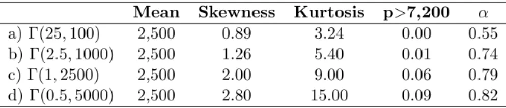
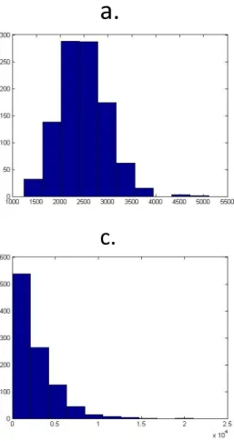
to [0, ∞). All four distributions are positively skewed, as is observed in all empirical data on medical care expenditure, but diﬀer in the degree of skewness and kurtosis. Table 2.1 details

each of the distributions and Figure 2.1 provides the distribution plots.

Table 2.1: Alternative Distributional Shapes

Mean Skewness Kurtosis p>7,200 α

a) Γ(25,100) 2,500 0.89 3.24 0.00 0.55

b) Γ(2.5,1000) 2,500 1.26 5.40 0.01 0.74

c) Γ(1,2500) 2,500 2.00 9.00 0.06 0.79

d) Γ(0.5,5000) 2,500 2.80 15.00 0.09 0.82

1_{The annual income and expected medical care expenditure are based on the 2005 MEPS data for prime age}

(18)









Figure 2.1: Alternative Distributional Shapes

(19)

The four distributions are specified such that they are increasing in the degree of skewness

and kurtosis. When the utility function is specified as u(z) = z0.3, the individual’s optimal choice of insurance coverage is 55% under the first distributional assumption. Increasing

the level of skewness and kurtosis to the second and third distributional assumption, holding

everything else constant, the optimal choice of insurance coverage is 74% and 79% respectively.

Finally, when the distribution is the most positively skewed, the optimal choice of coverage is

highest at 82%.2

The higher degree of kurtosis implies a higher probability that an individual will have a

disastrous health outcome and therefore expenditure. Suppose for the moment that a medical

care expenditure of over 20% of an individual’s income is considered high (in this case, a

medical care expenditure of $7,200 or over). The probabilities of this individual having this

high level of expenditure under the four diﬀerent distributional shapes are 0, 0.01, 0.06, and

0.09 respectively. In other words, if the individual knows that medical care expenditure is

drawn from the first distribution, he knows that he will never receive an extremely high draw

of over $7,200. On the contrary, if his expenditure is drawn from the last distribution with the

highest level of skewness and kurtosis, he has almost a 10% chance of drawing an expenditure

exceeding $7,200. Therefore, the more skewed the distribution (the longer the tail), the more

likely the individual will purchase greater coverage to insure against that increased probability

of facing a disastrous outcome.

2.2 Literature Review of Relevant Econometric Approaches

In this section, I discuss the models and assumptions of three published papers addressing issues

in health economics. Solution of each model requires the econometrician to approximate the

entire distribution of an uncertain variable. I focus on how the researchers attempt to capture

the distribution of a variable of interest, particularly when these distributions are positively

skewed. A review of studies that directly evaluate the performance of particular models is

2_{A less risk averse person would choose a lower level of insurance coverage. For example, if the individual}

(20)

provided in the Model Description section.

I begin with an application to health insurance coverage and employment decisions. Rust

and Phelan (1997) study whether Social Security and Medicare aﬀect an individual’s decision

to retire, when the loans, annuities, and health insurance markets are incomplete. Individuals

realize that there is a positive probability of incurring high medical care expenditures, and there

may be some security value to remaining employed until they are eligible for Medicare. In order

to capture the distribution of medical care expenditures, the authors treat the expenditures

as a mixture of a mass point of $500 or less (to represent the high probability of incurring

some health expenses), and a continuous long tail distribution of the medical care expenditure

over $500. They find that the continuous part is well described by the Pareto distribution,

which has one parameter that characterizes the size of the tail. Their estimates yield a small

parameter value for the Pareto distribution, implying a rather large and long tail translating

to a relatively high probability of having a catastrophic medical care expenditure. Taking

into consideration the uncertainty of medical care expenses, the paper finds that employed

individuals entitled to Social Security benefits are significantly less likely to continue working

as compared to those not entitled to the benefits.

Another study on health insurance and employment decisions examines the employment

behavior of married couples who face uncertainty about future medical expenses (Blau and

Gilleskie, 2006). Again, having health insurance helps couples smooth out their future utility

of consumption across all possible scenarios. The medical care expenditure for each spouse is

assumed to be a random draw from a known distribution. The authors model this underlying

continuous distribution by using a discrete approximation. Specifically, they discretize the

medical care expenditure into three categories (in 1992 dollars): $0-1999, $2000-14,999, and

$15,000 and above, and use multinomial logit models to estimate the probability of being in

each category separately by sex and health status, with an intercept and a linear age term.

The findings suggest a relatively modest impact of health insurance on employment behavior,

given the uncertainty of medical care expenses.

A final example of decision making under uncertainty involves fertility behavior. Infant

mortality is a source of uncertainty that may aﬀect a woman’s fertility decisions. Mira (2007)

(21)

studies the links between infant mortality and fertility decisions when there exists unobserved

heterogeneity in infant mortality risks across mothers. In this dynamic stochastic model of

life-cycle marital fertility behavior, the author focuses on mothers’ learning about their own infant

mortality probability after experiencing child deaths. The paper assumes infant deaths

condi-tional on birth are independent Bernoulli trials with a time-varying, mother-specific probability

of death. Using this framework, the findings suggest that women who experienced higher

in-fant mortality have a higher probability of having additional births as an attempt to replace

the children lost.

These are just a few examples where information about a distribution is necessary for

solution to the optimization problem. The assumptions made by a researcher in estimating

the distribution is likely to impact optimal decisions. In order to evaluate the importance of

distributional assumptions, I consider alternative models that capture the distribution of an

outcome, as well as those that applied economists use to estimate the expected value of the

outcome. I describe these models below.

2.3 Empirical Model Description

Throughout this section, consider an example where the outcome of interest (y) is medical

care expenditures. Possible right hand side variables include sex, age, health status, marital

status, education level, income, etc. I first describe models that deal with the nontrivial

proportion of observations with zero medical care expenditures. In the econometrics literature,

the zero observations are typically handled using one of these models: the two-part model

(2PM) or the sample selection model (SSM). Then I discuss the ongoing debate on choice

between 2PM and SSM. Lastly, I describe models that deal specifically with positively skewed

distributions. These are the econometric models that I implement and evaluate in the Monte

(22)

2.3.1 Two-Part Model

A two-part (or multi-part) model separates the observed positive outcome into two observed

parts: y >0 andy_|y >0. There are two separate equations to directly model these two parts. The first part estimates the probability of observing positive medical care expenditures,y >0,

on the entire example. The first equation is typically estimated using a standard probit model

I =α0+xα1+e1, where e1∼N(0,1) (2.2)

and wherey >0 ifI >0 and y= 0 otherwise.

The second part of the model is estimated on those with any medical care expenditures,

y|y > 0. Typically, the positive outcomes are estimated using OLS on the log transformed variable or GLM. These techniques are discussed separately in subsequent sections.

2.3.2 Sample Selection Model

Following Leung and Yu (1996), I focus on van de Ven and van Praag’s (1981) version of

the adjusted Tobit model. Again, there is a binary variable indicating positive medical care

expenditure commonly modeled using a standard probit. However, the adjusted Tobit model

takes into account the correlation between the probability of any medical care expenditure and

the level of expenditure. There are two equations where the first governs whether y >0 or y

= 0 is observed, and the second governs the level. Specifically,

I =α0+x1α1+e1 (2.3)

m=β0+x2β1+e2 (2.4)

where ln(y) =m ifI >0 and -∞otherwise, and

(e1, e2)∼N

  

 

 0

0  

,

 

 1 ρσ

ρσ σ2

  

 

.

The estimation methods that are most widely used are Heckman’s two-step estimator and

(23)

maximum likelihood. The first method augments the OLS regression with an omitted regressor

ˆ

λ=λ(x1βˆ1). Therefore, using all observations withI >0, the OLS equation becomes

ln(y) =β0+x1β1+ρσλˆ+� (2.5)

where ˆλ=φ(x1αˆ)/Φ(x1αˆ) is the estimated inverse Mills’ ratio. φ(·) and Φ(·) are the p.d.f. and

c.d.f. of the standard normal distribution respectively, andE(�|I >0)=0. For the maximum likelihood method, the likelihood function is given byL= Π0[1−Φ(x1β1)]∗Π1Φ((x1β1+ρ(m−

x2β2)/σ)(1−ρ2)−1/2)φ((m−2β2)/σ)/σ, where Π0 and Π1 are the products over the censored

and uncensored respectively. The method I use in this paper is Heckman’s two-step estimator.

Note that in the 2PM, the decision to have any medical care expenditure (e.g., whether

to see a physician) is independent from the level of expenditure incurred (e.g., how often to

see a physician). Therefore, the estimated level of expenditure is conditional on having any

expenditures. On the contrary, the estimate from the level equation is an unconditional one.

This fundamental diﬀerence between these two models lead to diﬀerent interpretations of the

estimated coeﬃcientsβ.

There has been an ongoing debate on the choice between a two-part model (2PM) and

sample selection models (SSM). A fundamental question involves how one should treat the

nontrivial fraction of zero outcomes. Specifically, are the zeros a result of a random process

or a sample selection process? If the zeros appear random, then the use of a 2PM may be

appropriate. On the other hand, if the observed zero outcomes are likely to be based on

individual choice, then the use of SSM may be more appropriate in correcting for the selection

bias.

The debate started when Hay and Olsen (1984) criticized Duan et al. (1983)’s paper that

compared alternative models for the demand for medical care. In the paper, Duan et al. (1983)

evaluate the performance of a simple one part model, a two-part model, and a four-part model.

Their results suggest that the multi-part models significantly outperform the simple one-part

model in terms of mean squared forecast errors with the four-part model being the most

(24)

the model joint distribution and functional form. Moreover, the multipart model is nested in

the more general selection model.

Duan et al. (1984) respond to the criticism claiming Hay and Olsen (1984)’s proof relies on

an unmentioned restrictive assumption that cannot be satisfied. The authors demonstrated

their point by oﬀering a counterexample to prove that the 2PM is not nested within the SSM.

Duan et al. (1984) further argue that the SSMs are intrinsically flawed since they rely on

untestable assumptions.

Manning et al. (1987) attempt to settle the discussion by using Monte Carlo simulations

to compare these two approaches. Using SSM as their theoretical benchmark, they find that

2PM outperforms SSM on statistical grounds. However, the Monte Carlo design of Manning

et al. (1987) may have created collinearity problems that bias the results against SSM (Leung

and Yu, 1996). The authors argue that if there is no collinearity, SSM would perform much

better than 2PM. Leung and Yu (1996) conduct a diﬀerent set of Monte Carlo experiments to

compare the performance of sample selection and two-part models. They hypothesize that the

reason that the 2PM performs well even when SSM is the true model is due to a subtle design

problem in the simulation experiments. The authors believe that the range of a distribution

which the regressors are drawn from in Manning et al. (1987) are far too narrow. SSM includes

the inverse Mill’s ratio, which is a function of the regressors. Therefore, when the range of

the regressors is not wide enough, the SSM will be burdened with collinearity problems. The

findings from Leung and Yu (1996) suggest that no model outperforms the other under all

conditions.

I now describe models that deal with outcomes that are positively skewed.

2.3.3 Ordinary least squares on log-transformed dependent variable

The ordinary least squares (OLS) on a log-transformed dependent variable is by far the most

prevalent modeling approach used in labor and health economics. The method is simply to log

transform the positively skewed medical care expenditures to ln(y) before applying ordinary

least squares. If ln(y) has a normal distribution with mean µ = xβ and variance σ2_{, the}

(25)

regression model is simply:

ln(y) =xβ+e (2.6)

wherexis a matrix of observed covariates,βis a column vector of coeﬃcients to be estimated,

and eis the error term (Norton, 2007). Note that the error term need not be i.i.d.

The expected value of the logged expenditure is

E(ln(y)) = E(xβ+e)

= xβ.ˆ (2.7)

The log medical care expenditures need to be retransformed back to its original scale to get

interpretable results. If homoskedasticity and normal error terms are assumed, the predicted

retransformed medical care expenditure given the explanatory variables is

E(y) = exp(xβˆ+.5ˆσ2). (2.8)

However, the assumption of normality is quite strong and may lead to inaccurate estimates

ofy. Duan (1983) developed a way to estimate the retransformed dependent variable without

imposing the normality assumption by using a smearing factor, which is the average of the

exponentiated estimated error terms. The predicted medical care expenditure without the

normality assumption is

E(y) = exp(xβˆ)(1 N

n �

i=1

exp(ˆe)). (2.9)

To obtain the marginal eﬀect of xon the raw-scale medical care expenditure y, the

calcu-lation depends on the characteristics of the error terms. The estimated marginal eﬀect of x

is

∂E(y)

∂x = ˆβE(y) (2.10)

where E(y) is from Equation (2.8) or (2.9), depending on whether or not the error term is

assumed to be normal.

(26)

Mullahy, 2001). However, if the log-scale error term is heteroscedastic, then the estimates can

be appreciably biased. To solve for this potential bias, a heteroscedastic retransformation can

be employed (Duan, 1983).

2.3.4 Generalized Linear Model

In generalized linear models (GLM), one directly specifies the mean and variance functions for

the observed medical care expenditure conditional on the covariates. The mean function for

medical care expenditure is represented as

E(y_|x) =µ(x�β) (2.11)

where µ is the inverse link between the expectation of the medical care expenditure and the

linear predictorx�β. The log-link relationship is often chosen in health economics for the mean

function such that

ln(E(y)) = x�β

E(y_|x) = exp(x�β). (2.12)

One also specifies the variance function in GLM. The general form of the variance function

is specified as

ν(x) =κ(µ(x�β))λ (2.13)

whereλmust be nonnegative. The variance is constant whenλ= 0, proportional to the mean

(Poisson-like) if λ= 1, and proportional to the mean squared (gamma-like) if λ= 2.

GLM’s main advantage is that one can directly specify how the expectation of medical care

expenditure in its original scale is related to the covariates. If the link function is correctly

specified, then the choice of the variance function will only aﬀect the eﬃciency. However, if

the link function is misspecified, which may likely be the case, then the model may not fit

the data well across the entire range of the distribution. In this case, the specification of the

variance function will determine the goodness of fit in the diﬀerent parts of the distribution.

(27)

Manning and Mullahy (2001) compare log normal models and gamma models under

dif-ferent data generating specifications based on a Monte Carlo simulation. OLS with a

ho-moskedastic retransformation was more robust than GLM alternatives to heavy-tail data and

large log-scale error term variance. However, the estimates from OLS with a

homoskedas-tic retransformation can be substantially biased if the log-scale error term is heteroscedashomoskedas-tic.

GLM methods also perform better than OLS in terms of precision when the distribution of

the dependent variable is not bell-shaped or skewed bell-shaped.

2.3.5 Three Parameter Generalized Gamma

The three parameter generalized gamma (GG) has one scale parameter and two shape

param-eters. Following Manning et al. (2005), the probability density function for the generalized

gamma is

f(y;κ, µ, σ) = _σy√γ_γγ_Γ(_γ₎exp[z√γ−u] y≥0 (2.14)

where γ = |κ|−2, z = sign(κ)[ln(y)−µ]/σ, and u = γexp(|κ|z). The parameter µ is set to equal x�β. Estimation is done using maximum likelihood methods. The expected value of y

conditional onx for the generalized gamma is

E(y_|x) =exp[xβˆ+ (ˆσ/ˆκln(ˆκ2) +ln(Γ[(1/κˆ2) + (ˆσ/κˆ)])₋ln(Γ[1/ˆκ2])) (2.15)

where ˆσ = (1/n)�exp[α0+α1ln(f(xi))] ifln(σ) is parameterized asα0+α1ln(f(x)).

Manning et al. (2005) extend the Manning and Mullahy (2001) paper by including the

generalized gamma. The Monte Carlo experiment in the paper suggests that the generalized

gamma yields estimates that are close to the true value on the log scale, except for when the

error term is heteroscedastic. The precision loss associated with the generalized gamma is also

smaller compared to GLM of gamma with a log link, which is a special case of the generalized

gamma, when estimating a distribution with heavy tails. However, generalized gamma tends

(28)

2.3.6 Singh Maddala

The Singh Maddala (SM) distribution is also designed to handle heavy tail data distribution.

The density function for the Singh Maddala distribution is

f(y;τ, θ, λ) = λθ λ_{τ y}τ−1

(θ+yτ₎λ+1. (2.16)

One can allow either the shape parameter and/or location parameter to vary with covariates.3

The parameters are estimated via maximum likelihood.

McDonald (1984) finds that the Singh-Maddala distribution provides a better fit for the

income distribution than the gamma, while the gamma outperforms the lognormal. The

paper considers two generalized beta distributions. In particular, the generalized gamma and

generalized beta of the first and second kinds and their special cases were fit to U.S. family

nominal income for 1970-1980. The author finds that the generalized beta of the second kind

provides a better fit than the generalized gamma in terms of sum of squares or absolute errors,

chi-square and log-likelihood criteria. The second best distribution function is Singh-Maddala,

which performs better than the generalized beta of the first kind with four parameters.

2.3.7 Conditional Density Estimation

The conditional density estimation (CDE) approach is based on Gilleskie and Mroz (2004).

Suppose we have some unknown distribution function for medical care expenditures y

condi-tional on a set of covariates x. Let the density of this distribution be f(y_|X). We can break the range of the observed medical care expenditures intoK intervals, where the kth interval is

defined by [yk−1, yk), foryk−1≤yk,y0 =−∞ and yK =∞.

The conditional probability that an observed value of medical care expenditure falls in the

kth interval given that it did not fall in one of the first (k-1) intervals is

λ(k, x) =p[yk−1 ≤ y < yk−1] =

�yk

yk−1f(y|x)dy

1−�yk−1

y0 f(y|x)dy

. (2.17)

3_{The SM density function from Stata is}_f₍_x_;_{a, b, q}_{) = (}_aq/b₎_z−(q+1)_[(_x/b₎(a−1)_]

(29)

Therefore, the probability that the random variable y falls in the kth interval is given by

p[yk−1 ≤ y < yk|x] =λ(k, X)

k_�−1

j=1

[1−λ(j, x)]. (2.18)

The true expectation of any functionh(·) of the random variabley given x, is

E(h(y)_|x) =

� _∞

−∞

h(y)f(y_|x)dy (2.19)

whereh(·) is any smooth and continuous function ofy.

The discrete approximation of the expected function using a partition of the support of y

withK intervals is given by,

˜

E(h(y)_|x) = K �

k=1

h∗(k_|K)λ(k, x) k_�−1

j=1

[1₋λ(j, x)], (2.20)

where each h∗(k_|K) is an approximation to h(y) in the kth interval. Gilleskie and Mroz are interested in the mean of y and therefore let h∗(k|K) be the mean or the arithmetic average function, which does not vary with the x’s. This implies that, conditional on being in that

interval, the x’s do not explain the mean value within their interval. That is, conditional on

being in a particular interval, the value of y is random. The derivative of the conditional

expected value in this case is

∂E˜(h(y)_|x)

∂x =

K �

k=1

h∗(k_|K)∂[λ(k, x)

�k₋1

j=1(1−λ(j, x))]

∂x (2.21)

One could also allow the mean to depend onx’s. Ifh∗(k_|K) varied withx, the derivative of the conditional expected value would have an additional term that reflects the fact thath∗(_·) is also a function of x. Their paper suggests however, that the proposed conditional density

estimator performs quite well under various data generating processes. More importantly, this

estimation method allows effects of covariates to be different at different points of support in

(30)

2.3.8 Kernel Regression

Kernel regression is a nonparametric technique that is less dependent on functional form

as-sumptions than parametric models (Yatchew, 1998). Consider a modely=f(x) +e, where e

is i.i.d. with mean 0 and variance σ2

e given x, whichx is assumed to be a scalar for the time

being. The functionf is unknown. A general formulation of local averaging estimator can be

defined as

ˆ f(x0) =

�

wt(x0)yt. (2.22)

Several local averaging estimators can be used including kernel and nearest neighbor. Higher

weights are assigned to observations closer tox0.

I focus on the kernel estimators. The weight function is specified as

wt(x0) = 1

λTK(

xt−x0

λ )

1

λT �

K(xt−x0

λ )

(2.23)

whereKis assumed to be a bounded function that sums to one and is symmetric around zero.

It determines the shape of the weights and the magnitude is determined by the bandwidth,λ.

The larger the bandwidth, λ, the more weight is being put on observations that are far from

x0. The kernel regression function estimator is therefore

ˆ f(x0) =

1

λTK(xt−λx0)yt

1

λT �

K(xt−x0

λ )

(2.24)

There are several types of kernels. The simplest form is the uniform kernel which gives

the weight of 1 on [-1/2, 1/2] and 0 otherwise. The kernel that I use in this paper is the

Epanechnikov function which takes the value of 3₂(1−4u2) whereu∈[−1/2,1/2]. The choice of kernel is not as important as the choice of bandwidth size. The mean squared error can be

minimized by increasing the bandwidth of the neighborhood until the increase in bias squared

is oﬀset but the decrease in variance.

Nonparametric regressions are not as widely used as one might expect. The main reasons

are that the nonparametric techniques are more complex than procedures available in

stan-dard statistical software packages, they are computationally intensive, and they require large

(31)

datasets.4

2.3.9 Finite Mixture Model

The finite mixture model (FMM) uses a mixture of distributions to approximate the true

un-known distribution. The FMM can accommodate heterogeneity between diﬀerent subgroups

of individuals such as heavy users and light users of medical care. With the FMM, the

distri-bution ofyis assumed to be drawn from a population that is an additive mixture ofC distinct

subpopulations in proportions π1,...,πC, where �Cj=1πj = 1, and πj >0. The density of y is given as

f(y|Θ) =π1f1(y|θ1) +...+πCfC(y|θC) (2.25)

where fj(y|θj)’s are specified to follow a distribution such as normal or Gamma. The mixing probability parameters, πj, are estimated along with other parameters of the distribution,

θj via maximum likelihood. In this paper, I specify the distribution to be a mixture of two

Gamma distributions.

Deb and Holmes (2000) compare the performance of FMM to the two-part count model in

estimating visits, and to the two-part model with OLS on log transformed dependent variable

in estimating medical care expenditures. Using data from the National Medical Expenditure

Survey, the authors conclude that the FMM provides a better fit of both visits and expenditures

than the standard models. Their results indicate that there is heterogeneity in the population

that can be classified into at least two diﬀerent subgroups with diﬀerent density parameters.

The FMM is able to capture this diﬀerence between the subgroups, categorizing users into high

intensity user group, and low intensity user group. The high intensity user group is found not

only to have a higher expected expenditures, but also a higher variance than the low intensity

user group.

4_{The more regressors there are in the model, the larger number of observations is needed as Kernel regression}

(32)

Chapter 3 Monte Carlo Experiment

To evaluate the performance of alternative econometrics models, I implement a Monte Carlo

experiment. I generate datasets such that there exists a nontrivial proportion of the sample

with zero observed outcomes and for those with positive outcomes, the data are right skewed.

I consider diﬀerent data generating processes to reflect common features in health economics

data. Specifically, I start with a basic dataset where the positive part of the dependent variable

yfollows a log normal distribution. I then add in heteroscedasticity in the log-scale error term

for the second data generating process. The third data generating process I consider is specified

to have random coeﬃcients, while the last data generating process is based on a mixture of

distributions. In addition, I also consider a small sample dataset. The specifications of each

of the data generating processes are detailed below.

3.1 Data Generating Processes

The first data generating process (DGP) is a two-part model where the positive part of the

distribution is based on a lognormal. The first part dictates the probability of an individual

having any positive medical care expenditure and is specified as

(33)

wheree1 ∼N(0,1). IfI ≤0, then the individual has no medical care expenditure and y= 0.

IfI >0, then the individual has a positive expenditure which is determined by

ln(y) =β0+β1x+e2, (3.2)

where x∼ Γ(3.4,0.24), e2 ∼N(0,1), and e2 is uncorrelated with e1. In this data generating

process, α0, α1, β0, andβ1 are specified to be 0.06, 1.00, 5.85, and 1.74 respectively.1 I is the

indicator function for having any positive expenditure,yis the medical care expenditure given

I >0, andx is an explanatory variable such as health status, and therefore x is positive and

its distribution is skewed right. In this example, higher values ofx indicate worse health. The

summary statistics for this lognormal DGP are provided in Chapter 4 in Table 4.2.

The second data generating process incorporates heteroscedasticity in the error term, which

is a common feature in health economics data. This DGP is similar to the baseline lognormal

DGP in that it is also a two-part model, andx_∼Γ(3.4,0.24). Similarly, the error terms from the first part and the second part of the model are not correlated. However, the second part

of the model that predicts the level of expenditures conditional on having any expenditures is

heteroscedastic in the error term. The variance of the error term is specified to be a function

of x. Specifically, e2 ∼ N(0,1 +x/5). Under this DGP, the values for α0, α1, β0, and β1 are

-0.01, 1.00, 5.48, and 1.74 respectively. The summary statistics for this heteroscedastic DGP

are in Table 4.12.

The third data generating process is also similar to the first DGP but the coeﬃcient in

the second regression function, β1, is random. In particular, β1 is drawn from a N(1.74,0.5)

distribution. Other parameters, α0, α1, and β0 are set to be -0.025, 1, and 5.28. Table 4.22

provides the summary statistics of this heterogeneous DGP.

To reflect the fact that most data do not follow any one particular distribution, the next

1_{In all my data generating processes, I adjust the coeﬃcients so that the mean medical care expenditure is}

(34)

case I consider is when the distribution of the outcomes is a mixture of models. Specifically,

the DGP is a mixture of two lognormal distributions. Individuals are randomly assigned to

be one of two possible types. The two types have diﬀerent probabilities of incurring any

positive expenditures, and upon having any expenditures, the mean levels of expenditures are

diﬀerent. One can typically think of these “unobserved” types as relatively healthy individuals

versus relatively unhealthy individuals. The relatively healthy individuals, on average, have

a lower chance of having any expenditures than their relatively unhealthy counterpart, and

conditional on having any expenditures, the relatively healthy individuals can expect to have a

lower expenditure. In my specification, I have approximately 70% of the population being the

relatively healthy type, and the remaining 30% being the relatively unhealthy type. Within

each type, the error terms in the first and second part of the model are correlated. For the

relatively healthy individuals, the parameters α0, α1, β0, and β1 are set to be -0.009, 1.00,

5.2, and 1.4 respectively, while the relatively unhealthy individuals, the parameters are set as

0.15, 1.00, 6.2, and 1.74. Under this specification, the average probability of having positive

expenditures for the relatively healthy individuals is 0.77 and conditional of having positive

expenditures, the expected expenditure is $2,583.08. A relatively unhealthy individual, on the

other hand, has a higher probability of having any positive expenditures of 0.82, and upon

incurring any expenditures, the expected expenditure is also higher at $6,717.44. The details

of the entire distribution are shown in Table 4.31.

Finally, I consider a small sample DGP. Specifically, the DGP is the same as the one with

a heteroscedastic error term but with a considerably smaller sample size. The sample size in

all other DGP is 10,000, while the small sample DGP, the sample size is 1,000.

After evaluating the various econometric approaches under diﬀerent DGP’s, I implement

these models using a real dataset. The dataset that I use is the 2005 Medical Expenditure

Panel Survey. I discuss the details of the data in Section 4.6.

(35)

3.2 Experiment Design

To begin the Monte Carlo experiment, I generate 10,000 observations following the data

gen-erating processes described above. For each DGP, I use each of the considered estimating

approaches to attain the predictedy given the values ofx.

The main goal of this paper is to evaluate the performance of each of the econometric

models in terms of distributional fit, in addition to the predicted value of y given x. In order

to fulfill this goal, I need to recover the simulated distribution of y as implied by each of the

econometric models, and compare this simulated y to the actual data that I have generated.

Suppose yi =f(xi) +ei is the observed yi from the DGP. The simulated outcome, ˜y, is then

defined as ˜y= ˆf(xi) + ˜ei where ˆf(xi) incorporates estimates from the model and ˜ei is obtained

from simulating the error terms. For example, after using OLS on log-transformed y, I have

ˆ

f(xi) asxiβˆ. I then generate ˜yi by adding an error term, ˜ei, that is drawn fromN(ˆµ,ˆσ2) where ˆ

µ and ˆσ2 are found in estimation. I then transform the distribution back to its original (not log) scale. Note that I assume that the error term from OLS follows a normal distribution.

However, I am not able to simulate the error terms for all models, particularly those that

are nonparametric. I describe the process by which I generate the simulated y from each

econometric model in detail in Appendix A.

The simulation process is repeated 50,000 times to achieve 50,000 sets of ˜y for each

econo-metric model under each DGP. Each set of ˜y’s from each round of simulation is then sorted in

ascending order. Then I take the average of the ˜y₍_i₎ (where ˜y₍_i₎ is theith order statistic of the sample) across simulations to obtain the final set of ˜y’s that I use in my evaluations.

3.3 Evaluation Criteria

The performance of each econometric model is evaluated in three main aspects:

• Predicted y given x. Each model is compared in how well it predicts the mean.

(36)

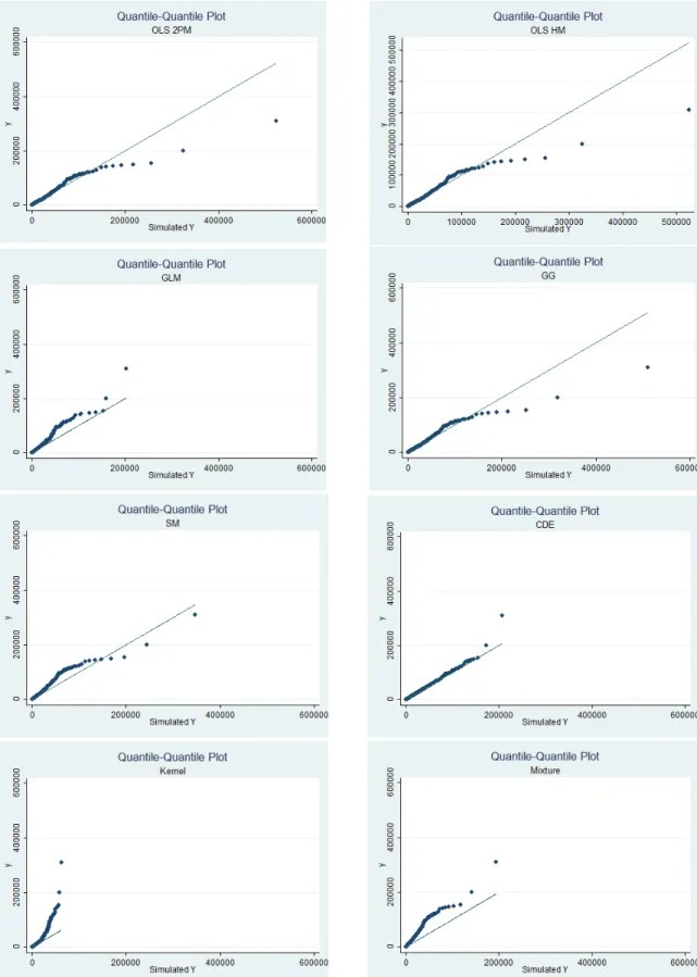
– qq-plot. The first criterion to evaluate the overall fit of the models is to plot the

simulated outcome, ˜y, against the true data that are generated,y, at each quantile.

The qq-plot is useful particularly in examining the model fit in the extreme right

tail. The simulated and actual values are first sorted from the lowest to the highest,

then are plotted against one another. If a model fits the data perfectly, the qq-plot

should be a 45 degree line. That is, the simulated values are equal to the actual

values. The more the qq-plot deviates from the 45 degree line, the worse the fit.

If the qq-plot is above the 45 degree line, the model underpredicts the data, and

overpredicts if the qq-plot is below the 45 degree line. Therefore, the qq-plot is a

good gauge for each model’s performance across diﬀerent values of y.

– Percentage oﬀ by decile. This criterion is used in conjunction with the qq-plot.

Once both the simulated and actual values are sorted from lowest to highest, they

are compared to one another. I calculate the percentage that the simulated values

diﬀer from the true values. That is, for eachy₍_i₎and ˜y₍_i₎, I calculate (˜y₍_i₎₋y₍_i₎)/y₍_i₎. I report the percentage of observations that are oﬀ by at least 5%, 10%, 15%, and

20%. Note that I calculate the percentage for positive values ofy. That is, I report

the percentage conditional ony >0.

– Mean Signed Diﬀerence (MSD) by decile. The MSD is also to be used in conjunction

with the qq-plot. The MSD is defined as MSD = �N_i₌₁(˜y₍_i₎−y₍_i₎)/N, and it is intended to assess the direction of the fit on average in each part of a distribution.

In other words, the MSD reports whether the simulated distribution on average

under- or overpredicts the true distribution. The closer the MSD to zero, the

better the fit. If the MSD is negative, that means on average the values of the

simulatedy in that decile are smaller than the true values. A positive MSD means

that on average, the simulated y’s are above the true y’s. I report MSD1-MSD10

corresponding to the first to the tenth deciles. Note that these deciles are based on

the positive values ofy to be consistent with the percentage oﬀ by decile criterion.

I also include MSD0 for the case where y is equal to zero.

(37)

– Percent greater than cutoﬀ point. This criterion is used as a rough gauge in how well

the simulated distribution fits the right tail of the true distribution. I choose a y

cutoﬀ point in the true distribution, and calculate the percentage of the observations

that lie above that cutoﬀ point. I then calculate the percentage of observations that

lie above this same cutoﬀ point in the simulated data. The percentages are then

compared.

– Kolmogorov-Smirnov Statistic. The KS test is a fully nonparametric test that

com-pares the distribution of the simulated outcomes to the distribution of the

ob-served data. It determines whether the two underlying distributions diﬀer. The

KS test statistic is D = max(|D+|,|D−|), where D+ = max(F(˜y)−F(y)) and D− = min(F(˜y)−F(y)). The KS test measures the vertical distance between the cumulative distribution of the simulated outcome, ˜y, and the cumulative

distribu-tion of the observed outcome,y. The KS test can evaluate the distributional fit of

each model without imposing any distributional assumptions.

• Welfare implications. The distributional shape as implied by each of the models may have welfare implications in models of decision making under uncertainty. To analyze

the implications of a model’s performance in fitting a distribution, recall the health

insurance optimization problem in Equation 2.1 of Chapter 2. The simplified model

states that an individual, uncertain of future health and therefore medical care expense

(D), chooses a level of insurance coverage (αfrom 0-1, where α is the proportion of any

future medical care expenditures that the insurance company is responsible for, and 1-α

is the proportion that the individual is responsible for) to maximize his utility which is

a function of wealth, w. I create a scenario where the individual has an initial wealth

of $18,0002_{; the premium per unit of coverage,} _p_{, is $10; and the individual’s utility}

function is specified as U(z) =zr_{, where} _z ₌_w₋_D₋_αp₊_αD_{, and} _r _{is set to 0.8 to} reflect risk aversion. The optimization problem is solved by discretizing the simulated

outcome distribution and it is solved by using Mata in Stata. The optimal choices

(38)

under uncertainty, where the distribution of medical care expenditures is estimated using

each econometric approaches, are then compared to the optimal choice under the true

distribution.

(39)

Chapter 4 Results

In this Chapter, I discuss the performance of each econometric models under diﬀerent data

generating processes using the evaluation criteria as described in Chapter 3.

4.1 Lognormal Data Generating Process

I begin with the performance of each econometric model under the lognormal DGP. Most

models perform quite well in predicting the mean under this simple lognormal DGP. SM and

the FMM are the only models that are inaccurate in predicting the mean. See Table 4.1 for

each model’s predicted mean.1

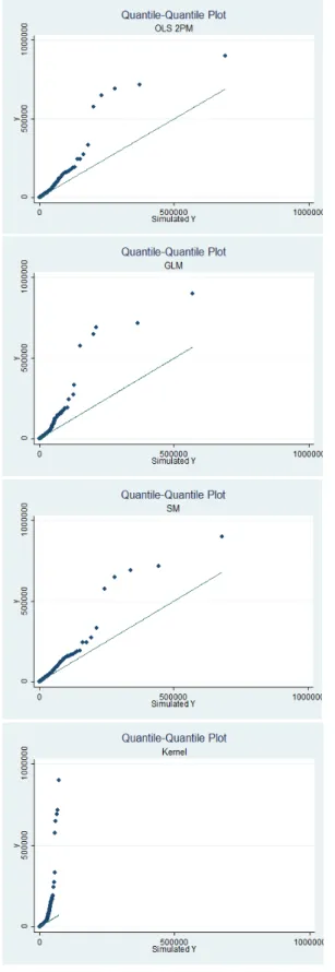
To evaluate the distributional fit of each model, let us begin by looking at the summary

statistics of the true distribution and the simulated distributions. Table 4.2 provides the

summary statistics of the true y and the simulated y from each of the models. In general, all

models fit the mean of the true distribution quite well. The simulated distribution generated

by both OLS models and the GG are very similar. The simulated distributions from these

models are much more skewed and have a higher level of kurtosis than the true distribution,

implying a fatter tail than the true distribution. The GLM’s simulated distribution has similar

skewness and kurtosis to the true distribution, but a lower standard deviation and variance.

1_{Note that the predicted probability of having any positive expenditures (Prob}_{y >}_{0) for OLS TP, SSM,}

(40)

The summary statistics suggest that the simulated distribution from GLM has a similar shape

to the true data, but smaller in scale.

The simulated distribution from Kernel regression compared to the true distribution of

the outcomes is much less skewed and has a much lower kurtosis. The tail of the simulated

distribution from Kernel regression is much shorter compared to the true distribution and the

simulated distributions from other models. It may seem at first that the simulated distribution

from the Kernel regression fits the true distribution quite poorly. However as we will later see,

the simulated distribution from the Kernel regression fits the overall true distribution rather

well, and only in the extreme right tail that the fit is very poor. The maximum simulated

y from the Kernel is 62,098.48, which may seem much lower than the maximum of 309,337.9

from the true distribution, but it corresponds to approximately the 0.996 quantile of the true

distribution. It is the outliers of the true distribution that the simulated distribution cannot

capture, resulting in a simulated distribution with a much shorter right tail.2

SM and FMM both underpredict the mean. Both models have lower standard deviations

and variances, but FMM has a higher level of skewness and kurtosis than the true distribution,

suggesting that the simulated distribution from the FMM has a higher mass in the lower values

of the distribution than the true data. The reason SM and FMM perform poorly in fitting the

true distribution may be due to their underlying distributional assumptions. Both the

Singh-Maddala distribution and the Gamma distribution that the SM and FMM rely on respectively,

have shorter right tails than the lognormal distribution that the true distribution is based

on. This shorter right tail may be the reason in the observed lower standard deviations and

variances in both SM and FMM simulated distributions.

The simulated distribution from the CDE is close to the true distribution, with the

simu-lated distribution being slightly less skewed and has less kurtosis.

Overall, both OLS models and the GG model do well in fitting the entire distribution.

2_{The simulated distribution from the Kernel regression is based on calculating the estimated conditional}

CDF of yand inverting this conditional CDF to obtain the simulatedy. The choice of the bandwidth plays

an important role in how well the simulated distribution fits the true distribution. I use the rule-of-thumb in calculating the size of the bandwidth. If I use a larger bandwidth than the optimal bandwidth that the rule-of-thumb suggests, I would be able to capture the outliers better, but at the expense of over-smoothing the distribution. See Appendix A for further detail.

(41)

(42)

(43)



 

 

(44)

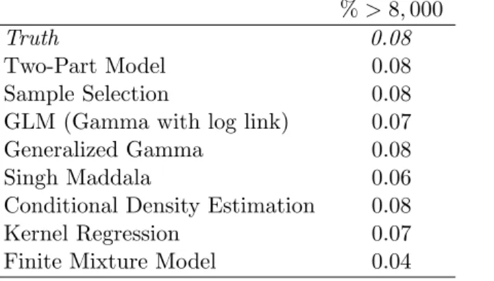
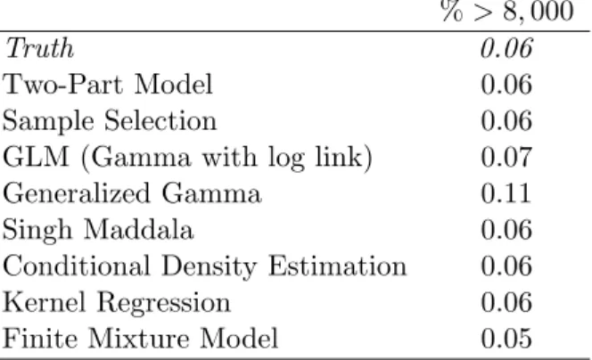
Table 4.3: Comparing the Tails of the Distribution: Log Normal DGP %>8,000

Truth 0.08

Two-Part Model 0.08

Sample Selection 0.08

GLM (Gamma with log link) 0.07

Generalized Gamma 0.08

Singh Maddala 0.06

Conditional Density Estimation 0.08

Kernel Regression 0.07

Finite Mixture Model 0.04

Table 4.4 reports the percentage of the observations in the simulated distribution that are

diﬀerent than the true distribution by at least 5%. For both OLS models and the GG models,

only 2.26%, 3.31%, and 1.19% of the entire simulated distributions respectively, are diﬀerent

from the true distribution by 5% or more. The tail of the distribution, in the tenth decile, is

where most of the diﬀerences come from. From the qq-plots in Figure 4.1 and Table 4.8, it

seems that these three models overpredict the right tail of the distribution.

GLM performs well in predicting the mean. However, its performance in fitting the

distri-bution is not as good. From Table 4.7, 71% of the overall simulated distridistri-bution from GLM

is diﬀerent from the actual distribution by at least 20%. Interestingly, under this DGP the

GLM does not do as poorly in the higher deciles (9th-10th) compared to the lower deciles.

However, compared to both OLS models and the generalized gamma, the GLM still performs

worse. From the qq-plot in Figure 4.1 and the MSD in Table 4.8, it shows that the GLM

underpredicts the far right tail, while consistently overpredicting the rest of the distribution.

Compared to both OLS models and the generalized gamma model, GLM has a much shorter

right tail.

SM does moderately well in terms of its distributional fit compared to other models. The

simulated distribution is generated based on a SM distribution and it should be expected that

it does not fit the true distribution as well as OLS models and GG. From Tables 4.4, 4.5, 4.6,

and 4.7, SM seems to be performing best around the mean. In terms of the right tail, SM

underpredicts the true values. There are also less observations in the distribution of ˜y above

the cutoﬀ point at 8,000 than in the true distribution ofy (see Table 4.3).

(45)

Kernel regression performs well in fitting the true distribution everywhere except for the

right tail. Note that the simulated y’s from Kernel regression is lower than the true y’s

everywhere in the distribution and the magnitude of the diﬀerence is one of the highest (see

Table 4.8). The poor fit in the far right tail of the Kernel simulated distribution also shows

quite clearly in the qq-plot in Figure 4.1. The plot shows how much shorter-tailed the simulated

distribution is compared to the true one.

Examining the qq-plot in Figure 4.1, CDE appears to do quite well. It seems to slightly

underpredict the far right tail of the true distribution. However, upon closer inspection, CDE

fits quite well in the right tail, but most of its poor fit occurs in the left tail as suggested by

Tables 4.4, 4.5, 4.6, and 4.7. The poor fit in the left tail is not clear in the qq-plot.

The model that does consistently poorly is the FMM. It does poorly in predicting the mean

and fitting the distribution. Note, however, that the FMM assumes a mixture of two Gamma

distributions when the true distribution is a lognormal, so the Gamma can fit a lognormal only

to a certain extent. Also note that by construction of this DGP, there is no mixture of models

while I specify the FMM to be a two component model. One should expect a two component

model fitting a one component model to not work as well.

Another evaluation criterion I use to determine the overall fit is the Kolmogorov Smirnov

statistic (KS). Table 4.9 reports the statistics from diﬀerent estimation models. The first

column is the D statistics as explained in Section 3.3. The higher theD statistic, the bigger

the largest vertical distance between the true distribution and the simulated one. The second

column is the p-value of the combined test, and the third column is the corrected. Based on

the KS, the correctedp-value is significant for GG.

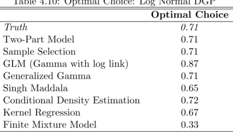
Finally, I examine how the simulated data from each model may aﬀect an individual’s

op-timal behavior. Under the true distribution of medical care expenditures, the opop-timal amount

of coverage for the individual is 0.71 as shown in Table 4.10. That is, the individual chooses

coverage such that the insurance company pays for 71% of any future medical expenses while

he is responsible for the remaining 29%. Both OLS models, GG, and CDE, which perform

well in fitting the distribution, all result in the same optimal behavior. GLM which does

(46)

(47)

(48)

(49)

(50)

(51)

Table 4.9: Kolmogorov Smirnov: Log Normal DGP D P-value Corrected

Two-Part Model 0.017 0.123 0.119

Sample Selection 0.017 0.123 0.119

GLM (Gamma with log link) 0.229 0.000 0.000

Generalized Gamma 0.004 1.000 1.000

Singh Maddala 0.026 0.003 0.003

Conditional Density Estimation 0.099 0.000 0.000

Kernel Regression 0.013 0.415 0.408

Finite Mixture Model 0.112 0.000 0.000

of 0.87. The Kernel regression which fits the overall distribution well except for the far right

tail predicts the optimal behavior at 67%, which is lower than the true optimal choice. In

most part, the tail of the distribution is a good indicator of the optimal choice. If a simulated

distribution underpredicts the tail, then the resulting optimal choice is typically lower than

the true optimum, and vice versa. This relationship between the tail and the optimal behavior

is seen in the SM, Kernel, and FMM models.

Table 4.10: Optimal Choice: Log Normal DGP Optimal Choice

Truth 0.71

Two-Part Model 0.71

Sample Selection 0.71

GLM (Gamma with log link) 0.87

Generalized Gamma 0.71

Singh Maddala 0.65

Conditional Density Estimation 0.72

Kernel Regression 0.67

The Sensitivity of Econometric Model Fit under Different Distributional Shapes

The Sensitivity of Econometric Model Fit under Diﬀerent

Distributional Shapes

Abstract

Acknowledgments

Table of Contents

List of Tables

List of Figures

Chapter 1

Introduction

Chapter 2

Background

2.1

Optimal Behavior under Uncertainty: A Theoretical

Ex-ample









2.2

Literature Review of Relevant Econometric Approaches

2.3

Empirical Model Description

Chapter 3

Monte Carlo Experiment

3.1

Data Generating Processes

3.2

Experiment Design

3.3

Evaluation Criteria

Chapter 4

Results

4.1

Lognormal Data Generating Process