CONTROLLING MULTIPLICITY IN CONFIRMATORY CLINICAL TRIALS
Hengrui Sun
A dissertation submitted to the faculty at the University of North Carolina at Chapel Hill in partial fulfillment of the requirements for the degree of Doctor of Public Health in the department of Biostatistics
in the Gillings School of Global Public Health.
Chapel Hill 2016
ii
iii ABSTRACT
Hengrui Sun: Controlling Multiplicity in Confirmatory Clinical Trials (Under the direction of Gary G. Koch)
Multiplicity is an important statistical consideration that arises in clinical trials when the efficacy of the test treatment is evaluated in multiple ways. The scope of multiplicity includes multiple efficacy endpoints, multiple inferential subgroups, multiple treatments or doses, etc. The major concern for multiplicity is that insufficiently controlled multiple assessments lead to an inflated family-wise (or experiment-wise) Type I error rate (FWER) and they thereby undermine the integrity of the statistical inferences. Therefore, a sound statistical strategy that controls FWER in a strong sense for the multiple assessments, without excessive loss of power (or Type II error) from over-control, is crucial for the success of the trial.
Chapters 1 and 2 explore strategies for multiplicity issues that come from only one source, which may involve strictly ordinal response outcomes, stratified design, baseline imbalances, and missing values. Realistic case examples are provided, and solutions are proposed to address those issues comprehensively.
iv
v
TABLE OF CONTENTS
LIST OF TABLES ... ix
LIST OF FIGURES ... x
CHAPTER 1 : LITERATURE REVIEW AND INTRODUCTION ... 1
1.1 Multiplicity Issues in Confirmatory Clinical Trials ... 1
1.1.1 Multiple Endpoints ... 1
1.1.2 Subgroups ... 2
1.1.3 Multiple Treatments / Doses ... 3
1.1.4 Multiple Visits ... 3
1.2 FWER and Its Considerations in Confirmatory Clinical Trials ... 3
1.3 Overview of the Multiplicity Management Strategies ... 4
1.3.1 Hierarchical Methods ... 4
1.3.2 Basic Bonferroni Procedure and Alpha Propagation Methods ... 5
1.3.3 Closed Testing Procedure through Multiway Averages ... 6
1.3.4 Adjusted P-values for Simultaneous Inference ... 7
1.4 Global Test ... 8
1.4.1 O’Brien’s Global Test ... 9
1.4.2 Generalized Estimating Equations ... 10
1.4.3 Cox Model and the Wei-Lin-Weissfeld Method ... 11
1.4.4 Stratified Mann-Whitney Estimator ... 12
1.5 Handling Baseline Imbalance in Clinical Trials ... 14
1.5.1 Nonparametric Randomization Based ANCOVA ... 15
vi
1.5.3 Dichotomous, Ordinal and Survival Outcomes ... 17
1.6 Innovative Applications ... 17
1.6.1 Global Test ... 18
1.6.2 Multiple Testing Strategy ... 18
1.6.3 Randomized Respiratory Disorder Trial with Four Visits ... 19
1.6.4 Randomized t-PA Stroke Trial with Multiple Outcomes ... 21
1.7 Summary of Research ... 22
REFERENCES ... 25
CHAPTER 2 : ANALYZING MULTIPLE ENDPOINTS ... 28
2.1 Introduction ... 28
2.2 Methods... 29
2.2.1 Stratified Multivariate Mann-Whitney Estimator ... 29
2.2.2 Randomization Based Nonparametric Covariance Adjustment ... 31
2.2.3 Missing Values ... 31
2.2.4 Global Test ... 32
2.2.5 Closed Testing Strategy ... 34
2.3 Randomized Clinical Trial for Osteoarthritis (ACTA) ... 35
2.4 Results ... 35
2.5 Discussion ... 37
REFERENCES ... 43
CHAPTER 3 : MULTIPLE SUBGROUPS WITH MULTIPLE ENDPOINTS ... 44
3.1 Introduction ... 44
3.2 A Real Case Example ... 47
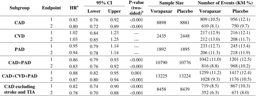
3.2.1 TRA 20P – TIMI 50 trial ... 47
3.2.2 Alternative statistical planning ... 48
3.3 Multiple Testing Strategy ... 50
vii
3.3.2 Extension of O’Brien’s global test ... 51
3.3.3 Closed testing procedure ... 52
3.3.4 Analysis strategy ... 52
3.3.5 Covariance matrix estimation ... 53
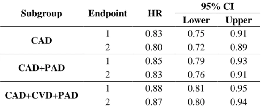
3.3.6 Results for TRA 20P – TIMI 50 trial ... 54
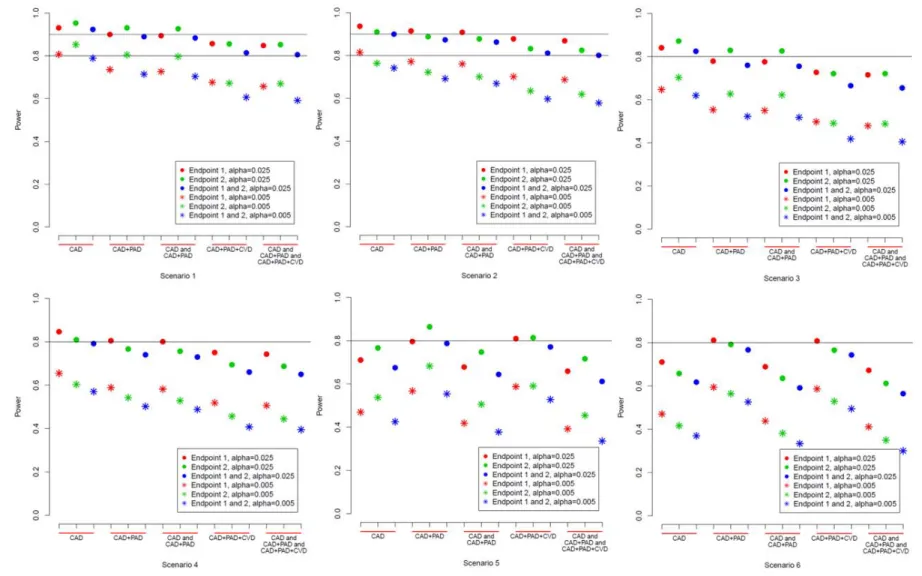
3.4 Simulation and Results ... 55
3.4.1 Simulation planning ... 55
3.4.2 Results ... 56
3.5 Discussion ... 57
REFERENCES ... 74
CHAPTER 4 : MULTIPLE TREATMENTS, VISITS AND ENDPOINTS ... 75
4.1 Introduction ... 75
4.2 An Illustrative Example ... 76
4.2.1 Suvorexant Trials ... 76
4.2.2 Suvorexant Trial Statistical Planning ... 77
4.2.3 Alternative Strategies ... 79
4.3 Modified Statistical Planning ... 80
4.3.1 Global test ... 80
4.3.2 Extension of O’Brien’s global test ... 81
4.3.3 Closed testing procedure ... 82
4.3.4 Multiplicity strategy ... 83
4.4 Results of the Combined Suvrorexant Studies ... 84
4.5 Simulation Study ... 84
4.5.1 Simulation Parameters ... 84
4.5.2 Simulation Results ... 86
4.6 Discussion ... 87
viii
ix
LIST OF TABLES
Table 1.1 Respiratory disorder trial results ... 20
Table 1.2 Published t-PA stroke results. ... 22
Table 1.3 Re-analysis of the t-PA stroke trial ... 22
Table 2.1 Mann-Whitney estimators (95% CI) at baseline ... 39
Table 2.2 Mann-Whitney estimators (95% CI) at visit 3 ... 39
Table 2.3 ACTA trial with closed testing procedure for overall population ... 40
Table 2.4 ACTA trial with closed testing procedure for subpopulation ... 41
Table 2.5 Results for missing value handling approaches ... 42
Table 3.1 TRA 20P – TIMI 50 trial results... 61
Table 3.2 Estimated HR and 95% CI based on assumed correlations ... 62
Table 3.3 TRA 20P – TIMI 50 trial results with closed testing strategy ... 62
Table 4.1 Parameters for the simulation study ... 90
Table A 3.1 Power of closed testing strategy for the 6 scenarios. ... 67
Table A 3.2 Power of alternative approaches (one-sided alpha 0.025) ... 70
Table A 3.3 Power comparisons among strategies (one-sided alpha 0.025)... 73
Table A 4.1a. Observed mean differences between treatment groups ... 98
x
LIST OF FIGURES
Figure 1.1 Diagram of closed principle ... 7
Figure 3.1 Closed testing diagram ... 63
Figure 3.2 Power of closed testing approach for scenario 1-6. ... 64
Figure 3.3 Power comparisons for closed testing and alternative strategies ... 66
Figure 4.1 Diagram of strategies involve closed testing procedure ... 91
Figure 4.2 Closed testing under parallel gatekeeping ... 92
Figure 4.3 Power comparisons (A vs. CT4, B vs.CT5) ... 93
Figure 4.4 Power comparisons (A, B and C vs. CTPA, CTPB and CTPC) ... 94
Figure 4.5 Power comparisons (D vs. CTPA). ... 95
Figure 4.6 Power comparisons for CTPA, CTPB and CTPC at each visit. ... 96
Figure 4.7 Comparisons of mean number of positive evaluations ... 97
Figure A 4.1 Diagram of multiplicity control in suvorexant trials ... 100
Figure A 4.2 Power comparisons ... 101
Figure A 4.3 Power comparisons for effects reduced at visit 1. ... 103
Figure A 4.4 Power comparisons for effects reduced for high dose. ... 105
Figure A 4.5 Power comparisons for strategies using parallel gatekeeping ... 106
Figure A 4.6 Comparisons of mean number of positive evaluations ... 107
1
CHAPTER 1: LITERATURE REVIEW AND INTRODUCTION
In the paradigm of statistics, testing a statistical hypothesis is one of the most important areas of statistical inference. A null hypothesis states that the object being studied produces no effect or makes no difference. Type I error occurs when a true null hypothesis is rejected. To control the type I error rate, the significance level of the test, α, is selected beforehand. However, an overall type I error rate can be inflated by analyzing the data in multiple ways, for example, for a given α at level 0.05, the overall false rejection rate for 5 independent tests will be 1 − (1 − 𝛼)5, which equals 0.23.
1.1 Multiplicity Issues in Confirmatory Clinical Trials
Multiplicity commonly arises in clinical trials when the effect of the test treatment is evaluated in multiple ways. For example, such multiple ways include the use of multiple efficacy endpoints when several aspects of disease need to be assessed; making primary inferential assessment for one or more pre-specified subgroups; comparisons among several dose levels of a single test treatment, or more than two treatments. Under those situations, the trial is normally defined as a success if at least one objective is successful, which is sometimes known as the at-least-one-win criterion. More formally, this refers to the union-intersection test, which is based on the global null hypothesis that is defined as the intersection of the null hypotheses corresponding to the individual primary assessments:
𝐻𝐼 = 𝐻1∩ 𝐻2∩ … ∩ 𝐻𝑚
The global null hypothesis is rejected if at least one null hypothesis is rejected. Details of some of the multiplicity issues are explained in the following sections.
1.1.1 Multiple Endpoints
2
variables are related. For example, in rheumatoid arthritis trials, there are measures of improvement that include physician and patient assessments (number of joints that are stiff or swollen or painful, disability status, global rating by physician and patient), and acute phase reactant [1]; In stroke trials, several measures of disability, e.g., Barthel Index, Modified Rankin Scale, Glasgow Outcome Scale, and NIH Stroke Scale describe the dimension of recovery for a stroke patient at 90 days [2]; in acute heart failure trials, the relief of the symptom, heart failure rehospitalization, time-to-worsening heart failure, and mortality are all important elements that should be assessed collectively for the efficacy of the test treatment [3].
1.1.2 Subgroups
It is known that different patients may respond differently to the same intervention. This
variability in response sometimes is hard to explain but is widely recognized. The cause of the variability might be demographic, genomic, disease characteristics, etc. Clinical trials often enroll a relatively heterogeneous population so that the results can be generalizable to a reasonably larger group of patients, or to see whether a certain subpopulation can benefit more from the treatment.
3
objective of the trial was to evaluate treatment efficacy in the overall population, or the populations without CVD [4].
1.1.3 Multiple Treatments / Doses
There are cases in which a confirmatory clinical trial is designed to compare multiple doses of a test treatment to a control group and compare doses to one another, with the interest to evaluate whether one or more of the doses is better than the control, and whether higher doses are better than the lower doses [5]. In addition, studies may need to compare a test treatment, an active control, and a placebo, or several single treatments and a combination treatment.
1.1.4 Multiple Visits
After treatments start, patients are generally followed at multiple visits over time, and treatment responses are recorded during each of the visits. To prove the treatment efficacy, it is ideal to pre-specify a visit with the analysis plan for the maximum effect size so that it can be tested with sufficient power at the selected visit. However, choosing the “best” visit is not an easy task. For example, a randomized clinical trial to compare a test treatment to placebo for a respiratory disorder that had four post baseline visits with corresponding ordinal response variable measured at each of the visits [6] may not have the “best” visit known beforehand.
The main concern for the multiplicity problem in the Phase III confirmatory clinical trial is that insufficiently controlled multiple assessments lead to multiple opportunities for the findings of a clinical trial to be due to chance. Without appropriate control, the trial loses its validity because of the inflation of Type I error.
1.2 FWER and Its Considerations in Confirmatory Clinical Trials
4
including the global null hypothesis. For the confirmatory clinical trials, strong control of FWER is typically necessary.
However, if the multiplicity is over-controlled through an inefficient strategy, one would see a loss of power by excessive Type II error, or the need of increasing sample size more than what is
realistically required. Therefore, rigorous, yet efficient, statistical planning at the design stage of a clinical trial, as well as for analyses, is crucial to the success of phase III confirmatory clinical trials.
1.3 Overview of the Multiplicity Management Strategies
There are many strategies in managing multiplicity that meet the requirement of strong control of Type I error, and they can generally be based on closed testing principles [7]. The closed testing
procedure is a method for performing more than one hypothesis test simultaneously. Specifically, suppose there are 𝐾 hypotheses 𝐻1, …, 𝐻𝑘 to be tested with the overall Type I error rate α. The closed testing principle allows the rejection of any one of these elementary hypotheses 𝐻𝑖 if all possible intersection hypotheses involving 𝐻𝑖 can be rejected by valid local level α test. In this regard, closed testing procedures provide strong control of Type I error for all hypotheses and all possible intersections. Examples of closed testing procedures that are well known and have been used frequently for confirmatory clinical trials, as well as one that is less commonly used, are discussed in detail in this section.
1.3.1 Hierarchical Methods
5
1.3.2 Basic Bonferroni Procedure and Alpha Propagation Methods
Alternatively, when a pre-determined order for two or more hypotheses is not clearly available, the well-known Bonferroni procedure can be useful to maintain strong control of Type I error; and it can have reasonable power (e.g., at least 0.80) when at least one assessment has much higher power than the others (with this scenario being potentially realistic for 2 to 5 assessments). For this closed testing method, each of the m individual hypotheses is tested at level α/m, where α is the pre-specified family-wise Type I error rate (FWER). This procedure is very straightforward to implement, and it
simultaneously addresses all intersections that pertain to each hypothesis to which it is applied.
Other closed testing methods, also known as the alpha propagation methods that are based on the basic Bonferroni procedure, are widely used for confirmatory clinical trials. Examples are the Bonferroni-Holm method [8], which is known as the step-down method, and the Hochberg method [9], which is also called the step-up method. Both of these methods are based on the ordering of the p-values from the hypothesis tests from the smallest p-value 𝑝(1) to the largest p-value 𝑝(𝑚).
Accordingly, the Bonferroni-Holm method begins with testing the hypothesis corresponding to the smallest p-value at level α/m. If this hypothesis is rejected via 𝑝(1)< 𝛼/𝑚, then the second smallest p-value 𝑝(2)is assessed at the level 𝛼/(𝑚 − 1). Testing continues at 𝛼/(𝑚 − 2), 𝛼/(𝑚 − 3), … , 𝛼 until there is either failure to reject a corresponding hypothesis (and thereby all subsequent hypotheses) or all hypotheses are rejected. The Hochberg method proceeds from the opposite direction. It starts with the largest p-value and tests it at level α. If this hypothesis is rejected via 𝑝(𝑚) < 𝛼, then all hypotheses are rejected. If 𝑝(𝑚) > 𝛼, testing proceeds to the second largest p-value at (𝛼/2) and then to the successively smaller p-values in the ordering at (𝛼/3), … , (𝛼/𝑚) until the largest m* for which there is rejection via (𝑝(𝑚∗) < 𝛼/(𝑚 − 𝑚 ∗ +1)) where m* ≤ m (in which case all subsequently ordered hypotheses with smaller p-values are also rejected; or testing can end with no hypotheses being rejected).
6
Hochberg method is derived from the more powerful Simes global test, which makes use of the joint distributions of the tests partially, where the Holm method is based on the basic Bonferroni procedure, and is a completely nonparametric procedure. Arranging the powers for the above testing procedures from the smallest to the largest, we have Bonferroni < Bonferroni-Holm < Hochberg.
Whereas the Bonferroni-Holm method has general applicability, Hochberg’s method requires independent tests (or non-negatively correlated tests with an appropriate structure [10]). In this regard, Hochberg’s method can provide strong control of Type I error for the one-sided comparisons between test and control treatments for two non-negatively correlated endpoints for both the overall population of all patients and a pre-specified inferential subgroup.
It also can be noted that the previously described hierarchical method and the strategies that are based on Bonferroni methods can be used individually or in combinations.
1.3.3 Closed Testing Procedure through Multiway Averages
Closed testing through multiway averages is another useful approach for managing multiplicity for one-sided comparisons between test and control treatments for endpoints [11], but it has been used less for current clinical trial planning. It features a global test that addresses a global null hypothesis concerning no differences between treatments for endpoints simultaneously, with the potential for testing all possible subsets for combinations of endpoints, including the respective separate endpoints, if certain requirements are met. The whole process provides strong control of FWER.
7
rejected if all higher-dimensional marginal hypotheses containing this hypothesis are also rejected. For this procedure, every decision that leads to rejection of a hypothesis HoI is controlled by α (Figure 1.1). This procedure implies that failure to reject a test at one step could rule out testing a group of hypotheses at later steps. It is possible that this closed testing procedure is stopped at an early stage before reaching the individual level of hypotheses. When this happens, the results can be difficult to interpret [12]. Some researchers claim that the outcomes found under this situation can be interpreted as a “syndrome” [11]. The power of the closed testing procedure after a global test has been compared to several previously noted stepwise methods, such as the Bonferroni-Holm method, the Hochberg method, as well as ordering the endpoints in a special order and proceeding to test each endpoint in a sequential manner. The closed testing methods have a slight advantage in power to reject the global hypothesis while the stepwise
methods have a slight advantage to reject the individual hypotheses under certain simulation settings [12].
Figure 1.1 Diagram of closed principle
1.3.4 Adjusted P-values for Simultaneous Inference
8
procedure, the adjusted p-value is 𝑚 × 𝑝. It is (𝑚 − 𝑖 + 1) × 𝑝(𝑖) for the Bonferroni-Holm method with 𝑖 indicating the order of the hypothesis test [13, 14]. For the closed testing procedure through multi-way averages, the adjusted p-value is the largest p-value among the individual hypothesis and all of the intersection hypotheses that involve this hypothesis [15] .
1.4 Global Test
Whereas the multiple testing procedures provide the open display of the data, a definitive, overall conclusion of the treatment efficacy might be of primary interest for the confirmatory clinical trial. One possible solution is to pre-specify a single primary endpoint in the study protocol, which represents the formal hypothesis, while putting other endpoints in secondary or exploratory roles rather than for formal interpretations. However, in many cases, choosing one endpoint over the others could be speculative, especially when handling multiple efficacy endpoints. Thus, a single, overall, objective probability statement that addresses the question of whether or not the experimental therapy is efficacious is of importance.
For the general specification, the following notations will be used in the following sections: 𝑖 denotes treatment group, 𝑖 = 1, 2
𝑗 denotes subject for the pooling of all subjects, 𝑗 = 1, 2, … , 𝑁 𝑢 denotes subject within treatment group, 𝑢 = 1, 2, … , 𝑛𝑖 𝑘 denotes endpoint, 𝑘 = 1, 2, … , 𝑟
ℎ denotes stratum, ℎ = 1, 2, … , 𝑞
𝑌𝑖𝑢𝑘 denotes the observed value of the 𝑘th endpoint for the 𝑢th subject for the 𝑖th treatment group 𝑛𝑖 denotes the sample size in 𝑖th group
𝑁 = (𝑛1+ 𝑛2)
9 1.4.1 O’Brien’s Global Test
O’Brien proposed a construction of a class of multivariate test statistics for multiple endpoints with the consideration of showing treatment differences in the same direction under the clinical trial setting [16]. Specifically, single endpoints are summed through ordinary least squares (OLS) or weighted least squares (WLS), which leads to asymptotically normal statistics. In the case of uniformly
equidirected alternatives, this approach is more powerful than the usual tests.
Let 𝒀𝑖𝑢= (𝑌𝑖𝑢1, … , 𝑌𝑖𝑢𝑟)′, and let 𝒀̅𝑖 = (∑𝑢=1𝑛𝑖 𝒀𝑖𝑢⁄𝑛𝑖). Under the global null hypothesis 𝐻0 of no differences between treatments (in the sense that each patient would have the same values for all endpoints regardless of the randomly assigned treatments), 𝒅 = (𝒀̅1− 𝒀̅2) would have its expected value as 𝜺(𝒅|𝐻0) = 0, and its known covariance matrix as
𝑉𝑎𝑟(𝒅|𝐻0) = 𝑽𝒅,0 = 𝑁
𝑛1𝑛2(𝑁 − 1)∑ ∑(𝒀𝑖𝑢− 𝒀̅)(𝒀𝑖𝑢− 𝒀̅)′ 𝑛𝑖
𝑢=1 2
𝑖=1
,
where 𝑁 = (𝑛1+ 𝑛2) and 𝒀̅ = (𝑛1𝒀̅1+ 𝑛2𝒀̅2) 𝑁⁄ . Accordingly, 𝒁 = 𝑫−1𝒅 where
𝑫 = 𝐷𝑖𝑎𝑔(√𝑣10, … , √𝑣𝑟0) for which the 𝑣𝑘0 are the diagonal elements of 𝑽𝒅,0 has 𝜀(𝒁|𝐻0) = 0 and 𝑽𝒂𝒓(𝒁|𝐻0) = 𝑫−1𝑽
10
A usual version of 𝑇𝑂𝐿𝑆 pertains to the {𝑌𝑖𝑢𝑘} as ranks of the 𝑁 patients for the 𝑘 endpoints. Specifically, let 𝑅𝑖𝑢𝑘 be the rank of 𝑌𝑖𝑢𝑘 among all values of the 𝑘th endpoints in the pooled group, and define 𝑆𝑖𝑢 as the sum of the ranks for each subject. Then a one-way analysis of variance on 𝑆𝑖𝑢, or alternatively a randomization based mean score test as an extension of a corresponding two-sample rank-sum test, can be performed.
Under the situation that all endpoints are equally correlated, i.e., correlation equals 𝜌, then formula 𝑇𝑊𝐿𝑆 becomes
𝑧̅
{[1+(𝑟−1)𝜌]/𝑟}1/2~𝑁(0,1)
where 𝑧̅ is the mean of 𝑧1, 𝑧2, … , 𝑧𝑟. Thus two-sided 5% significance is achieved if 𝑧̅ > 1.96{[1 +
(𝑟 − 1)𝜌]/𝑟}1/2 , which decreases with 𝑟 and increases with 𝜌 [17]. For example, for 4 endpoints, if they are independent, say 𝜌 = 0, the critical value is 0.98; if they are perfectly dependent, i.e., 𝜌 = 1, the critical value is then 1.96 [2].
O’Brien’s approach provides a single overall test that is very sensitive to the departures from the null hypothesis of no treatment effect, if improvement is demonstrated consistently among the endpoints. Especially, in the situation that the sample size is relatively small compared to the number of endpoints, each individual test may fail to demonstrate the statistical significance, but the combined evidence from all endpoints can provide a convincing result.
When the treatment effects are expected to occur in only a few measurements or the directions of differences cannot be anticipated in advance, the global test may not be the best approach for the analysis. 1.4.2 Generalized Estimating Equations
An extension of O’Brien’s global test includes the adaptation to binary endpoints [17]. Let 𝑝𝑘1, 𝑝𝑘2be the proportions corresponding to either treatment for the 𝑘th binary outcome variable; 𝑝̅𝑘= (𝑝𝑘1𝑛1+ 𝑝𝑘2𝑛2)/𝑁.
𝑧𝑘 =[(𝑝̅ 𝑝𝑘1−𝑝𝑘2
11
is asymptotically N(0,1) under the null hypothesis. The correlation between 𝑧𝑘 and 𝑧𝑘′, for 𝑘 ≠ 𝑘′is estimated by
𝑠𝑘𝑘′−𝑝̅𝑘𝑝̅𝑘′
[𝑝̅𝑘𝑝̅𝑘′(1−𝑝̅𝑘)(1−𝑝̅𝑘′)]1/2
where 𝑠𝑘𝑘′ is the proportion of all patients with responses for both variables 𝑘 and 𝑘′.
A generalization for the above mentioned approach is the use of generalized estimating equations (GEE), which takes the correlation among outcomes into consideration [2, 18]. With the assumption that the treatment has the same effect on all outcome measures, a Wald test statistic can be computed. This can be achieved through a standard SAS procedure.
𝑙𝑜𝑔𝑖𝑡(𝜇𝑖𝑘) = 𝛼𝑘+ 𝛽𝑥𝑖
𝛼𝑘 allows for a different control treatment favorable outcome occurrence rate for each of the endpoints, and 𝛽 is the common intervention effect. The GEE approach has the advantage of providing an odds ratio and its 95% confidence interval in addition to the p-values.
1.4.3 Cox Model and the Wei-Lin-Weissfeld Method
One way for handling time-to-event outcomes for a global test is to transform each of the 𝐾 time-to-event outcomes with possible censoring to logrank scores [19, 20] and then implement a global test. These logrank scores are centered about zero, with starting point at 1 and decreasing as endpoints
lengthen. However, a notable issue for this approach is that the differences between the logrank scores for treatment groups do not provide clinical meaningful interpretations.
Hazard ratios provided by the Cox proportional hazards model are easy to interpret clinically. Under the multiple survival endpoints situation, a multivariate semiparametric method via the Cox model that can produce log hazard ratios and their covariance matrix that rely on the proportional hazard assumption, is known as the Wei-Lin-Weissfeld method [21]. For each endpoint, a marginal Cox proportional hazards model with the treatment indicator variable 𝑥𝑖 is fitted. The hazard function 𝜆𝑗𝑘(𝑡) for the failure time 𝑇𝑗𝑘 takes the form
12
with 𝜆0𝑘(𝑡) as the underlying baseline hazard function for event 𝑘.
Let 𝑹𝑖 = (𝑟𝑖1, … , 𝑟𝑖𝑟) be the (𝑛𝑖× 𝑟) matrix of dfbeta residuals for group 𝑖 obtained from the fitted unadjusted Cox model for each of the 𝑘 events, where the dfbeta residuals represent the
approximate change in the log hazard ratio estimate when the 𝑗th individual is removed. For 𝑹 = (𝑹𝟏′, 𝑹
𝟐
′)′, then 𝑽̂ = 𝑹′𝑹 = (𝑹 𝟏 ′𝑹
𝟏+ 𝑹𝟐′𝑹𝟐) is the approximate covariance matrix for 𝜷̂, where 𝜷̂ = (𝛽̂1, … , 𝛽̂𝑟 )′ is the estimated log hazard ratio vector for test versus control group for the respective outcomes based on the Cox proportional hazards model [22, 23]. A model-averaged log hazard ratio can be estimated by 𝜃̂ = 𝑪′𝜷̂.
The global test for comparing the average log hazard ratio to zero can then be constructed as
𝑍 = 𝑪′𝜷̂ (𝑪′𝑽̂𝑪)𝟏/𝟐
with 𝑪 as 𝑪𝑾𝑳𝑾 = (𝟏𝑟′𝑽̂−𝟏𝟏𝑟)−𝟏𝑽̂−𝟏𝟏𝑟 for weighted average, or 𝑪𝒆𝒒𝒖= 𝟏𝒓/𝑟 for equal weights. This test has an asymptotic normal distribution.
1.4.4 Stratified Mann-Whitney Estimator
When outcomes are strictly ordinal response variables, e.g. either ordered categories or continuous determinations that are not compatible with an interval scale, Mann-Whitney estimates are applicable particularly when the multivariate normal assumption is a concern or noteworthy outliers are present. In addition, it is very common that a confirmatory clinical trial has a stratified design, for example, multicenter studies, and /or strata for baseline characteristics such as gender or disease severity. Stratified multivariate Mann-Whitney estimators can be more useful under such circumstances than the van Elteren test statistic. They have the ability of providing confidence intervals, having a multivariate extension to a set of 𝑘 outcomes, and handling possible missing data for one or more of the response variables assuming missing completely at random (MCAR) [24, 25].
Stratified multivariate Mann-Whitney estimators 𝝃̂ = (𝜉̂ , 𝜉1 ̂ , … 𝜉2 ̂ )𝑟 ′ = 𝑫𝜽̂𝟐 −1𝜽̂
13
on the diagonal, are constructed through several steps. Let 𝑆𝑗 denotes the stratum for patient j, and 𝑡𝑗= 1 if 𝑖=1, and 𝑡𝑗= −1 if 𝑖=2. 𝑍𝑗𝑘 indicates whether the response for 𝑗th subject and 𝑘th outcome is missing (set to 1 if it is not missing, and 0 otherwise). Then 𝜃̂1𝑘=𝑁(𝑁−1)1 ∑𝑁𝑗=1∑𝑁𝑗≠𝑗′𝑈1𝑗𝑗′𝑘, which pertains to the probability that a random pair of patients is from the same stratum and has a patient in group 1 with a larger value for the 𝑘th response variable than the other patient in group 2, with tie breaks at probability 0.5; 𝜃̂2𝑘 = 1
𝑁(𝑁−1)∑ ∑ 𝑈2𝑗𝑗′𝑘 𝑁
𝑗≠𝑗′ 𝑁
𝑗=1 , which pertains to the probability that a random pair of patients is from the same stratum with different treatments and non-missing values of the response for endpoint 𝑘 for both patients. In this construction,
𝑈1𝑗𝑗′𝑘 = 𝐼{(𝑆𝑗− 𝑆𝑗′) = 0} × [𝐼{(𝑡𝑗− 𝑡𝑗′)(𝑌𝑗𝑘− 𝑌𝑗′𝑘)𝑍𝑗𝑘𝑍𝑗′𝑘 > 0} + 0.5 × 𝐼 {(𝑡𝑗− 𝑡𝑗′)2𝑍𝑗𝑘𝑍𝑗′𝑘 >
0} × 𝐼{(𝑌𝑗𝑘− 𝑌𝑗′𝑘) = 0}] /(𝑛𝑗𝑘+ 𝑛𝑗′𝑘+ 1),
𝑈2𝑗𝑗′𝑘 = 𝐼{(𝑆𝑗− 𝑆𝑗′) = 0} × 𝐼 {(𝑡𝑗− 𝑡𝑗′)2𝑍𝑗𝑘𝑍𝑗′𝑘 > 0} /(𝑛𝑗𝑘+ 𝑛𝑗′𝑘+ 1).
𝐼(𝐴) has the value 1 if the condition 𝐴 is satisfied or the value 0 if otherwise, and 𝑌𝑗𝑘= 0 when 𝑍𝑗𝑘 = 0 without loss of generality; 𝑛𝑗𝑘 denotes the sample size for the 𝑘th response variable for patients with the same stratum and treatment group as the 𝑗th patient.
A consistent estimator for the covariance matrix for 𝝃̂ is 𝑽𝝃̂= 𝑫𝝃̂[𝑫𝜽̂−1𝟏, −𝑫𝜽̂𝟐 −1]𝑉
𝑭̅[𝑫𝜽̂−1𝟏, −𝑫𝜽̂𝟐 −1]𝑫
𝝃̂, where𝑭𝑗= (𝑼𝟏′, 𝑼𝟐′)′, 𝑭̅ = (𝜽̂𝟏′, 𝜽̂𝟐′)′, and 𝑉𝑭̅=𝑁(𝑁−1)4 ∑𝑵𝒋=𝟏(𝑭𝒋− 𝑭̅)(𝑭𝒋− 𝑭̅)′.
14
1)𝑁(𝑁 − 1)and so 𝜉̂𝑘 = (∑𝑞ℎ=1𝑤ℎ𝑘𝜉̂ℎ𝑘/ ∑𝑞ℎ=1𝑤ℎ𝑘) is the stratified Mann-Whitney estimator for the 𝑘th response variable, where 𝑤ℎ𝑘 = (𝑛ℎ1𝑘𝑛ℎ2𝑘)/(𝑛ℎ∗𝑘+ 1) and 𝑛ℎ∗𝑘 = (𝑛ℎ1𝑘+ 𝑛ℎ2𝑘).
When the sample size is large enough, e.g., 𝑛+𝑖𝑘 ≥ 50, and all 𝑛ℎ𝑖𝑘≥ 4, where 𝑛+𝑖𝑘= ∑𝑞ℎ=1𝑛ℎ𝑖𝑘, 𝝃̂ has an approximately multivariate normal distribution. Thus, the estimate of the overall
treatment effect is 𝑪′𝝃̂, and the two-sided 100×(1-2α)% confidence interval for 𝑪′𝝃̂, with 𝑪′ = (𝑐1, 𝑐2, … , 𝑐𝑟) is 𝑪′𝝃̂ ± 𝑧𝛼√𝑪′𝑽𝝃̂𝑪, where 𝑧𝛼 is the 100×(1-α) percentile of the standard normal
distribution. For the average across all outcomes, 𝑪 = 𝟏𝑟/𝑟.
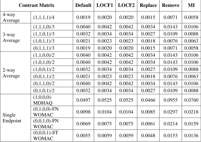
Assuming MCAR, missing responses can be handled with several approaches [24, 26]. Besides what has been provided above, one method manages missing values as tied with all other values in the same stratum. Another choice is the last observation carried forward (LOCF) based on the kernels of the U-statistics, or the observed value of 𝑌. Or, complete cases analyses is possible where patients with missing values are removed.
A R package that has all the features for the discussed approaches for the implementation of stratified multivariate Mann-Whitney estimators is readily available and straightforward to use [26]. 1.5 Handling Baseline Imbalance in Clinical Trials
15
The application of conventional parametric ANCOVA is through modeling, for example, linear regression model, logistic regression model, or Cox proportional hazard model, which relies on the statistical assumptions. In the settings of clinical trials, however, all analyses should have a priori specification in order to preserve the validity of the results, whereas the assumptions of the parametric ANCOVA are unverifiable. This dilemma led to the development of nonparametric randomization based ANCOVA for randomized clinical trials.
1.5.1 Nonparametric Randomization Based ANCOVA
Details for the methodology of nonparametric ANCOVA can be found in several published papers [28, 29]. Briefly, this approach is based on weighted least squares methods to analyze the differences between treatment groups while simultaneously restricting the differences in the covariates among treatment groups to be zero (i.e., correcting the imbalance). Specifically, let
𝒙𝒊𝒖= (𝑥𝑖𝑢1, … , 𝑥𝑖𝑢𝑚)′, denote the vector of 𝑀 covariables for the 𝑢th patient on treatment 𝑖. Then the sample mean of the response and sample mean of the covariables with respect to treatment 𝑖 are written as 𝑦̅𝑖 =𝑛1
𝑖∑ 𝑦𝑖𝑢 𝑛𝑖
𝑢=1 , and 𝑥̅𝑖 =𝑛1
𝑖∑ 𝑥𝑖𝑢 𝑛𝑖
𝑢=1 . Let 𝒇 = (𝑑𝑦, 𝒅𝒙′)′ where 𝑑𝑦= (𝑦̅1− 𝑦̅2), and 𝒅𝑥 = (𝒙̅1− 𝒙̅2). In this sense, 𝒇 is a vector that contains the differences in mean response and means for the covariates between the two groups. In a randomized trial, the expected value for 𝒅𝑥 would in fact be equal to zero. There are two ways to generate the covariance matrix for 𝒇. Under the null hypothesis of no treatment difference, the variance-covariance matrix 𝑽𝟎 is as follows:
𝑽𝟎= 𝑁
𝑛1𝑛2(𝑁 − 1)∑ [
(𝑦∗𝑗− 𝑦̅∗∗)2 (𝑦∗𝑗− 𝑦̅∗∗)(𝒙𝑗− 𝒙̅∗)′ (𝑦∗𝑗 − 𝑦̅∗∗)(𝒙𝑗− 𝒙̅∗)′ (𝒙𝑗− 𝒙̅∗)(𝒙𝑗− 𝒙̅∗)′ ] 𝑁
𝑗=1
Here 𝑦̅∗∗= ∑𝑛𝑗=1𝑦∗𝑗/𝑁 is the sample mean of the response variable for all patients in the trial under the null hypothesis, and 𝑦∗𝑗 is the response under the null hypothesis for patient 𝑗 regardless of treatment assignment. 𝒙̅∗= ∑𝑛𝑗=1𝒙𝑗/𝑁 is the sample mean vector for the covariables for all patients in the trial, and 𝒙𝑗 is the vector of covariables for patient 𝑗.
16 𝑽𝒔= ∑
1 𝑛𝑖(𝑛𝑖− 1) 2
𝑖=1
∑ [(𝑦 (𝑦𝑖𝑢− 𝑦̅𝑖)2 (𝑦𝑖𝑢− 𝑦̅𝑖)(𝒙𝑖𝑢− 𝒙̅𝒊)′ 𝑖𝑢− 𝑦̅𝑖)(𝒙𝑖𝑢− 𝒙̅𝒊)′ (𝒙𝑖𝑢− 𝒙̅𝒊)(𝒙𝑖𝑢− 𝒙̅𝒊)′] 𝑛𝑖
𝑢=1
This is under the assumption that the trial patients are a simple random sample from a very large population. 𝑽𝒔 allows population-based inference after covariance adjustment. 𝑽 can be further
partitioned as 𝑽 = [𝑽𝑽𝒚𝒚 𝑽𝒚𝒙′ 𝒚𝒙 𝑽𝒙𝒙].
A linear model 𝒇 = 𝒁𝑏 can be fit using the weighted least squares method to determine b, where 𝒁 = (𝟏 𝟎𝒑′)′, with 𝟎𝑝 denoting a (px1) vector of 0’s, and b represents the adjusted mean difference for the response. Determination of b can be obtained as (𝒁′𝑽−𝟏𝒁)−𝟏𝒁′𝑽−𝟏𝒇 = 𝑑𝑦− 𝑽𝒚𝒙′𝑽𝒙𝒙−𝟏𝑑𝑥 , where 𝑽 is either 𝑽𝟎 or 𝑽𝒔. An estimator of its covariance matrix is 𝑉𝑏 = (𝒁′𝑽−𝟏𝒁)−𝟏= 𝑽𝒚𝒚− 𝑽𝒚𝒙′𝑽𝒙𝒙−𝟏𝑽𝒚𝒙. This estimator is the exact variance of the randomization distribution of b when 𝑽𝟎is used; when 𝑽𝒔 is used instead, it corresponds to a consistent estimator of the variance of b.
When sample sizes are sufficiently large, i.e., 𝑛𝑖 ≥ 15√𝑀 + 1, 𝑄𝑏= 𝑏2/𝑉𝑏 has an approximate chi-square distribution with one degree of freedom. With 𝑉𝑏based on 𝑽𝒔 , a confidence interval for the mean difference of the response can be obtained. When sample sizes are not large, the assessment of b is possible through an exact p-value from the randomization distribution that uses 𝑽𝟎.
The main consideration for this method is that there is a valid randomization to the treatment groups so that the distributions of the covariables are statistically similar across the two treatment groups. 1.5.2 Stratified Studies and Multivariate Responses
The aforementioned nonparametric ANCOVA also has useful extensions for stratified studies [29, 30] and multivariate responses[29]. When independent randomization is conducted at a stratum level, analysis for the combined strata based on moderately large sample size (𝑛ℎ𝑖≥ 15√𝑀 + 1) is then
17
two treatments with adjustment for both covariables and strata. When the sample sizes are not large for all strata, covariance adjustment is applied after stratification adjustment rather than within each stratum. If multiple responses are to be analyzed based on a stratified design, the construction of the test statistic is 𝑄𝐴𝑏̅ = 𝑏̅′𝐴′{𝐴𝑉
𝑏̅𝐴′}−1𝐴𝑏̅, where A=𝟏′𝑟,denotes a (𝑟 × 1) vector of 1’s, 𝑏̅ and 𝑉𝑏̅ are calculated with modified 𝑍 = [𝐼𝑟, 0𝑟𝑃′]′, which has approximately the chi-square distribution with d.f.=1. For this version, 𝑄𝐴𝑏̅ is a stratified and covariance adjusted counterpart to the OLS method of O’Brien for multiple endpoints.
1.5.3 Dichotomous, Ordinal and Survival Outcomes
The nonparametric randomization based ANCOVA method can also have extensions to various types of response variables. For the dichotomous outcome, the sample mean of the responses for each treatment can be calculated as proportion 𝑝 and then transformed to 𝑙𝑜𝑔𝑖𝑡(𝑝) = 𝑙𝑜𝑔(1−𝑝𝑝 ) naturally. So the vector of differences 𝒇 can be created to include the differences in the log odds, which can be interpreted easily later as odds ratios, and the differences in the means of the covariables between two treatment groups. The weighted least squares method can then have application [29, 31]. When the outcome is ordinal, one approach is to expand the vector 𝒇 to accommodate the cumulative logits. Analysis can proceed as described previously with a multivariate extension of the covariance matrix. Alternatively, Mann-Whitney estimators with 𝒇 = (𝝃̂, 𝒅𝒙′) and the weighted least squares approach can be useful [24]. The transformation to the Logrank scores is applicable for the survival outcome for treatment 1 and 2 [31], or a hybrid method with the Cox proportional hazards model that only contains a treatment indicator can use the weighted least squares method with the log hazard ratio that compares treatment and placebo group as the response difference in the vector 𝒇. The subsequent statistics can be constructed in a similar way [23].
1.6 Innovative Applications
18
at multiple visits. While the main purpose for those trials normally is to prove the overall treatment efficacy, it is of particular interest to identify which of the endpoints are significant, or which of the visits carry the significant effect.
In this section, two examples are presented to illustrate the application of the multiway average closed testing procedure under those situations. The first example has four ordered categorical response variables at the four post-baseline visits, and they pertain to the comparison of two randomized treatments for a respiratory disorder. The second example discusses a randomized stroke clinical trial that has four efficacy outcomes for the comparison of a test treatment and placebo. The primary interest of the trial was to test the outcomes collectively to determine the overall treatment efficacy, then step down to see the efficacy of the individual outcomes.
1.6.1 Global Test
More generally, both 𝑇𝑂𝐿𝑆 and 𝑇𝑊𝐿𝑆 are applicable to a multivariate set of 𝑟 estimates 𝜷̂ for multiple comparisons between two treatments for multiple endpoints for one or more populations. For example, 𝜷̂ can be a set of estimates of mean differences between the test treatment and control group for a set of continuous endpoints. In this paradigm, when the underlying sample sizes are sufficiently large for 𝜷̂ to have an approximately multivariate normal distribution with asymptotic expected value 𝜀𝐴(𝜷̂) = 𝜷 and an essentially known covariance matrix 𝑽𝜷 through a consistent estimator 𝑽𝜷̂, then 𝑇𝑂𝐿𝑆=
(𝟏𝒓′𝜷̂) (𝟏⁄ 𝒓′𝑽𝜷̂𝟏𝒓)0.5 has an approximately normal distribution with expected value 0 and variance 1 under the global null hypothesis H0: β = 0. Similar considerations apply to
𝑇𝑊𝐿𝑆 = (𝟏𝒓′𝑽 𝜷̂
−𝟏𝜷̂) (𝟏 𝒓 ′𝑽
𝜷̂ −𝟏𝟏
𝒓) 0.5
⁄ . Also, if homogeneity applies to β in the sense that 𝛽 = 𝟏𝑟𝛿, then
𝑇𝑂𝐿𝑆 pertains to 𝜀𝐴(𝟏𝒓′𝜷̂) = 𝑟𝛿 and 𝑇𝑊𝐿𝑆 pertains to (𝟏𝒓′𝑽𝜷−𝟏̂ 𝟏𝒓) 𝛿 = 𝜀𝐴(𝟏𝒓′𝑽𝜷̂−𝟏𝜷̂).
1.6.2 Multiple Testing Strategy
19 𝑇𝑂𝐿𝑆= (𝑪′𝜷̂)/(𝑪′𝑽̂
𝜷𝑪)𝟏/𝟐 ~ 𝑁 (0, 1)
where 𝜷̂ is the vector of estimates for the comparisons, 𝑽𝜷̂is the estimated covariance matrix of 𝜷̂, and 𝑪 = 𝟏𝑟′.
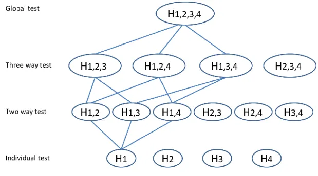
When the global test is rejected, a closed testing procedure is conducted to identify whether there is statistical significance in each of the subsets of endpoints through their OLS combined criterion, or the individual endpoints, at a predefined α level. As an illustration, if there is a set of 4 endpoints, 𝐻1, 𝐻2, 𝐻3, and 𝐻4 represent null hypotheses for the separate endpoints; and the closed family contains 15 hypotheses representing all possible intersections of 𝐻1, 𝐻2, 𝐻3, and 𝐻4. Each member of the closed family can be viewed as a global hypothesis and therefore can be tested using a global test with corresponding 𝑪. For example, when testing the hypothesis corresponding to the intersection of the first two comparisons, the contrast matrix will be 𝑪 = (1,1,0,0).
P-values for the hypothesis tests in this closed testing procedure are reported as multiplicity adjusted p-values. Specifically, results from a hypothesis and all of the other intersection hypotheses that imply this hypothesis are combined and the corresponding adjusted p-values are computed as the largest p-value among the p-values for the hypothesis and all the intersection hypotheses that imply it [15]. In this sense, if the adjusted p-value for an individual hypothesis test is less than the chosen significance level α, then the hypothesis is rejected.
1.6.3 Randomized Respiratory Disorder Trial with Four Visits
This example comes from a randomized clinical trial that compares a test treatment to placebo for a respiratory disorder. The listing of the data were published previously [6]. This trial had 111 patients from two centers, a baseline visit and four post-baseline visits that recorded patient global ratings of symptom control through a set of 5-category ordinal response variables as excellent, good, fair, poor and terrible. No missing values were observed in this example.
20
expected that the treatment effects are in the same direction for each of the post-baseline visits, evaluating the global effect as the average of several visits, and then stepping down to see the individual visits seems to be a reasonable approach.
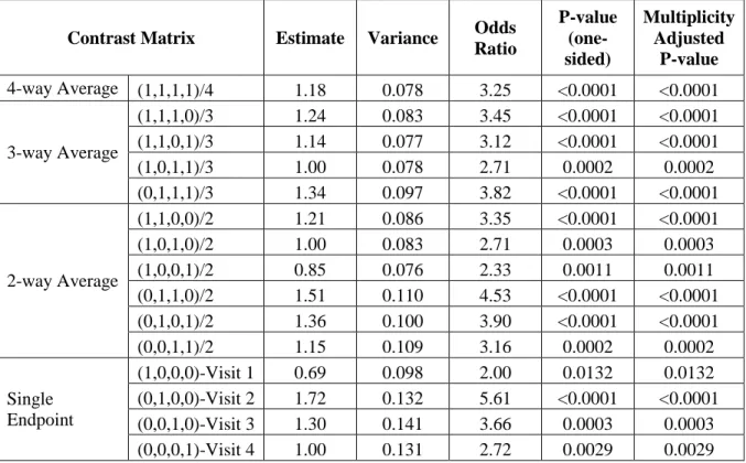
GEE for a proportional odds model was used to account for the four repeated measures of the global ratings of symptom control. The model included center, baseline ratings of symptom control, treatment group, visit, and treatment group by visit interaction as explanatory variables. Estimates for odds ratios for the treatment differences at each of the post-baseline visits and their covariance matrix were then provided by the model. For this case, the OLS global test shows p-value < 0.0001 (Table 1.1), which warrants the invocation of the subsequent closed testing procedure for the subsets of the OLS averages of the endpoints. Since all subsets of the tests, 3-way and 2-way averages, are significant, this strategy enables the validity of testing each of the single endpoints at a pre-specified one-sided α level 0.025 and preserves the FWER at this level in a strong sense.
Contrast Matrix Estimate Variance Odds Ratio P-value (one-sided) Multiplicity Adjusted P-value
4-way Average (1,1,1,1)/4 1.18 0.078 3.25 <0.0001 <0.0001
3-way Average
(1,1,1,0)/3 1.24 0.083 3.45 <0.0001 <0.0001
(1,1,0,1)/3 1.14 0.077 3.12 <0.0001 <0.0001
(1,0,1,1)/3 1.00 0.078 2.71 0.0002 0.0002
(0,1,1,1)/3 1.34 0.097 3.82 <0.0001 <0.0001
2-way Average
(1,1,0,0)/2 1.21 0.086 3.35 <0.0001 <0.0001
(1,0,1,0)/2 1.00 0.083 2.71 0.0003 0.0003
(1,0,0,1)/2 0.85 0.076 2.33 0.0011 0.0011
(0,1,1,0)/2 1.51 0.110 4.53 <0.0001 <0.0001
(0,1,0,1)/2 1.36 0.100 3.90 <0.0001 <0.0001
(0,0,1,1)/2 1.15 0.109 3.16 0.0002 0.0002
Single Endpoint
(1,0,0,0)-Visit 1 0.69 0.098 2.00 0.0132 0.0132
(0,1,0,0)-Visit 2 1.72 0.132 5.61 <0.0001 <0.0001
(0,0,1,0)-Visit 3 1.30 0.141 3.66 0.0003 0.0003
(0,0,0,1)-Visit 4 1.00 0.131 2.72 0.0029 0.0029
21
1.6.4 Randomized t-PA Stroke Trial with Multiple Outcomes
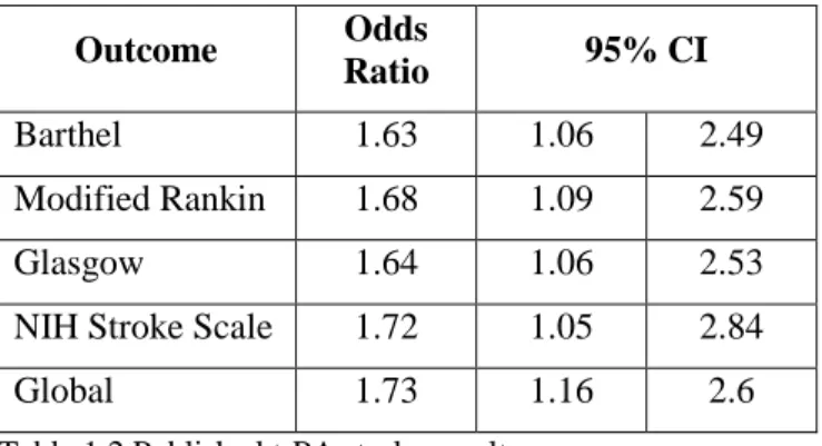
The National Institute of Neurological Disorders and Stroke (NINDS) has defined the treatment success of acute stroke as “consistent and persuasive difference” in the proportion of patients achieving favorable outcomes on the Barthel Index, Modified Rankin Scale, Glasgow Outcome Scale, and National Institutes of Health Stroke Scale. The consensus was: by categorizing outcomes as favorable /
unfavorable, outcomes are more clinically meaningful; a single outcome would not provide sufficient evidence of efficacy for stroke, thus a global test is appropriate [2]. Accordingly, the NINDS t-PA stroke trial was analyzed with a global test as the trial’s primary objective, and accompanied by secondary tests of individual outcomes (published results are quoted in Table 1.2). GEE was used to take the correlations among outcomes into account for the global test.
The reported strategy for controlling multiplicity in this t-PA stroke trial was to test the global hypothesis first at the α level 0.05; if statistical significance was observed, then testing proceeded to the four individual outcomes and with each outcome tested at α level 0.05. However, this strategy does not meet the strong control of FWER. Therefore, a re-analysis of the trial was performed based on the published results.
Because of the unavailability of patient level data, the covariance matrix for the GEE model β estimates was estimated in the following steps: assuming common correlation between each pair of the outcomes,
𝜌 = 16𝑉𝛽̅− ∑ 𝑉𝛽̂𝑖 4 𝑖=1 ∑ ∑4 √𝑉𝛽̂𝑖𝑉𝛽̂𝑗
𝑗=1 4
𝑖=1,𝑖≠𝑗
where 𝑉𝛽̂𝑖= (log (𝑂𝑅 𝑢𝑝𝑝𝑒𝑟/𝑙𝑜𝑤𝑒𝑟)1.96×2 )2 , 𝑖 = 1, 2, 3, 4, are the variances of the β estimates for the individual outcomes that can be computed from Table 2; 𝑉𝛽̅ is the variance of the β estimate for the global test. The
covariance for each outcome pair can then be computed as 𝑐𝑜𝑣(𝛽𝑖, 𝛽𝑗) = 𝜌 × √𝑉𝛽̂𝑖𝑉𝛽̂𝑗, where 𝑖 ≠ 𝑗. The
22
Outcome Odds
Ratio 95% CI
Barthel 1.63 1.06 2.49
Modified Rankin 1.68 1.09 2.59
Glasgow 1.64 1.06 2.53
NIH Stroke Scale 1.72 1.05 2.84
Global 1.73 1.16 2.6
Table 1.2 Published t-PA stroke results.
Since the global test for the OLS average met the required significance at one-sided 0.025 level (p-value=0.013), the closed testing procedure is performed for the subsets of the hypotheses, until the single endpoint level tests (Table 1.3). For this example, treatment efficacy applies for each of the single outcomes at the one-sided significance level 0.025.
Contrast Matrix Estimate Variance Odds
Ratio P-value (one-sided) Multiplicity Adjusted P-value
4-way Average (1,1,1,1)/4 0.51 0.053 1.67 0.0129 0.0129
3-way Average
(1,1,1,0)/3 0.50 0.051 1.65 0.0135 0.0135
(1,1,0,1)/3 0.52 0.054 1.68 0.0129 0.0129
(1,0,1,1)/3 0.51 0.054 1.66 0.0141 0.0141
(0,1,1,1)/3 0.52 0.054 1.68 0.0128 0.0129
2-way Average
(1,1,0,0)/2 0.50 0.052 1.65 0.0138 0.0138
(1,0,1,0)/2 0.49 0.052 1.64 0.0159 0.0159
(1,0,0,1)/2 0.52 0.056 1.67 0.0148 0.0148
(0,1,1,0)/2 0.51 0.053 1.66 0.0137 0.0137
(0,1,0,1)/2 0.53 0.056 1.70 0.0128 0.0129
(0,0,1,1)/2 0.52 0.057 1.68 0.0147 0.0147
Single Endpoint
(1,0,0,0)- Barthel 0.49 0.056 1.63 0.0191 0.0191
(0,1,0,0)- Modified Rankin 0.52 0.056 1.68 0.0144 0.0144
(0,0,1,0)- Glasgow 0.49 0.057 1.64 0.0188 0.0188
(0,0,0,1)- NIH Stroke Scale 0.54 0.065 1.72 0.0165 0.0165
Table 1.3 Re-analysis of the t-PA stroke trial
1.7 Summary of Research
23
Many confirmatory randomized clinical trials come with a stratified design. In addition, when the trial has random baseline imbalances, missing values, and strictly ordinal responses together with multiple endpoints, having an approach in place that can address multiplicity and solve other problems collectively and comprehensively is essential. A strategy is provided in Chapter 2 through a realistic case analysis. When two sources of multiplicity need to be managed simultaneously in one confirmatory clinical trial, the situation becomes complex and very challenging [32]. An example of such a situation is when the trial is focused on making primary inference on the overall population and/or some pre-specified subgroups, while multiple primary endpoints or key secondary endpoints are examined in each of the populations [4]. Chapter 3 proposes a strategy based on an innovative application of the closed testing procedure with multiway averages to address this complex multiplicity situation, and it applies this strategy to a real phase III confirmatory clinical trial. In addition, a simulation study is conducted based on this trial to compare the power of the proposed strategy to some more traditional alternative approaches.
When two or more sources of multiplicity exist in one confirmatory clinical trial, the control of the FWER is even more complex. For a clinical trial that is designed to have efficacy assessed with multiple primary endpoints, for multiple dose groups, and at two or more post baseline visits, the
objective is to have primary inference on all endpoints for at least one dose at any one of the visits. Under this situation, the prevailing multiplicity adjustment approaches through a fixed sequential testing
24
25 REFERENCES
1. Pincus, T., et al., An index of the three core data set patient questionnaire measures
distinguishes efficacy of active treatment from that of placebo as effectively as the American College of Rheumatology 20% response criteria (ACR20) or the Disease Activity Score (DAS) in a rheumatoid arthritis clinical trial. Arthritis Rheum, 2003. 48(3): p. 625-30.
2. Tilley, B.C., et al., Use of a global test for multiple outcomes in stroke trials with application to the National Institute of Neurological Disorders and Stroke t-PA Stroke Trial. Stroke, 1996.
27(11): p. 2136-42.
3. Sun, H., et al., Evaluating treatment efficacy by multiple end points in phase II acute heart failure clinical trials: analyzing data using a global method. Circ Heart Fail, 2012. 5(6): p. 742-9.
4. Morrow, D.A., et al., Vorapaxar in the secondary prevention of atherothrombotic events. N Engl J Med, 2012. 366(15): p. 1404-13.
5. Tangen, C.M. and G.G. Koch, Non-parametric analysis of covariance for confirmatory randomized clinical trials to evaluate dose-response relationships. Stat Med, 2001. 20(17-18): p. 2585-607. 6. Stokes, M.E., C.S. Davis, and G.G. Koch, Categorical Data Analysis Using SAS®. 2nd ed2000: SAS
Institute.
7. Marcus, R., P. Eric, and K.R. Gabriel, On closed testing procedures with special reference to ordered analysis of variance. Biometrika, 1976. 63(3): p. 655-660.
8. Holm, S., A Simple Sequentially Rejective Multiple Test Procedure. Scandinavian Journal of Statistics, 1979. 6(2): p. 65-70.
9. Hochberg, Y., A sharper Bonferroni procedure for multiple tests of significance. Biometrika, 1988.
75(4): p. 800-802.
10. Sarkar, S.K. and C.-K. Chang, The Simes Method for Multiple Hypothesis Testing with Positively Dependent Test Statistics. Journal of the American Statistical Association, 1997. 92(440): p. 1601-1608.
11. Lehmacher, W., G. Wassmer, and P. Reitmeir, Procedures for two-sample comparisons with multiple endpoints controlling the experimentwise error rate. Biometrics, 1991. 47(2): p. 511-21. 12. Troendle, J.F. and J.M. Legler, A comparison of one-sided methods to identify significant
individual outcomes in a multiple outcome setting: stepwise tests or global tests with closed testing. Statistics in Medicine, 1998. 17(11): p. 1245-1260.
13. Wright, S.P., Adjusted P-Values for Simultaneous Inference. Biometrics, 1992. 48(4): p. 1005-1013.
26
15. Dmitrienko, A., et al., Analysis of Clinical Trials Using SAS®: A Practical Guide2005: SAS Institute. 430.
16. O'Brien, P.C., Procedures for comparing samples with multiple endpoints. Biometrics, 1984.
40(4): p. 1079-87.
17. Pocock, S.J., N.L. Geller, and A.A. Tsiatis, The analysis of multiple endpoints in clinical trials. Biometrics, 1987. 43(3): p. 487-98.
18. Lefkopoulou, M., D. Moore, and L. Ryan, The Analysis of Multiple Correlated Binary Outcomes: Application to Rodent Teratology Experiments. Journal of the American Statistical Association, 1989. 84(407): p. 810-815.
19. Peto, R. and J. Peto, Asymptotically Efficient Rank Invariant Test Procedures. Journal of the Royal Statistical Society. Series A (General), 1972. 135(2): p. 185-207.
20. Koch, G.G., P.K. Sen, and I. Amara, Log-Rank Scores, Statistics, and Tests, in Encyclopedia of Statistical Sciences2004, John Wiley & Sons, Inc.
21. Wei, L.J., D.Y. Lin, and L. Weissfeld, Regression Analysis of Multivariate Incomplete Failure Time Data by Modeling Marginal Distributions. Journal of the American Statistical Association, 1989.
84(408): p. 1065-1073.
22. Saville, B.R., A.H. Herring, and G.G. Koch, A robust method for comparing two treatments in a confirmatory clinical trial via multivariate time-to-event methods that jointly incorporate information from longitudinal and time-to-event data. Stat Med, 2010. 29(1): p. 75-85. 23. Saville, B.R. and G.G. Koch, Estimating covariate-adjusted log hazard ratios in randomized
clinical trials using cox proportional hazards models and nonparametric randomization based analysis of covariance. J Biopharm Stat, 2013. 23(2): p. 477-90.
24. Kawaguchi, A., G.G. Koch, and X. Wang, Stratified Multivariate Mann–Whitney Estimators for the Comparison of Two Treatments with Randomization Based Covariance Adjustment. Statistics in Biopharmaceutical Research, 2011. 3(2): p. 217-231.
25. van Elteren, P.H., On the Combination of Independent Two-Sample Tests of Wilcoxon. Bulletin of the International Statistical Institute, 1960. 37: p. 351–361.
26. Kawaguchi, A. and G.G. Koch, sanon : An R Package for Stratified Analysis with Nonparametric Covariable Adjustment, 2014: The University of North Carolina at Chapel Hill Department of Biostatistics Technical Report Series.
27. Snedecor, G.W. and W.G. Cochran, Statistical Methods. 7th ed1980: Iowa State University Press. 28. Koch, G.G., et al., A review of some statistical methods for covariance analysis of categorical
27
29. Koch, G.G., et al., Issues for covariance analysis of dichotomous and ordered categorical data from randomized clinical trials and non-parametric strategies for addressing them. Stat Med, 1998. 17(15-16): p. 1863-92.
30. LaVange, L.M., T.A. Durham, and G.G. Koch, Randomization-based nonparametric methods for the analysis of multicentre trials. Stat Methods Med Res, 2005. 14(3): p. 281-301.
31. Tangen, C.M. and G.G. Koch, NONPARAMETRIC ANALYSIS OF COVARIANCE FOR HYPOTHESIS TESTING WITH LOGRANK AND WILCOXON SCORES AND SURVIVAL-RATE ESTIMATION IN A RANDOMIZED CLINICAL TRIAL. Journal of Biopharmaceutical Statistics, 1999. 9(2): p. 307-338. 32. Koch, G.G. and T.A. Schwartz, An overview of statistical planning to address subgroups in
28
CHAPTER 2: ANALYZING MULTIPLE ENDPOINTS
– an Approach that Addresses Stratification, Missing Values, Baseline Imbalance and Multiplicity for Strictly Ordinal Outcomes
2.1 Introduction
Multiplicity commonly arises in clinical trials when the effect of the test treatment is evaluated in multiple ways. For example, when no single endpoint describes all dimensions of the effect of the test treatment, multiple efficacy endpoints are present. The main concern for the multiplicity problem in the Phase III confirmatory clinical trial is that insufficiently controlled multiple assessments lead to multiple opportunities for the findings of a clinical trial to be due to chance. Without appropriate control, the trial loses its validity because of the inflation of Type I error. For the confirmatory clinical trial, strong control of family-wise (or the experiment-wise) Type I error rate (FWER) is typically necessary.
Besides multiplicity, the efficacy endpoints may also be strictly ordinal response variables, e.g. either ordered categories or continuous determinations that are not compatible with an interval scale. In addition, it is very common for confirmatory clinical trials to have a stratified design, for example, multicenter studies or according to baseline characteristics such as gender or disease severity, etc. Moreover, when comparing a test treatment to a control group, random baseline imbalances could occur. Also, missing values occur regardless how much effort has been involved in preventing them. When all those issues occur together in a single confirmatory clinical trial, controlling multiplicity while addressing all other issues simultaneously is not straightforward.
29
providing confidence intervals, having a multivariate extension to a set of 𝑟 outcomes, and handling possible missing data for one or more of the response variables assuming missing completely at random (MCAR) or other paradigms [1, 2]. In the case of potential concern for random baseline imbalance, nonparametric randomization-based covariance adjustment [3, 4] can have pre-specified invocation for the estimators by expanding the Mann-Whitney estimator vector to include the stratified differences between means of covariables, producing a consistent estimator of the corresponding covariance matrix and then constraining the differences for covariables to 0’s [1].
Closed testing through multiway averages can be a very useful approach in managing multiplicity [5], but it has been used less in the current clinical trial planning. It features a global test that addresses a global null hypothesis concerning treatment efficacy through a combination of endpoints, with the possibility for testing all possible subsets for combinations of endpoints, including the respective separate endpoints, if certain requirements are met. The whole process is under the strong control of FWER. For this paper, we illustrate combining stratified multivariate Mann-Whitney estimators for which randomization-based covariance adjustment is possible with the novel application of the closed testing procedure through multiway averages, and we develop an effective approach that is straightforward to implement and can additionally address missing data for some outcomes.
2.2 Methods
2.2.1 Stratified Multivariate Mann-Whitney Estimator
Let ℎ = 1, 2, … , 𝑞 index a set of strata within which patients have randomization to two treatment groups indexed by 𝑖 = 1, 2. Let 𝑘 = 1, 2, … , 𝑟 index the response variables, and 𝑗 = 1, 2, … , 𝑁 index the patients for the pooling of all patients regardless of their treatment group or strata. 𝑌𝑗𝑘 denotes the response for the 𝑗th patient with 𝑘th strictly ordinal response. Stratified multivariate
30
𝑖=2. 𝑍𝑗𝑘 indicates whether the response for 𝑗th subject and 𝑘th outcome is missing (set to 1 if it is not
missing, and 0 otherwise). Then 𝜃̂1𝑘 =𝑁(𝑁−1)1 ∑𝑁𝑗=1∑𝑁𝑗≠𝑗′𝑈1𝑗𝑗′𝑘, which pertains to the probability that a random pair of patients is from the same stratum and has a patient in group 1 with larger value for the 𝑘th response variable than the other patient in group 2, with tie breaks at probability 0.5;
𝜃̂2𝑘= 1
𝑁(𝑁−1)∑ ∑ 𝑈2𝑗𝑗′𝑘 𝑁
𝑗≠𝑗′ 𝑁
𝑗=1 , which pertains to the probability that a random pair of patients is from the same stratum and has non-missing values of the response for endpoint 𝑘 for both patients. In this construction,
𝑈1𝑗𝑗′𝑘 = 𝐼{(𝑆𝑗− 𝑆𝑗′) = 0} × [𝐼{(𝑡𝑗− 𝑡𝑗′)(𝑌𝑗𝑘− 𝑌𝑗′𝑘)𝑍𝑗𝑘𝑍𝑗′𝑘 > 0} + 0.5 × 𝐼 {(𝑡𝑗− 𝑡𝑗′)2𝑍𝑗𝑘𝑍𝑗′𝑘 >
0} × 𝐼{(𝑌𝑗𝑘− 𝑌𝑗′𝑘) = 0}] /(𝑛𝑗𝑘+ 𝑛𝑗′𝑘+ 1),
𝑈2𝑗𝑗′𝑘 = 𝐼{(𝑆𝑗− 𝑆𝑗′) = 0} × 𝐼 {(𝑡𝑗− 𝑡𝑗′)2𝑍𝑗𝑘𝑍𝑗′𝑘 > 0} /(𝑛𝑗𝑘+ 𝑛𝑗′𝑘+ 1).
𝐼(𝐴) has the value 1 if the condition 𝐴 is satisfied or the value 0 if otherwise, and 𝑌𝑗𝑘= 0 when 𝑍𝑗𝑘 = 0 without loss of generality; 𝑛𝑗𝑘 denote the sample size for the 𝑘th response variable for patients with the same stratum and treatment group as the 𝑗th patient.
A consistent estimator for the covariance matrix for 𝝃̂ is 𝑽𝝃̂= 𝑫𝝃̂[𝑫−1̂𝜽𝟏, −𝑫𝜽̂𝟐−1]𝑉𝑭̅[𝑫𝜽̂𝟏 −1, −𝑫
𝜽̂𝟐 −1]𝑫
𝝃̂, where𝑭𝑗= (𝑼𝟏′, 𝑼𝟐′)′, 𝑭̅ = (𝜽̂𝟏′, 𝜽̂𝟐′)′, and 𝑉𝑭̅=𝑁(𝑁−1)4 ∑𝑵𝒋=𝟏(𝑭𝒋− 𝑭̅)(𝑭𝒋− 𝑭̅)′.
31
When the sample size is large enough, e.g., 𝑛+𝑖𝑘 ≥ 50, and all 𝑛ℎ𝑖𝑘≥ 4, where 𝑛+𝑖𝑘= ∑𝑞ℎ=1𝑛ℎ𝑖𝑘, 𝝃̂ has an approximately multivariate normal distribution. Thus, the estimate of the overall treatment effect is 𝑪′𝝃̂, and the two-sided 100×(1-2α)% confidence interval for 𝑪′𝝃̂, with 𝑪′ = (𝑐1, 𝑐2, … , 𝑐𝑟) is 𝑪′𝝃̂ ± 𝑧𝛼√𝑪′𝑽𝝃̂𝑪, where 𝑧𝛼 is the 100×(1-α) percentile of the standard normal
distribution. For the average across all outcomes, 𝑪 = 𝟏𝑟/𝑟.
A R package called sanon that has all the features for the discussed approaches for the implementation of stratified multivariate Mann-Whitney estimators is readily available and straightforward to use[6].
2.2.2 Randomization Based Nonparametric Covariance Adjustment
Let 𝑚 = 1, 2, … , 𝑀 represent a set of 𝑀 numerical covariables that have observations (without missing data) prior to randomization. Let 𝑥ℎ𝑖𝑚𝑗 be the observed value of the 𝑚th covariable for the 𝑗th patient in 𝑖th treatment group of ℎth stratum. Let 𝑔𝑚 = (∑ℎ=1𝑞 𝑤̃ℎ(𝑥̅ℎ1𝑚− 𝑥̅ℎ2𝑚)/ ∑𝑞ℎ=1𝑤̃ℎ), with 𝑤̃ℎ= 𝑛ℎ1𝑛ℎ2/(𝑛ℎ1+ 𝑛ℎ2), and 𝑥̅ℎ1𝑚= ∑𝑛𝑗=1ℎ𝑖 𝑥ℎ𝑖𝑚𝑗/𝑛ℎ𝑖. Thus 𝑔𝑚 is the estimator from two-way
analysis of variance for the difference between the stratification adjusted means of the 𝑚th covariable for the two groups. Let 𝒇 = (𝝃̂′, 𝒈′)′, where 𝒈 = (𝑔1, 𝑔2, … , 𝑔𝑚). Since 𝒈 would be expected to be null on the basis of randomization of patients to the two groups, randomization-based covariance adjustment of 𝝃̂ is possible by fitting the model 𝑷 = [𝑰𝑟, 𝟎𝑟𝑀]′ to 𝒇 by weighted least squares. The resulting adjusted counterpart 𝒃 for 𝝃̂ is = (𝑷′𝑽𝒇−1𝑷)−1𝑷′𝑽𝒇−1𝒇 = (𝝃̂ − 𝑽𝝃̂𝒈𝑽𝒈−1𝒈) , where 𝑽𝝃̂𝒈 corresponds to the
covariance of 𝝃̂ with 𝒈 and 𝑽𝒈 corresponds to the covariance matrix of 𝒈. A consistent estimator for the covariance matrix of 𝒃 is 𝑽𝒃= (𝑷′𝑽𝒇−1𝑷)−1= 𝑽𝝃̂− 𝑽𝝃̂𝒈𝑽𝒈−1𝑽𝝃̂𝒈′.
2.2.3 Missing Values
32
Mann-Whitney estimators [1, 6] assuming MCAR or other paradigms. Besides the approach presented in Section 2.1, which manages missing values as missing and assumes MCAR, more settings are available in the sanon package. One method manages missing values as tied with all other values in the same stratum (in recognition that missing values cannot be classified as better or worse than observed values). Other specifications are the last observation carried forward (LOCF) based on the kernels of the U-statistic, or the observed value of 𝑌, or the complete cases analyses, in which patients with missing values are removed (and MCAR is assumed).
In addition, multiple imputations can have application when the assumption of MCAR is
questionable, with missing at random (MAR) being more reasonable. Specifically, assuming multivariate normal distributions, data are imputed through PROC MI with Markov chain Monte Carlo (MCMC) using SAS, with all the available response variables and covariates included in the imputation model, and 𝐿 datasets are generated during this step. SAS version 9.3 is used for the multiple imputations.
Mann-Whitney estimators 𝝃̂𝑖, and covariance structure for Mann-Whitney estimators 𝑾̂𝑖 are then computed for each of the imputed data sets using the R package sanon. Combining information from each of the imputations, one will have 𝝃̅ =1
𝐿∑ 𝝃̂𝑖 𝐿
𝑙=1 and 𝑽𝝃̅= 𝑾̅̅̅ + (𝐿+11 ) 𝑩 as the combined Mann-Whitney estimators and their estimated covariance structure, where ̅̅̅ =𝑾 1𝐿∑𝐿𝑙=1𝑾̂𝑖 and 𝑩 =𝐿−11 ∑𝐿𝑙=1(𝝃̂ −𝑖
𝝃̅)(𝝃̂ − 𝝃̅)𝑖 𝑇. Thus, the 95% confidence interval of 𝑪′𝝃̅ can be calculated as 𝑪′𝝃̅ ± 1.96 × √𝑪′𝑽𝝃̅𝑪. Such
methods are also applicable to the randomization-based covariance adjusted estimator 𝒃. 2.2.4 Global Test