Single-molecule force spectroscopy studies of fibrin A-a polymerization interactions via the atomic force microscope

(1)

Single-Molecule Force Spectroscopy Studies of Fibrin ‘A-a’ Polymerization Interactions via the Atomic Force Microscope

by Laurel E. Averett

A dissertation submitted to the faculty of the University of North Carolina at Chapel Hill in partial fulfillment of the requirements for the degree of Doctor of Philosophy in the

Department of Physics and Astronomy with Emphasis in Biophysics

Chapel Hill 2009

Approved by:

(2)

ABSTRACT

Laurel E. Averett: Single-Molecule Force Spectroscopy Studies of Fibrin ‘A–a’ Polymerization Interactions via the Atomic Force Microscope

(Under the direction of Professor Mark H. Schoenfisch)

(3)

(4)

ACKNOWLEDGEMENTS

This work would not have been possible without the help and support of a great number of people. My advisor, Professor Mark Schoenfisch, was critical to my growth as a scientist and researcher, and I appreciate the freedom, advice, and opportunities he has given me to find my way in science. I am indebted to Professor Oleg Gorkun for his help and guidance; this thesis would be a very different document without his aid. I thank Professor Boris Akhremitchev for his advice, collaboration, and valuable time. I am also grateful for all of the insightful conversations I’ve had the pleasure of participating in with the fibrinogen research group (including, among others, Professor Susan Lord, Professor Richard Superfine, Professor Mike Falvo, Professor Timothy O’Brien, Ricky Spero, and Nathan Hudson). I am also grateful for my training from Dr. Carri Geer, and the help of Kellie Beicker in conducting some of the solution condition experiments. Lastly, I’d like to thank Dr. Ryan Fuierer and the rest of the people at Asylum Research who helped me with every technical question I had, and were extremely generous with loaning us equipment and supplies.

(5)

every ignorant question of mine with endless patience. I am also constantly amused by the questions they think are only appropriate to ask a physicist. I have had the opportunity to work with many of the smartest, most driven, and funniest people I’ve known, and I’ll always be thankful for that.

(6)

List of Tables

Table 3.1. Summary of the force magnitude (F, in pN) and separation relative to event 2 (ΔS, in nm) (average ± standard deviation) for each

event in the characteristic pattern for every pair of fibrin(ogen) fragments and variants. Tip proteins were NDSK fragment unless otherwise noted. Substrate proteins are diluted 50% by mass with BSA unless otherwise noted. The number of curves with characteristic events, which are the only interactions subject to this

analysis, is included under the “n” column. 81

Table 3.2. Percentage of interactions that were characteristic (# characteristic

/ total # of curves with events * 100) 92

Table 4.1. Increases in contour lengths obtained with events 1 and 2 in parallel (Par) and series (Ser). Values represent averages of all curve types, weighted by the associated standard deviation. Errors represent the propagated standard deviation of each fitted parameter over n > 1000 force curves. Two values are given for populations that could not be fit with one Gaussian distribution

centered at a positive value. 116

Table 4.2. Kuhn lengths (in nm) obtained from fitting the force curves with the FJC model with events 1 and 2 in parallel (Par) and series (Ser). Values represent averages of all curve types, weighted by the associated standard deviation. Errors represent the propagated standard deviation of each fitted parameter over n > 1000 force

curves. 119

Table 4.3. Kinetic parameters for the forced dissociation of the ‘A–a’

interaction. 123

Table 6.1. Parameters of fibrin polymerization as a function of temperature

(12)

List of Figures

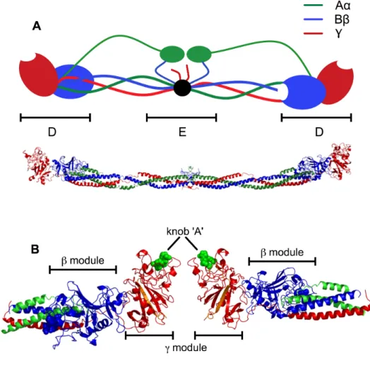
Figure 1.1. (A) Schematic (top) and crystal structure (bottom) of fibrinogen colored by chain. The D and E regions are indicated. In the schematic, the αC domains are shown interacting with the

N-termini of the Bβ chains. In the crystal structure, created using

Protein Data Bank entry 3GHG, neither the αC domains nor the

N-termini of the Aα and Bβ chains are resolved, and are therefore not

shown. (B) Ribbon depiction of two fibrinogen D fragments with bound knob ‘A’ and ‘B’ mimics, peptides GPRP and GHRP, respectively (spheres). C-terminal γ chain insert into β-sheet

colored orange. Constructed from Protein Data Bank entry 1LTJ. 3 Figure 1.2. Schematic of fibrin polymerization. (A) Fibrinogen monomer,

with both FpA and FpB in tact, and αC domains interacting with

FpB. (B) Thrombin cleaves FpA and FpB from the center of the molecule, exposing knobs ‘A’ and ‘B’. (C) Interactions between holes ‘a’ and knobs ‘A’ form double stranded, half-staggered protofibrils (αC domains and knobs ‘B’ not shown for C-E). (D)

Protofibrils grow and laterally aggregate to form fibers. (E) Fibers

grow, branch, and merge to form the complex fibrin network. 5

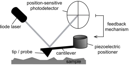
Figure 1.3. Schematic of the AFM. 10

Figure 1.4. Idealized force curve (A) and corresponding motions of the AFM probe (B). The tip approaches the substrate with zero deflection (1), making contact (2) and pressing into the substrate to a pre-determined set point (3). If a bond exists between the tip and substrate, the cantilever will deflect as it retracts (4) until the restoring force of the cantilever exceeds the strength of the bond,

which ruptures and the cantilever continues to retract (5). 11

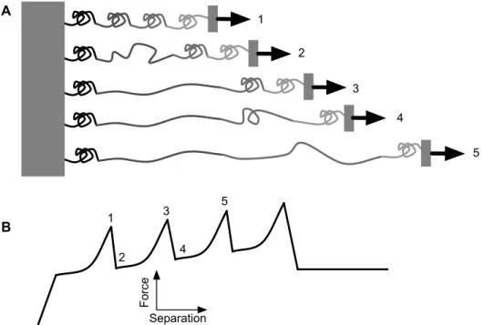
Figure 1.5. (A) Schematic of unfolding multi-domain proteins and (B) ‘saw tooth’ appearance of the associated force curve. Force applied to the multi-domain protein (1) ruptures a critical bond in one of the domains, allowing it to become unstructured (2). The ‘slack’ then extends in a manner well modeled as an ideal polymer (3) until the

critical bond in the next domain ruptures (4). 17 Figure 1.6. Schematic of energy landscape (with distance being the reaction

coordinate x) of a bond at equilibrium (left) and under force (right). The characteristic distance x‡, transition energy ΔG‡, and off-rate are indicated. Applied force F distorts the landscape in a distance-dependent manner so that the bound state is no longer the lowest

(13)

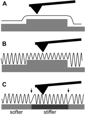
Figure 1.7. Schematic of (A) contact and (B, C) intermittent contact or tapping mode imaging with the AFM. In tapping mode, (B) changes in topology are represented by changes in the amplitude of the oscillation, (C) while changes in sample stiffness are represented by changes in the oscillation’s phase lag, indicated by

arrows. 27

Figure 2.1 Schematic of covalently immobilizing protein to a carboxylic

acid-terminated SAM through NHS/EDC chemistry. 60

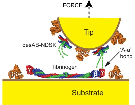
Figure 2.2 Schematic of AFM experimental configuration. Space-filling models of fibrin fragment desAB-NDSK and fibrinogen colored by polypeptide chains: α (green), β (blue), and γ (red). The formation

of ‘A–a’ bond is shown. The N-termini of the α chains do not

appear in crystal structures, therefore the knobs ‘A’ are approximated (dashed line). N-termini of β chains and αC domains

not shown. 62

Figure 3.1 Schematic representation of all proteins used in AFM measurements, not to scale. (A) Fibrinogen molecule depicted with

αC domains interacting with fibrinopeptide A and fibrinopeptide

B. Disulfide bond connecting the N terminus of the Aα chains

denoted as S-S. Locations of polymerization holes ‘A’ in γ module

and ‘B’ in β module indicated by arrows. (B) Fragments consisting

of the central part of fibrinogen (NDSK) and fibrin (desA- and desAB-NDSK) shown with both fibrinopeptides present (NDSK), FpA cleaved (desA-NDSK), and both fibrinopeptides cleaved (desAB-NDSK). (C) Polymerization holes-containing fragments D and DD. The location of DD interface containing interacting surfaces inaccessible to solvent is depicted by X in DD fragment. (D) Schematic representation of ‘A–a’ knob–hole interaction between desAB-NDSK (knob-containing molecule) and fibrinogen

(hole-containing molecule). 67

Figure 3.2 Force map showing interactions between 4A5 immobilized on the AFM tip and fibrinogen immobilized on the substrate in a 1 × 1

µm square with force curves taken every 31 nm. The black squares represent contacts resulting in an interaction while the white squares represent contacts without interaction. Interactions are defined as an abrupt change in force >5 standard deviations of the

baseline noise. 73

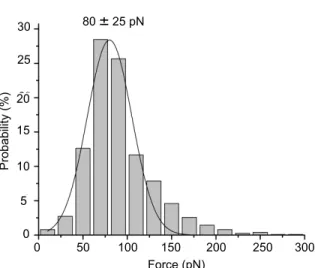
Figure 3.3 Distribution of observed forces between 4A5 and fibrinogen. Bin

(14)

Figure 3.4 Distribution of forces observed between desAB-NDSK immobilized on the AFM tip and fibrinogen immobilized on the substrate. The uncertainties represent widths at the

half-maximum of the Gaussian fits. Bin size = 20 pN. 75 Figure 3.5 Representative force curves showing prevalent patterns of rupture

of interactions between desAB-NDSK (tip) and fibrinogen (substrate). (A) Single event, (B) discarded force curve, and (C) four types of curves identified as the characteristic pattern of rupture. All characteristic curves include the doublet of events

above 200 pN. Event number is identified on each curve. 77 Figure 3.6 Plot of force versus separation relative to event 2 for all force

curves showing the characteristic pattern of rupture between

desAB-NDSK (tip) and fibrinogen (substrate). 78 Figure 3.7 (A) Distribution of forces (bin size = 20 pN) and (B) plot of force

versus separation relative to event 2 for characteristic interactions

between fibrin monomers on the tip and substrate. 80 Figure 3.8 Distribution of forces showing specificity of interactions between

tip and substrate modifications. Top: stepwise increase in number of interactions as fibrinogen knobs on each available surface are exposed. Bottom: interactions between desAB-NDSK and fibrinogen (left) are entirely inhibited upon incubation with GPRP (middle), and no interactions are found between desAB-NDSK and

γD364H (right). Each plot represents results from 3072

tip-substrate contacts. Bin size = 20 pN. 83

Figure 3.9 (top) Distribution of forces (bin size = 20 pN) and (bottom) plot of force versus separation relative to event 2 for characteristic interactions between (A) desAB-NDSK on the tip and fibrinogen nonspecifically adsorbed to the substrate, (B) desAB-NDSK on the tip and BβD432A fibrinogen on the substrate, (C) desA-NDSK on

the tip and fibrinogen on the substrate, (D) desAB-NDSK on the tip and D-fragment on the substrate, and (E) α chain on the tip and

fibrinogen on the substrate. 85

Figure 3.10 Force maps with contacts made every 156 nm along a 5 × 5 µm

area with desAB-NDSK on the tip and (A) 5%, (B) 10%, (C) 25%, and (D) 50% fibrinogen by mass in solution on the substrate. The black squares represent contacts resulting in an interaction, and the

white squares represent contacts without an interaction. 86 Figure 3.11 (A) Distribution of forces and (B) plot of force versus separation

(15)

between desAB-NDSK (tip) and the DD fragment (substrate). Note the histogram is not biphasic, but rather has a wide distribution of forces. The characteristic patterns seen with the DD fragment

exhibit events 1 and 4 less commonly than any other protein pair. 91 Figure 4.1 Force curves (restoring force in pN versus tip-substrate separation

in nm) containing characteristic pattern of fibrin ‘A–a’ knob–hole forced dissociation. Four types of characteristic patterns were identified: doublet (A), doublet with preceding event (B), doublet with following event (C), and doublet with both preceding and following events (D). Event numbers are indicated. Linear approximation of slope prior to one event as used for loading rate calculation is shown as dashed grey line (the line is slightly offset

for clarity). 103

Figure 4.2 Representative force curves not containing the characteristic pattern that were eliminated (A) automatically and (B) manually as described above. The automatic filter excludes curves with an overabundance of events (top), single events (middle), and curves that don’t fit the above definitions (bottom). The manual filter identified non-characteristic curves that passed the automatic filter but had events that were too far apart to be characteristic. These

often include a doublet of events. 107

Figure 4.3 (Left) Schematic of parallel, series, and zipper bond configurations. The force experienced by each interaction (F1

represents the first bond to rupture, while F2 represents the second

bond to rupture), relative to total applied force (F), is indicated. (Right) Hypothetical force curves for each configuration are illustrated. The total applied force (–), F1 (··) and F2 (--) are shown.

Select changes in restoring force in the force curves that correlate

with the changes in force applied to each bond are indicated. 111 Figure 4.4 Probability distributions of the rupture forces of a representative

experiment with tip retraction velocity of 1 µm/s and cantilever

stiffness of 55 pN/nm. 113

Figure 4.5 Representative four-event characteristic pattern force curve (circles) fit with the freely jointed chain model (lines). Least-squares fits with event 1 in parallel (grey) and in series (black) with event 2 are shown. Events 2–4 were always fit as in a series

configuration. 115

(16)

Bin size = 5 nm. Each row corresponds to a curve type: curves with events 2–3 (top row), curves with events 1–3 (second row), curves with events 2–4 (third row), and curves with all four events (last row). Since there were not large differences in the increase in contour length based on curve type, the values presented in Table 1 represent the averaged position and standard deviation of each fit for the increases in contour length after each event, weighted by the standard deviation. Since they aren’t characterized by an identifiable pattern, the initial contour lengths are omitted from

Table 4.1. 117

Figure 4.7 Probability distributions and Gaussian fits of Kuhn length for each event in each curve type as modeled with events 1 and 2 in (A) parallel and (B) series. Bin size = 0.05 nm. Each row corresponds to a curve type; the curve type corresponds to the events included in that row (e.g., the top row includes all curves that just exhibited events 2 and 3). Since there were no large differences in the values gained for each curve type, the values presented in Table 4.2 represent the averaged position and standard deviation of each fit for the Kuhn length of each event, weighted by the standard

deviation. 118

Figure 4.8 Characteristic force patterns of the rupture of interaction between fibrinogen and desAB-NDSK, where the rupture force is plotted versus (A) relative separation; relative contour length extracted from FJC fitted curves with events 1 and 2 modeled (B) in parallel

(C) in series or zipper. 120

Figure 4.9 Dissociation rates as a function of force for (A) each event as they occur in curves with just events 2 and 3 (), events 1–3 (), events 2–4 (*), and all four events () as identified in Figure 4.1, error bars represent error of the mean between experiments; and (B) each event with curve types averaged and weighted by error

(circles) and fit with Equation 4.3 (line). 121 Figure 4.10 Probability distributions and Gaussian fits of the elastic energy

stored the protein at time of rupture. The fit values for each event are — event 1: 130 ± 770 kBT; event 2: 1850 ± 1390 kBT; event 3:

2340 ± 1390 kBT; event 4: 970 ± 710 kBT. 126

Figure 5.1 Crystal structure of fibrinogen D fragment. GPRP (green spheres) and the γ1 calcium (orange sphere) are shown. Approximate

placement of β2 calcium is indicated. The following PDB entries

(17)

(DeLano Scientific, Palo Alto, CA). 134 Figure 5.2 Force versus separation aligned relative to the second event for

curves representative of each phenotype of the characteristic force curve. (Top to bottom) curves with just the doublet (events 2–3), curves with the doublet and a preceding event (events 1–3), curves with the doublet and a following event (events 2–4), and curves with all four events. Event numbers are indicated. Curves are aligned to event 2 to show consistent spacing between events, and

offset for clarity. Ticks on y-axis represent 100 pN. 137 Figure 5.3 Force versus separation relative to event 2 of all events in the

characteristic pattern of interactions between desAB-NDSK and fibrinogen in (A) HBS, (B) HBS + 3 mM CaCl2, (C) HBS + 1 mM

EDTA, (D) HBS + 1 mM EDTA + 2 mM CaCl2, (E) HBS + 0.1

mM EGTA, (F) HBS + 0.1 mM EGTA + 2 mM CaCl2, (G) HBS +

1 mM EDTA + 2 mM MgCl2, (H) HBS + 0.1 mM EgTA + 2 mM

MgCl2. Event numbers are indicated in (A). 139

Figure 5.4 Incidence of the characteristic pattern of fibrin ‘A-a’ bond rupture as a function of divalent ion concentration. Probability that an interaction was characteristic (i.e., contained the characteristic pattern, dark grey) and that a characteristic force curve contained event 4 (light grey) for interactions between desAB-NDSK and

fibrinogen in buffers with different divalent ion salt concentrations. 140 Figure 5.5 Characteristic pattern of forced rupture of fibrin ‘A-a’ interaction

with fibrinogen variants. Force versus relative separation for desAB-NDSK interacting with (A) γE132A fibrinogen, (B)

γD320A fibrinogen. 144

Figure 5.6 Normalized force probability distribution for (A) single event interactions between desAB-NDSK and wild-type fibrinogen, (B) single event interactions between desAB-NDSK and γD320A

fibrinogen, (C) events 3 (light grey) and 4 (dark grey) in characteristic interactions between desAB-NDSK and wild-type fibrinogen, and (D) event 3 in characteristic interactions between desAB-NDSK and γD320A fibrinogen. The center and standard

deviation of Gaussian fits (black lines) are indicated. The probability is normalized such that the area under the histogram

equals one. 146

Figure 6.1. Probability that (A) an interaction is characteristic and (B) a characteristic interaction includes event 4 as a function of NaCl concentration. The 0.15 M concentration represents the standard

(18)

Figure 6.2. Probability that (A) an interaction is characteristic and (B) a characteristic interaction includes event 4 as a function of pH. A pH 7.4 represents the standard operating conditions. Asterisks indicate statistical significance (i.e., p-value > 0.05) against the

standard conditions. 163

Figure 6.3. Probability that (A) an interaction is characteristic and (B) a characteristic interaction includes event 4 as a function of temperature. The temperature at 27 ºC represents the standard operating conditions. Asterisks indicate statistical significance (i.e.,

p-value > 0.05) against the standard conditions. 164

Figure 6.4. Absorbance at 350 nm as a function of time and temperature for fibrin polymerization. Fibrin polymerization was catalyzed by (A) thrombin and (B) batroxobin. The polymerization was investigated at three temperatures: 27 ºC (dashed line), 37 ºC (solid line), and

47 ºC (dotted line). 167

Figure 6.5. (A) Structure of γ module (ribbon) with bound GPRP peptide

(spheres). Location of all histidine residues in γ module are shown

with blue sticks. (B) Magnification of GPRP peptide (center) and residues in hole ‘a’ with which it has polar contacts (dashed lines). Note that the N-terminus of knob ‘A’ hydrogen-bonds with the His 340 (labeled). Created from PDB-ID 1LTJ using Pymol. (C)

Schematic of the protonation of histidine. 169

Figure 7.1 (A) Hypothetical force clamp separation versus time traces of fibrin ‘A-a’ knob-hole bonds. Inset is associated force ramp force versus separation trace. Each plateau represents a mechanically stable conformation associated with an event in the characteristic pattern (as indicated by color), and the rise between plateaus represents the increase in molecular length between the mechanically stable conformations. (B) Schematic of force quench experiment to examine protein refolding. Force is initially high, as in force clamp experiments (solid line), but is quenched to a much lower value (dotted line) and the separation is examined as a function of time. Integrity of refolded structure may then be tested

by a second unfolding cycle. 183

Figure 7.2 Schematics of unfold – refold cycles of three model biological systems. There is little to no hysteresis between the unfolding and refolding traces of myosin, an extracellular matrix protein comprised of α helix bundles. This lack of hysteresis suggests that

(19)

AFM. On the other extreme, the large hysteresis of the unfolding and refolding traces of multi-domain proteins like titin indicates that such proteins do not refold along the same energetic pathway they follow during unfolding. Schematics based on a figure from

(20)

List of Abbreviations and Symbols

~ approximately

° degree(s)

> greater than

< less than

% percentage(s)

# number

- negative

% percent

+ positive

± statistical margin of error

∞ infinity

αC C-terminus of the fibrin(ogen) α chain

β inverse thermal energy ∆ change

ΔG‡ transition energy

µg microgram(s)

µL microliter(s)

µm micrometer(s)

µM micromolar

µmol micromole(s)

(21)

τ bond lifetime

a persistence or Kuhn length

Å angstrom(s)

A350 absorbance at 350 nm

AFM atomic force microscope/microscopy

Ar argon gas

atm atmosphere

Au gold

BSA bovine serum albumin

C Centigrade

Ca2+ calcium ion

CaCl2 calcium chloride

CNBr cyanogen bromide

cm centimeter(s)

cos cosine

coth hyperbolic cosine

Cr chromium

desA without fibrinopeptide A

desAB without fibrinopeptides A and B

DNA dioxyribonucleic acid

E energy

EDC 1-ethyl-3-[3-dimethylaminopropyl]carbodiimide hydrochloride

(22)

e.g. for example

EGTA ethylene glycol tetraacetic acid

Eq. equation

et al. and others

EtOH ethanol

exp exponential function

F force

€

˙

F loading rate

Fc critical force

FJC freely-jointed chain

Fp fibrinopeptide

g gram(s)

G Gibb’s free energy

GHRP tetrapeptide glycine – histidine – arginine – proline (knob ‘B’ mimic)

GPRP tetrapeptide glycine – proline – arginine – proline (knob ‘A’ mimic)

h hour(s)

HBS HEPES-buffered saline

HBSC HEPES-buffered saline with calcium

HEPES hydroxyethyl piperazine sulfonic acid

HOPG highly-oriented pyrolytic graphite

ICP-OES inductively-coupled plasma optical emission spectroscopy

i.e. in essence

(23)

in inch(es)

k spring constant

kB Boltzmann’s constant

kBT thermal energy

koff off or dissociation rate

kon on or association rate

kDa kilodalton

kHz kilohertz

L contour length

L*(R) inverse Langevin equation

log logarithm

ln natural logarithm

m meter(s)

M molar

MΩ megaohm(s) min minute(s)

mg milligram(s)

Mg2+ magnesium ion

MgCl2 magnesium cloride

mL milliliter(s)

mm millimeter(s)

n number of samples

(24)

NaCl sodium chloride

NaF sodium fluoride

NaOAc sodium acetate

NDSK fibrin(ogen) N-terminal disulfide knot

NHS n-hydroxy succinimide

nm nanometer(s)

nmol nanomole(s)

nN nanonewton(s)

OM optical microscopy

OT optical tweezers

p probability

par parallel

PDB ID protein database identifier

PDMS polydimetyl siloxane

PEG polyethylene glycol

pH -log of proton concentration

pKa -log of acid dissociation constant

pmol picomole(s)

pN piconewton(s)

PU polyurethane

PVC polyvinylchloride

QCM quartz crystal microbalance

(25)

RMS root-mean-square

s second(s)

s-1 inverse second(s)

SAM self-assembled monolayer(s)

SEM scanning electron microscope/microscopy

ser series

sin sine

sinh hyperbolic sine

SMFS single-molecule force spectroscopy

SPR surface plasmon resonance

t time

T temperature

QCM quartz crystal microbalance

UV ultraviolet

V volt(s)

vmax maximum rate of change of A350

v/v ratio of volumes

vs. versus

WLC worm-like chain

× by

x distance

(26)

Chapter 1:

Introduction

1.1Fibrinogen and fibrin

Fibrin, the polymerized form of fibrinogen, the third most prevalent plasma protein, is

responsible for the structural stability of blood clots.1-6 Though the fibrin network

consists of only 0.25% of the volume of a clot, it is responsible for the structural integrity

of the clot under the flow of blood.7 Upon injury to a blood vessel, the coagulation

cascade generates thrombin, a serine protease, which converts soluble fibrinogen to

insoluble fibrin. Fibrin spontaneously polymerizes through non-covalent interactions and

forms a complex network of fibers that holds platelets, red blood cells, and other proteins

at the site of injury. Since fibrin is active in the flowing environment of blood, its

mechanical characteristics are critical for proper assembly, function, and eventual lysis.

Inappropriate mechanical properties of fibrin clots cause bleeding and clotting disorders

such as insufficient clotting and excessive bleeding (hemophilia), excessive clotting with

prolonged duration and vessel blockage (thrombosis), and dislodged clots that block

vessels away from the site of injury (thromboembolism). Furthermore, the biological

roles and physical properties of fibrin have made it an attractive biomaterial for tissue

(27)

1.1.1 Fibrin(ogen) structure. Fibrinogen, a 340 kDa protein, is a symmetric,

hexameric protein, consisting of three pairs of identical chains: the Aα, Bβ, and γ (Figure

1.1A).3, 5, 10-13 The N-termini of all six chains meet in the disulfide-rich central E region

of the molecule. The Aα and Bβ chains have disordered structures extending outwards

from the molecule with lengths of 27 and 64 peptides upstream of the first disulfide,

respectively. Each chain extends outwards in a coiled-coil towards the distal D regions.

The D regions contain the individually folded globule, largely homologous γ and β

modules. The γ module contains a high-affinity polymerization site known as hole ‘a’

with a critical calcium-stabilized loop, known as the γ1 calcium.14 The β module contains

a proposed polymerization site known as hole ‘b’, which also includes a

calcium-stabilized loop, β1.12 A second calcium binding site in the β module, β2, serves as a

bridge between the β and the coiled-coils, such that β module is held against the

coiled-coil with hole ‘b’ facing the center of the molecule.12 Both the modules comprising the D

region consist of mostly loops with short segments of coiled-coil, and a four-strand β

-sheet (Figure 1.2B). An unusual structural characteristic of the fibrinogen γ module is that

after forming the region around the hole, the C-terminus of the chain inserts into the

antiparallel β-sheet in its module, forming the second strand. Yakovlev et al. reported that

the γ module is functional (i.e., binds knob ‘A’) in the absence of this inserted strand.15 A

small interface is present between the γ and β modules that holds the γ module at a 30º

angle with respect to the coiled-coil. The C-terminus of the Aα chain folds back towards

the center of the molecule, interacting with the N-terminus of the Bβ chain.

To transform fibrinogen to active fibrin, thrombin cleaves fibrinopeptides A and B

(28)

Figure 1.1. (A) Schematic (top) and crystal structure (bottom) of fibrinogen colored by chain. The D and E regions are indicated. In the schematic, the αC domains are shown

interacting with the N-termini of the Bβ chains. In the crystal structure, created using

Protein Data Bank entry 3GHG, neither the αC domains nor the N-termini of the Aα and

Bβ chains are resolved, and are therefore not shown. (B) Ribbon depiction of two

fibrinogen D fragments with bound knob ‘A’ and ‘B’ mimics, peptides GPRP and GHRP, respectively (spheres). C-terminal γ chain insert into β-sheet colored orange. Constructed

(29)

them to the α and β chains and exposing polymerization sites known as knobs ‘A’ and

‘B’, respectively (Figure 1.2B).16 Thrombin preferentially cleaves FpA such that the

release of FpB is delayed in normal polymerization.17 The release of FpB frees the

fibrinogen αC domains from their interactions with the E region.18, 19 The ‘A’ and ‘B’

knobs noncovalently interact with preexisting polymerization sites, known as holes ‘a’

and ‘b’, in the γ and β modules, respectively, of other fibrin monomers (Figure 1.2C).16

Thus, half-staggered protofibrils are generated, and laterally aggregate to form fibers

(Figure 1.2D). The forces and interactions responsible for lateral aggregation are unclear,

but may involve ‘B-b’ knob-hole, αC–αC, and D–D interactions.3 The fibers grow,

branch, and fuse to form the complex fibrin network that serves as the structural scaffold

of a blood clot (Figure 1.2E). Finally, Factor XIII ligates the fibrin fibers in both the αC

and γ modules. Some controversy over whether γ ligation is longitudinal or lateral exists,

though for the purposes of the studies herein we will assume it longitudinal.4, 20-22

The difference between fibrinogen and fibrin is simply that fibrinogen retains the

N-terminal fibrinopeptides, FpA and FpB, which thrombin cleaves to transform fibrinogen

into fibrin. Due to the high affinity of knob ‘A’ for hole ‘a’, fibrin is rarely observed in its

monomeric form. Herein, the term fibrin(ogen) is used when either or both fibrin and

fibrinogen are meant. For example, the ‘A–a’ knob–hole interactions we study are

fibrin(ogen) interactions, since only fibrin has knob ‘A’, and fibrinogen is used as the

source of hole ‘a’.

1.1.2 Fibrin polymerization. Fibrin polymerization has mostly been characterized

(30)

Figure 1.2. Schematic of fibrin polymerization. (A) Fibrinogen monomer, with both FpA and FpB in tact, and αC domains interacting with FpB. (B) Thrombin cleaves FpA and

FpB from the center of the molecule, exposing knobs ‘A’ and ‘B’. (C) Interactions between holes ‘a’ and knobs ‘A’ form double stranded, half-staggered protofibrils (αC

domains and knobs ‘B’ not shown for C-E). (D) Protofibrils grow and laterally aggregate to form fibers. (E) Fibers grow, branch, and merge to form the complex fibrin network.

A

C

B

D

(31)

turbidity are the key parameters.21 Lag time is usually associated with FpA cleavage and

protofibril formation when the strands are not large enough to scatter light. Lateral

aggregation of protofibrils causes the turbidity to increase, so the rate of turbidity

increase is associated with the rate of polymerization. The final turbidity of the fibrin

network is proportional to the size of the fibers and the density of the network.23

Supplemental clot morphology characterization is often performed via scanning

electron or confocal microscopy.24 Final fibrin network structure is commonly reported in

terms of fiber thickness, pore size, and the number of branch points. The effects of the

concentrations of thrombin, fibrinogen, and calcium as well as pH, ionic strength, and

temperature on fibrin polymerization and structure have been studied previously, and will

be discussed in greater detail in Chapter 6.21, 24 While it may be intuitive to perform all

experiments in conditions that are physiologically relevant, the dynamic environment of

blood ensures that at least fibrinogen and thrombin concentrations are not static. To

understand fibrin polymerization in the diverse conditions of the vasculature, it is

necessary to examine fibrin in solution conditions over the physiologically relevant

range.

1.1.3 Fibrin mechanical properties. Since fibrin provides the structural support for

blood clots that must mitigate the shear forces of blood flow, it has an inherently

mechanical function. The straight appearance of fibers in fully polymerized fibrin

networks indicates that they are under strain even in static environments.6 The

mechanical properties of fibrin have been studied on multiple levels including the

(32)

structure under force. Viscoelastic and rheology studies of whole clots have focused on

the correlation between clot structure (i.e., thickness of fibers and porosity) and

mechanics.2, 25, 26 Other studies have examined the mechanics of fibrin fibers and

monomers. Individual fibers have been probed by both optical tweezers (OT)27 and

atomic force microscopy (AFM).28, 29 The use of the OT technique allowed individual

fibers to be manipulated in the context of a whole clot. Collet et al. reported that fibrin

fibers were relatively stiff compared to other biopolymers and exhibit strain-stiffening

behavior.27 The authors hypothesized that such behavior allows clots to both bend out of

the flow of blood, preventing vessel occlusion and resisting premature rupture. The AFM

experiments, where single fibrin fibers suspended over a polymeric microchannel were

mechanically extended, found that fibrin fibers are among the most extensible

biopolymers and that much of this extensibility is reversible.28-30

The discovery of the exceptional extensibility of fibrin fibers led to several

investigations into its source. At this juncture, two dominant hypotheses of the

mechanism responsible for fiber extensibility exist: protofibrils sliding with respect to

each other, and unfolding of structural domains within the monomers that comprise

protofibrils. These hypotheses are not mutually exclusive, and may each play a role in

fibrin extension at different strains. Falvo et al. reported that the extensibility of fibrin

fibers is correlated with the length of a natively disordered proline-rich section of the αC

region.29 Since there is evidence that lateral aggregation of protofibrils is at least partially

due to αC–αC interactions,6 this correlation points to protofibril sliding as the source of

fibrin extensibility. Others have used smaller fibrin oligomers to demonstrate that the

(33)

lends credence to intraprotofibril contributions to fibrin extensibility.31-33 Furthermore, a

recent study of the mechanical behavior of clots by small angle x-ray scattering suggests

that monomeric unfolding must occur in stretched fibers.33 In addition, the forced

unfolding of the γ module of fibrinogen may contribute to fibrin extensibility at high

strains.34, 35 It is unclear how each of these inter- and intraprotofibril mechanisms

contribute to the reversibility of fibrin fiber extension.

1.2Single molecule force spectroscopy

Recent technical advances in analytical tools commonly used to probe proteins such

as fluorescence resonance energy transfer, two-photon microscopy, electron microscopy,

molecular modeling, AFM, and OT, have enabled the examination of biological systems

at the single molecule level. By observing the behavior of single proteins (versus large

ensembles of biomolecules), previously ambiguous questions have been resolved. Due to

the advent of techniques that use force as the means to probe single molecule systems

(i.e., AFM36 and OT37), biophysics in particular has benefited from the expanding field of

single molecule force spectroscopy (SMFS). Force studies have shed light on mysteries

surrounding protein folding and structural stability.38 While both OT and AFM probe the

mechanical properties of single molecules, each has unique attributes that qualify it for

different applications. The OT technique typically has a low force regime capable of

measuring sub-piconewton forces with high temporal resolution, which make it

appropriate for force-clamp studies and examining many biological systems. However,

the spatial resolution of most OT systems prevents its use for examining protein folding.

(34)

range, has a lower-force limit of several piconewtons, restricting its use for some

biological systems. On the other hand, the sub-nanometer spatial resolution of the AFM

makes it the tool of choice for mechanical studies of protein folding and stability. Below,

the requirements for and typical applications of SMFS are outlined.

Despite the complexity of the data gathered, the AFM as a force sensor is both

requires only the most basic physical principles to describe, as shown in Figure 1.3 shows

and Figure 1.4 with a basic schematic and force curve, respectively. The AFM probe,

typically a silicon nitride pyramid, is affixed to the end of a micron-scale cantilever, and

moved towards and away from the substrate with sub-nanometer precision. The

cantilever’s deflections, detected with an optical lever comprised of a beam of light

reflected off of the back of the cantilever onto a position-sensitive photodetector, may be

translated into forces applied to the probe with Hooke’s law (i.e., F=-kx, where F is force,

x is deflection, and k is the empirically determined spring constant of the cantilever).36, 39

As the probe encounters the substrate, the cantilever is bent upwards until a

pre-determined deflection trigger is reached. The cantilever may then retracted from the

substrate at a constant velocity. If an interaction between the substrate and probe was

formed, the cantilever is bent downwards until the restoring force of the cantilever’s bend

exceeds the strength of the interaction, which breaks. The cantilever then continues to

retract at zero-deflection. The data collected from force spectroscopy experiments are

force versus separation traces, or ‘force curves’. The ‘strength’ of the interaction between

the tip and the substrate is the maximum force achieved, and the shape of the force curve

prior to rupture may be analyzed for clues about the behavior under force of the

(35)

Figure 1.3. Schematic of the AFM.

diode laser

piezoelectric positioner cantilever

tip / probe

position-sensitive photodetector

feedback mechanism

(36)

Figure 1.4. Idealized force curve (A) and corresponding motions of the AFM probe (B). The tip approaches the substrate with zero deflection (1), making contact (2) and pressing into the substrate to a pre-determined set point (3). If a bond exists between the tip and substrate, the cantilever will deflect as it retracts (4) until the restoring force of the cantilever exceeds the strength of the bond, which ruptures and the cantilever continues to retract (5).

1

2

3

4

5 1

2

3

4

5

A

B

force

(37)

Two primary goals exist for SMFS studies: forced unbinding of interactions between

molecules and forced unfolding of protein structures. For both aims, it is necessary to

take precautions to ensure that the phenomena observed are indeed single molecules, and

specific to the molecules of interest.

1.2.1 Experimental requirements for SMFS. Force spectroscopy may be, and often is,

performed on systems that are not single molecules. For example, the interactions of

bacterial cells with protein-coated substrates have been examined with the OT technique,

and correlations between binding forces and strain virulence found.40 Due to the

complexity of the force-separation traces, it is nearly impossible to draw anything but

qualitative conclusions from interactions between multiple pairs of molecules. In

addition, force spectroscopy is plagued by nonspecific interactions, which limits the

conclusions drawn from data. It is thus necessary to optimize methodology and perform

standard tests to ensure that the interactions measured are specific and between a single

pair of molecules.

The method of probe and substrate modification with proteins is a key element for

SMFS experiments. It is desirable to form a strong link between the protein and the

surface to reduce artifacts in the force data due to protein dislodging, while at the same

time preventing surface-related denaturation of the proteins so that the interactions of

interest remain intact throughout the experiment. The most common method for

immobilizing fibrinogen for force spectroscopy is nonspecific adsorption directly onto

the AFM probe. The primary drawback of this method is that adsorbed proteins are often

(38)

Since the interactions between the protein and the surface are not covalent, it is also

possible for the protein to become dislodged from the surface during the course of the

experiments, adding artifacts to the data. To account for these issues, crosslinkers

including glutaraldehyde, or self-assembled monolayers in combination with standard

NHS/EDC chemistry have been used to covalently attach fibrinogen to surfaces.41, 42

While polyethylene glycol (PEG) linkers for protein immobilization are more laborious

and costly, the known length and extension profile of PEG polymers facilitates data

analysis and filtering.43 Immunochemistry has also been used to immobilize proteins in

an oriented manner for probing the interactions between the substrate and specific sites

on the protein.44-46 To maximize the probability of single-molecule interactions, a

common strategy is to co-immobilize the protein of interest with a blocking protein such

as bovine serum albumin (BSA).47-49 Regardless of immobilization strategy, rinsing with

high-ionic strength and low-pH buffers is important to remove aggregates and loosely

adhered protein. Surfactants and excess blocking proteins have been included in the

buffers to reduce the likelihood of nonspecific interactions between the tip and

substrate.45, 49

To ensure that the interactions are specific, a series of controls involving

non-functional surfaces and interaction inhibitors are commonly performed.50-53 Since

nonspecific adhesion events often occur regardless of preventative measures, measures to

subtract the background that the nonspecific interactions cause have been taken.48, 54

Filters have also been employed to exclude low-force interactions at small tip-substrate

(39)

While there exist no standard procedures for ensuring the single-molecule nature of

interactions, a combination of several strategies have been employed to prove this

characteristic.38, 49 Since Poisson statistics indicate that an interaction frequency of

roughly 10–20% implies that the majority of interactions are between single molecules,

protein immobilization procedure is often optimized so that the interaction probability is

in this range.55 In addition, a method to check the single-molecule nature of interactions

has been utilized whereby the relationship between concentration of protein immobilized

and both the frequency and magnitude is determined.48, 56 If the interactions are between

single pairs of molecules, the frequency of the interaction should vary directly with

surface coverage, while the force magnitude should remain constant. A last method to

identify single-molecule interactions has involved examining the shape of the force

probability distributions. Single-molecule interactions should both result in a

characteristic shape with a long low-force tail and drop off quickly at high forces, while a

high-force tail is indicative of interactions between multiple molecules.51

1.2.2 Interactions between molecules. While interactions between single pairs of

molecules have been studied with the AFM since the inception of force spectroscopy, the

difficulties associated with the methodology required to eliminate non-specific

interactions and interactions between multiple pairs of molecules has limited the

conclusions drawn from such experiments. Reviews of the breadth of these experiments

can be found elsewhere,38, 49, 57 and only a few notable cases will be described below.

Perhaps unsurprisingly, the first and most widely characterized model system of

(40)

experiments by Lee et al. used BSA to covalently link biotin to a microsphere

immobilized on the AFM probe, and streptavidin to a mica substrate, detecting unbinding

forces of ~350 pN.58 Since then the multiple-valence nature, strength, and ubiquity of the

streptavidin–biotin interaction has made it an attractive target for more recent

examination of force-mapping,59 the effects of multiple parallel bonds in force

spectroscopy,51 and association kinetics.53 Other biological interactions commonly

examined with the AFM include protein–receptor,60-62 antibody–antigen,41, 46, 63 and

peptide–DNA.64

One particularly interesting class of interactions recently investigated with SMFS is

catch bonds.65 Discovered in studies of the flow-rate dependence of bacterial adhesion to

protein-coated surfaces, catch bonds become stronger when force is applied. Among the

protein systems that have demonstrated catch bond behavior are interactions responsible

for Escherichia coli binding to red blood cells, interactions involved in cellular motion,

and interactions critical to leukocyte adhesion to blood vessel walls.66 Such bonds have

been identified using two methods for plotting the force data: off-rate versus force, and

force versus loading rate. In plots of bond off-rate versus applied force for catch bonds,

the off-rate decreases with increased force (a situation opposite to normal interactions). If

the data is instead plotted as bond strength versus loading rate, catch bonds will exhibit a

dramatic increase in bond strength above some critical loading rate, as opposed to

monotonically increasing bond strength seen for other bonds.61, 67

1.2.3 Forced unfolding of protein structure. Studies of protein (un)folding and

(41)

The breadth of such studies may be found in thorough reviews elsewhere.38, 68-71 In 1997,

Rief et al. discovered that the multidomain-repeat muscle protein titin could be unfolded

with the AFM.72 In these experiments, titin was nonspecifically adsorbed to mica, and

force curves were acquired with nonfunctionalized probes. The resulting force curves

exhibited a characteristic sawtooth appearance, with the peak of each ‘tooth’ representing

the rupture of a critical bond that allowed the extension of an unstructured domain,

represented by the drop and following rise in force (Figure 1.5). The sawtooth curves

have been fit with ideal polymer models to extract information regarding the length of the

fully unfolded peptide chain, as well as its remaining structure, as is described below.50,

71, 73, 74_{Since these seminal experiments, the behavior of titin under force has been}

characterized by several groups.75 Recombinant titin variants have been constructed to

examine the effect of calcium ions on mechanics,76 engineer differences in mechanical

strength,77 and create disulfides.78 Titin has been used as a model protein system to

demonstrate molecular dynamics simulation of AFM techniques,79 force clamp

methodology,80 and examine the importance of pulling direction in forced unfolding of

proteins81 and protein refolding under tension.82

The extension of other proteins has also been initiated using AFM. Myosin, a long

double-stranded coiled-coil structure has been probed and found to be an elastic structure

with no hysteresis between the folding and unfolding force traces.83 In contrast, each of

the short double-stranded coiled-coil domains of spectrin has been shown to

cooperatively unfold.84 Other multi-domain repeat proteins such as fibronectin have

proven to have similar mechanics to titin.81, 85 Likewise, other engineered proteins

(42)

Figure 1.5. (A) Schematic of unfolding multi-domain proteins and (B) ‘saw tooth’ appearance of the associated force curve. Force applied to the multi-domain protein (1) ruptures a critical bond in one of the domains, allowing it to become unstructured (2). The ‘slack’ then extends in a manner well modeled as an ideal polymer (3) until the critical bond in the next domain ruptures (4).

5

Force

Separation

1

2

3

4

1

2 3

4 5 A

(43)

been mechanically probed. Each of these studies has provided insight into the mechanics

and stability of protein structure and the mechanisms involved in protein folding.

1.3Single molecule force spectroscopy analysis

Several types of information have been gained from SMFS studies by careful analysis

of the information acquired. First, the elasticity of the tether (i.e., the mechanical

properties of the intact molecular construct) has been examined by analyzing the force

curve prior to final bond rupture.38, 90 In addition, kinetic parameters such as the rates of

bond association and dissociation have been deciphered.57, 61, 70, 91 The association rate

(i.e., on-rate) dictates how quickly a bond is formed, and is commonly limited only by the

rate of diffusion of the molecules associated with the bond, though structural changes or

other energetic barriers to bond formation slow the association rate.53 The dissociation

rate (i.e., off-rate) depends on the depth of the energy well of the bound species, and is

the inverse of the half-life of the bond. These parameters have provided insight about the

relationship of the mechanical energy landscape to that of thermal or chemical

denaturation and bond rupture.74, 92, 93

1.3.1 Polymer-like behavior. Force spectroscopy experiments have traditionally been

designed to examine forced unfolding of proteins. This is exceptionally useful to study

mechanical proteins comprised of multiple, identical domains, including titin,72, 76, 94

chromatin,95 myosin,83 spectrin,84 fibronectin.94, 96 and nebulin.97 Unfolding these proteins

is characterized by a saw-tooth pattern in the force curve, with each ‘tooth’ representing

(44)

To best understand the unfolding structures, the unraveling portions of the curve may be

fit with models describing an ideal polymer chain.73 These polymer chain models,

notably the worm-like chain (WLC) and freely jointed chain (FJC), use two parameters:

the contour length (i.e., end-to-end distance of a fully extended chain), and a shorter

length describing the stiffness of the chain (i.e., the persistence or Kuhn length for the

WLC or FJC, respectively).98 With the aid of these parameters, the unfolding structures

may be estimated. The most common information sought is the increase in contour

length, ΔL, between ruptures, which elucidates the structural regions unfolded.

The earliest and most commonly used model is the WLC model for its analytical

simplicity.72 A WLC is a homogeneous chain that may bend with a limited radius of

curvature, much like a garden hose without kinks. These chains are characterized by their

persistence length, which is the minimum distance between monomers required to

eliminate communication between the monomers.98 In other words, if the orientation of

one monomer is perturbed, monomers over a persistence length away will not be affected

by the perturbation. The longer the persistence length, the less stiff the polymer (i.e., the

polymer may be extended such that its end-to-end length nears its contour length with a

minimum application of force). For unfolding proteins, persistence lengths ~0.4 nm, the

approximate size of a single amino acid, are common.69 The relationship between force F

and end-to-end length x of such a chain is:

€

F = kBT

a

1

4 1

(

−x_L

)

2 −1 4+ x L          

, (1.1)

(45)

Methods have been developed to employ the FJC model for unfolding proteins.73, 99

An FJC is a chain of rigid, volumeless monomers that may flex in any direction at their

joints. The Kuhn length, is similar to the persistence length in that it describes the

minimum unit of length of the FJC that acts as an ideal polymer. However, polymers

described as an FJC will have a Kuhn length approximately twice the persistence length

of the same polymer described as a WLC.73 The relationship between force and the

end-to-end length of a FJC is:

€

F = kBT a

(

)

L*₍_R₎_, _(1.2)

where a is the Kuhn length, kBT is the thermal energy, R is the extension ratio (end-to-end

distance / contour length), and L*(R) = y is the inverse Langevin function, where L(y) =

coth(y)-1/y. Since the inverse Langevin function is not an analytic function, several

approximations have been developed to approximate the FJC at different extension ratios.

Most recently, a simple closed-form function L*(R) = (1-R)-1+(1-R)2, has been used to

great success.53

Despite the success of these models, caution must be used in applying either of them

to a real system such as protein unfolding.73 Since they are both ideal polymers, by

definition they ignore interactions between monomers. This is an especially egregious

mistake when modeling proteins that are comprised of monomers capable of

experiencing hydrophobic effects, hydrogen bonding, electrostatic interactions, and steric

hindrance. Information gained from using these models may thus be inaccurate in several

ways. Nevertheless, as a first approximation, the WLC and FJC are adequate for most

(46)

1.3.2 Kinetic Parameters. In 1997, Evans and Ritchie developed a method of gaining

kinetic information from single molecule force spectroscopy experiments based on an

earlier paper by Bell100 (appropriately called the Bell-Evans model).101 This model

suggests that the force of rupture is dependent on the loading rate (i.e., rate at which the

force applied to a bond increases) in a manner determined by the off rate at zero applied

force and the characteristic distance (i.e., distance between bound and transition states).

The equation defining this dependence is

€

F = kBT

x ln ˙ F x k_off

_{( )}

0 k_BT



 





, (1.3)

where x‡ is the characteristic distance, koff(0) is the zero-force off rate, and

€

˙

F is the

loading rate (Figure 1.6). Of note, this model assumes that both the zero-force off rate

and characteristic distance are loading rate-invariant. By finding the force at which the

bond ruptures under a range of loading rates (usually varied by changing the probe retract

velocity), these kinetic parameters may be obtained. This simple model has been

successfully applied to many systems within experimental error.70 Furthermore, studies

have reported the results of such analysis to be close to the corresponding kinetic

parameters gained from traditional equilibrium biochemical assays.

Significant attention has been given to the non-linear behavior of force versus loading

rate. Deviations from linear behavior have been attributed to multiple barriers between

the bound and unbound state.102, 103 Using the Bell-Evans formalism, complexity in the

energetic landscape correlates with a change in slope of the force-loading rate curve at

high loading rates.104 Akhremitchev and colleagues have demonstrated that such changes

(47)

Figure 1.6. Schematic of energy landscape (with distance being the reaction coordinate

x) of a bond at equilibrium (left) and under force (right). The characteristic distance x‡_,

transition energy ΔG‡, and off-rate are indicated. Applied force F distorts the landscape

(48)

Others have explained non-linearity in trends of F versus ln(

€

˙

F ) by accounting for

assumptions made in the Bell-Evans model.105 For example, models have been used to

include possible changes in the characteristic distance with loading rate. Schlierf and Rief

included a term in the most-probable force function explicitly describing the shape of the

energy well (in an experiment using the immunoglobulin-like domain ddFLN4, the

energy well was found to be funnel-shaped).105 However, execution of this model is

difficult and is highly dependent on the shape of the well. Dudko, Hummer, and Szabo

have developed a more robust method of modeling forced unbinding experiments using

only two additional variables that describe the shape of the well: ΔG‡ and ν, the energy

difference between bound and transition states and a term giving the approximate shape

of the well, respectively.93 Their method suggests transforming the data into off-rate as a

function of force (see below), and then fitting the trend with

€

k_off(F)=k_off(0) 1−νFx ΔG       1

ν−1

exp ΔG1− 1−νFx ΔG       1 ν                 

, (1.4)

where the most common values of _ν are 2/3 and 1/2, corresponding to the linear-cubic

and cusp shapes of the energy wells. In the case of ν = 1, this model reduces to the

Bell-Evans approximation. One drawback of this technique is that it is only applicable below

the critical force (Fc = ΔG‡/νx‡), above which the barrier disappears. As this is an artifact

of the model, other models may be used at high forces to extend the

Dudko-Hummer-Szabo model past this limit.

It may be desirable to use the off-rate as a function of force trend rather than force as

a function of loading rate since loading rates may vary considerably within and between

(49)

constant of the probe and the compliance of the tether. Further, this transformation allows

velocity-clamp experiments to be directly compared to force-clamp experiments, in

which the lifetime of a bond (τ = 1/koff) is investigated as a function of force. To perform

the transformation from (F) to koff(F), the relationship

€

k_off(F)= p(F) ˙ F (F)

p(F')dF' F

∞

∫

(1.5)

is used. The trends for several different experiments at different loading rates may be

averaged to sample a wider range of forces than would be accessible with a single

loading rate.

The kinetic parameters extracted from force spectroscopy techniques have been

compared to those obtained from other techniques (i.e., chemical and thermal

denaturation).74, 92, 93 In particular, the zero-force off-rate may be investigated via surface

plasmon resonance and other non-equilibrium techniques.106 The free energy difference

between the bound and free states, as established by the Hummer-Dudko-Szabo model,

have been compared to results from techniques such as isothermal calorimetry.57 Indeed,

several studies have compared the energy landscapes of a few model systems as

investigated by both force spectroscopy and other techniques.107 Such comparisons have

revealed that the reaction coordinate dictates the agreement between techniques, as the

pulling direction affects the kinetic parameters of proteins unfolded by force.81, 108 Some

directions are ‘good’ parameters for unfolding or unbinding studies, as they closely

mimic thermal denaturation or unbinding.

1.4 Fibrin(ogen) and the AFM

!

Single-molecule force spectroscopy studies of fibrin A-a polymerization interactions via the atomic force microscope

Table of Contents

List of Tables

A

C

B

D

A

B

(

)

(

)

( )

∫

_{( )}