Temporal-spatial modeling for fMRI data

(1)

Temporal-Spatial Modeling for fMRI Data

Ping Bai

A dissertation submitted to the faculty of the University of North Carolina at Chapel Hill in partial fulfillment of the requirements for the degree of Doctor of Philosophy in the Department of Statistics and Operations Research.

Chapel Hill 2007

Approved by

Advisor: Dr. Young Truong

Co-Advisor: Dr. Richard L. Smith

Reader: Dr. Haipeng Shen

(2)

(3)

ABSTRACT

PING BAI: Temporal-Spatial Modeling for fMRI Data (Under the direction of Dr. Young Truong)

By generating high quality “movies” of the brain in action, functional Magnetic

Res-onance Imaging (fMRI) helps us examine which parts of the human brains are activated

by different task performances. Many techniques for fMRI analysis have been developed

in the last decade. Independent component analysis (ICA) is an effective data-driven

method to explore spatio-temporal features in fMRI data. It has been especially

success-ful to recover brain-function-related signals from recorded mixtures of unrelated signals.

Due to the high sensitivity of MR scanners, spikes are commonly observed in fMRI data

sets and they deteriorate the analysis. No particular method exists yet to address this

problem. In the first part of this work, we introduce a supervised singular value

decompo-sition technique into the data reduction step of ICA. The proposed method improves the

robustness of ICA against spikes and makes the computation more efficient by using the

particular fMRI experiment designs to guide the fully data-driven ICA. The advantages

are demonstrated using a simulation study as well as a real data analysis.

ICA aims to separate blind source signals from their linear mixture signals based on

the assumptions of the statistical independence and non-Gaussian distributions of the

source signals. The second part of this work studies the methodology of some most

popular ICA algorithms and propose to evaluate some of the algorithms by assessing

the variability of the estimates of the mixing matrix through a nonparametric bootstrap

procedure. Two maximum likelihood ICA algorithms are studied in detail through a

simulation study.

(4)

model-driven strategies. Among them, the most widely used approach is statistical parametric

mapping (SPM), where the key technique is general linear model (GLM) and the

tem-poral characteristic of the expected response is usually modeled by the convolution of

the experiment stimulus and a predefined hemodynamic response function (HRF).

How-ever, the subjective assumptions of the form of HRF introduce estimation biases and

subsequently reduce the detection power of activation. In the third part of this work,

we propose a new nonparametric method to model the time component adaptively in

the context of SPM. The idea is to start from an initial time component obtained from

general SPM procedure and then apply a penalized smoothing technique to update the

shape of the hemodynamic response in an adaptive way. The nice performance of the

proposed method is illustrated through a simulation study as well as a real fMRI data

analysis.

Event-related fMRI (ER-fMRI) has played an important role in many recent brain

imaging studies to explore the relationship between recorded fMRI signals and neural

activity. Different from traditional block-design fMRI, ER-fMRI is very good at

estimat-ing the timestimat-ing and waveform of the hemodynamic response. Various methods have been

proposed in the literature to model the HRF. However, most of them have a number of

limitations. In the last part of this work, we propose a novel regression approach to

es-timate the HRF directly. The approach is based on point processes modeling to account

for the event-related designs. Compared to the existing methods, the proposed procedure

yields simultaneously the nonparametric estimate of the HRF and a test for the linearity

assumption. To illustrate its usefulness and the scientific implications, we applied this

procedure to study the spatial variation of the HRF, and the extent to which the linear

relationship holds in various regions of interest for Parkinson’s disease patients.

(5)

ACKNOWLEDGMENTS

The writing of this dissertation has been one of the most significant academic

chal-lenges I have ever had. I owe my deepest gratitude to all those people who have made

this dissertation possible and because of whom my graduate study in the past five years

has been a most enjoyable, rewarding and unforgettable journey in my life.

First of all, I would like to gratefully and sincerely thank my advisor, Dr. Young

Truong, for his guidance, patience and most importantly, his friendship during my

grad-uate study at UNC. I have always been feeling fortunate to have an advisor who not only

guided me in the wonderful research world, but also taught me the philosophy of life in

the real world. I deeply appreciate his confidence and belief in me. Through out my

graduate work, he continually stimulated my analytical thinking and greatly assisted me

with scientific writing.

A special thanks goes to Dr. Haipeng Shen, who has been a friend and mentor. He

taught me how to write academic papers and brought out the good ideas in me. He was

always there to meet and talk about my ideas, to proofread and mark up my papers, and

to ask me good questions to help me think through my problems.

I am grateful to Dr. Xuemei Huang for her encouragement, patience and all the

thought-provocative discussion. I am also thankful to her for allowing me to use the

computing facilities in her lab, reading my papers, commenting on my views and helping

me better understand my research from the point of view of a neurologist. I am also

indebted to the members of Dr. Huang’s fMRI lab with whom I have worked during the

(6)

Lewis and Dr. Suman Sen for the many valuable discussions that helped me understand

my research area better. My sincere thanks to Cara Slagle, Andrew Smith and Roxanne

Poole for their patience and all the data-related assistance whenever I needed.

I would like to acknowledge Dr. Richard Smith, who reviewed my work and gave

insightful comments, and Dr. Chuanshu Ji, who has given his time to read this manuscript

and gave me guidance in the early stages of my graduate study.

Many friends have helped me a lot through these years. Their support and care

helped me overcome setbacks and stay focused on my graduate study. I greatly value

and appreciate their friendship.

Finally, and most importantly, I would like to express my heart-felt gratitude to my

family, who has been a constant source of love, concern, support and strength all these

years. I thank my parents for educating me to be what I am, for unconditional support

and belief in me no matter what. Also, I thank my two sisters, the greatest in the world,

for sharing their experience of the graduate study endeavor with me, for listening to my

complaints and frustrations, and for always believing in me.

Part of this research is supported by NSF DMS-0707090.

(7)

LIST OF FIGURES

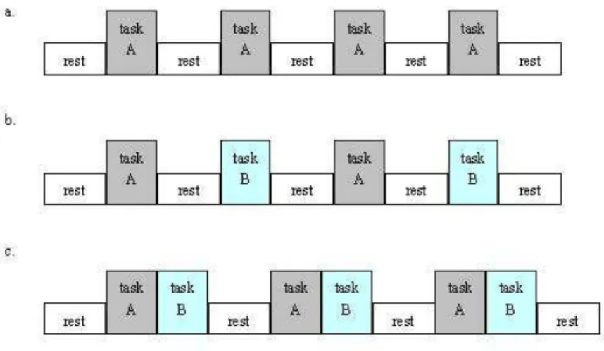
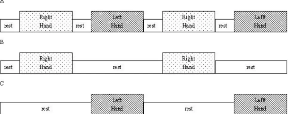
2.1 Examples of three different block designs . . . 5

2.2 A typical event-related design. A, B,... stand for different tasks . . . 6

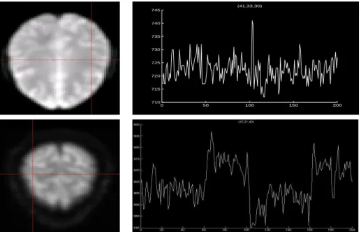
2.3 Examples of two time series corresponding to two different voxels recorded in an fMRI experiment. On each row, the left image shows a slice of the brain image with an example voxel indicated by the crossings of two lines. The right plot shows the time series related to the highlighted voxel. . . . 8

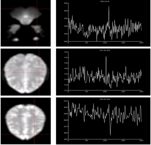
3.1 Examples of spikes in our fMRI data set. The left column contains the images for three slices of the brain. The right column plots the time series corresponding to the voxels highlighted by the line crossings on the slices. The big spikes around time points 110, 100 and 120 are examples of many other spikes in the data. . . 16

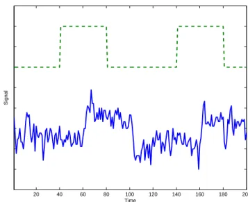
3.2 The recorded time course (solid line) of a voxel that is activated by the experiment stimulus sequence (dashed line). The lower and higher levels of the dashed line stand for rest and activation periods of the experiment respectively. . . 22

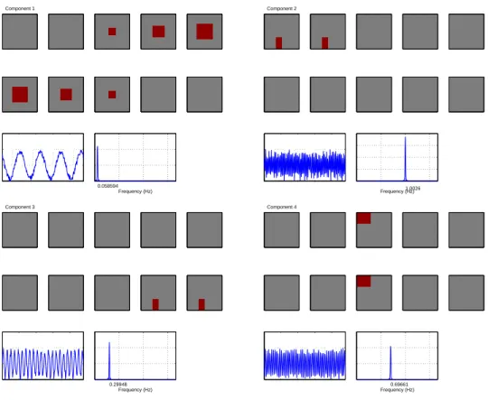
3.3 The first four components used in the simulation. In each panel, the first 10 images are the spatial component maps (one column of A), and the dark red areas stand for activated voxels. The solid line in the subsequent plot is the corresponding time series (one row of S). The dotted line stands for the rest-activation block design, 0 for “rest” and 1 for “active”. The spectrum plot for each time series is given at the end of each panel highlighting the frequencies. In this simulation study, Component 1 can be viewed as the one related to the experiment stimulus. Components 2 and 3 stand for heart beat and breath respectively. Component 4 could be an artifact effect. Component 5 is not shown here since it is pure noise. 28

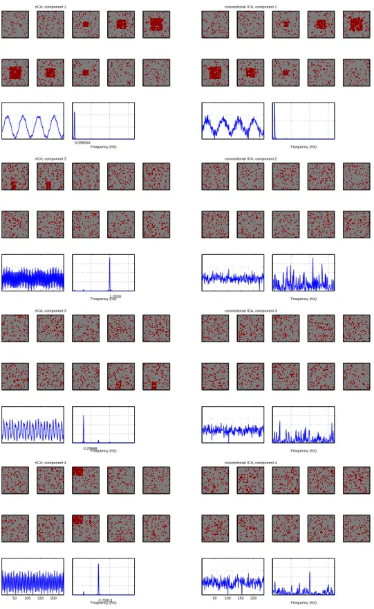
3.4 Comparison of the results from the proposed SSVD-ICA (the left column) and the conventional ICA (the right column). . . 30

(12)

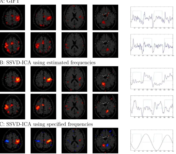
3.6 Activated brain regions and their corresponding temporal components de-tected by three methods, Panel (A): GIFT, right-hand (first row) and left-hand (second row); Panel (B): SSVD-ICA using estimated frequencies, right-hand (first row) and left-hand (second row); Panel (C): SSVD-ICA using specified frequencies, both right-hand and left-hand. Within each row, the first slice shows the primary motor cortex (PMC), the second slice contains both PMC andsupplementary motor area (SMA), the third slice shows basal ganglia and the fourth slice shows cerebellum. Red and blue areas illustrate the activated voxels. Brighter color indicates higher intensity. The last plot shows the corresponding time course with the hand-movement stimulus sequence overlayed. . . 32

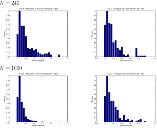
4.1 The histograms of the Amari distances obtained by applying Algorithm 2 using two ICA methods with sample size being 200, when the length of the simulated source signals is 240 and 1000 respectively. Top Left: KDICA with the length of the source signals 240; Top Right: SICA with the length of the source signals 240; Bottom Left: KDICA with the length of the source signals 1000; Bottom Right: SICA with the length of the source signals 1000. . . 41

5.1 The HRF modeled by Poisson distribution (left), Gamma distribution (middle) and Gaussian distribution (right). . . 46

5.2 The experiment stimulus sequence (left) is convolved with the canonical HRF (middle) to obtain one column of the design matrix X (right). . . . 48

5.3 The four components generated in the simulation. In each panel, the first 10 images are the spatial maps (one row of β), and the dark red areas stand for activated voxels. The solid line in the subsequent plot shows the temporal characteristic of the activated voxels (one column of X). The dotted line stands for the experiment stimulus, 0 meaning “rest” and 1 meaning “active”. . . 55

5.4 Comparison of the results from the proposed adaptive SPM approach (the left column) and standard SPM (the right column). . . 57

5.5 The experimental design used in acquiring the fMRI data. RE: EG Right-hand; RI: IG Right-Right-hand; LE: EG Left-Right-hand; LI: IG Left-hand. Each rest block took 30 seconds (10 scans when TR = 3 seconds). Each activation block took 60 seconds (20 scans). . . 58

(13)

5.6 Brain regions activated by the four finger movements detected by two methods, Panel (I): Adaptive SPM, EG hand (first row), IG right-hand (second row), EG left-right-hand (third row) and IG left-right-hand (fourth row); Panel (II): General SPM, EG right-hand (first row), IG right-hand (second row), EG left-hand (third row) and IG left-hand (fourth row). Within each row, the first slice shows the primary motor cortex (PMC), the second slice contains both PMC andsupplementary motor area(SMA), the third slice shows basal ganglia and the fourth slice shows cerebellum. Red areas illustrate the activated voxels. Brighter color indicates higher intensity. . . 60

5.7 The time components (solid lines) estimated by two methods with the stimulus sequence (dotted lines) overlayed. Left: Adaptive SPM; Right: General SPM with canonical HRF. . . 61

6.1 Left Panel: The recorded BOLD signal (solid line) triggered by a single event (dashed line). Right Panel: The recorded BOLD signal (solid line) triggered by a typical block-design sequence (dashed line). . . 63

6.2 The basic framework of the linear transform model. fMRI response is a linear transform of the neural activity. Adapted from Boyntonet al.(1996). 64

6.3 Linear addition of hemodynamic responses to individual stimulus events. Adapted from Dale and Buckner (1997). . . 65

6.4 An empirical shape of the hemodynamic response in fMRI to a single event stimulus. The four stages of the hemodynamic response are: A: lag-on; B: rise; C: decay; D: dip. . . 75

6.5 An example dataset from a simple event-related fMRI experiment. Within this time course: From time points 1−10, the subject was watching a dark display. At time points 11, a checkerboard pattern was presented 1500ms. After the offset of the checkerboard until time point 35, the subject was watching a dark display. . . 76

6.6 Top: the recorded BOLD signal; Middle: the estimated HRF by applying the new method; Bottom: dotted line – the recorded BOLD signal, solid line – the predicted BOLD signal by convolving the stimulus with the estimated HRF. . . 77

(14)

6.8 Top: dotted line – the recorded BOLD signal, solid line – the predicted BOLD signal by convolving the stimulus with the estimated HRF using our proposed method; Bottom: dotted line – the recorded BOLD signal, solid line – the predicted BOLD signal by convolving the stimulus with the estimated HRF using the basis function modeling in Fristonet al. (1995b). 79

6.9 The experiment paradigm. R: right-hand finger tapping; L: left-hand

fin-ger tapping. . . 79

6.10 The HRF modeled by SPM5 using a canonical HRF with time and dis-persion derivatives. . . 80

6.11 The four related slices that contain the areas activated by right-hand finger tapping. The first row consists of the t-maps generated by SPM5 and they don’t show any activation. The second row contains the p-maps generated by the proposed method. The first slice indicates the activated areas in cerebellum. The second slice contains basal ganglia. The third slice contains SMA and the fourth slice shows PMC. . . 80

6.12 The estimated HRFs for five voxels from PMC. . . 81

6.13 The estimated HRFs for three voxels from SMA. . . 81

6.14 The estimated HRFs for three voxels from cerebellum . . . 81

(15)

ABBREVIATIONS

AT _{transpose of} _A

BOLD Blood-Oxygenation-Level-Dependent

ER-fMRI Event-related fMRI

fMRI functional Magnetic Resonance Imaging

GLM General Linear Model

HRF Hemodynamic Response Function

ICA Independent Component Analysis

SPM Statistical Parametric Map

SSVD Supervised Singular Value Decomposition

(16)

CHAPTER 1

Introduction

Functional Magnetic Resonance Imaging (fMRI) is a set of noninvasive techniques for

functional brain mapping. By generating high quality “movies” of the brain in action,

it helps neuroscientists to study brain functions in vivo (Jezzard et al., 2001; Huettel

et al., 2004). Since early 1990s, it has gained growing popularity in both clinical and

basic neuroscience researches, and has influenced our understanding of the neurobiology

of human behavior.

The most popular fMRI technique makes use of blood-oxygenation-level-dependent

(BOLD) contrast, which is based on the differing magnetic properties of oxygenated

(diamagnetic) and deoxygenated (paramagnetic) blood. Simply speaking, increases in

local brain activity increase the local levels of blood oxygen. This in turn causes the

measured fMRI signal to increase. In a typical fMRI experiment, functional images are

recorded every few seconds while the subject is performing a specific task sequence or

receiving a series of stimuli. Because the images are taken using an magnetic resonance

(MR) sequence which is sensitive to changes in local blood oxygenation level, parts of the

images taken during a certain activation or stimulation would show different intensity.

And the parts of the images which show different intensity should correspond to the

parts of the brain which are activated by the certain stimulation. Through the BOLD

mechanism we can use fMRI data sets to answer two basic questions: (1) which brain

regions are responsible for certain cognitive functions of interest? (2) how do these brain

(17)

blood changes over time within an active brain region?

Since all measurements in the natural world are subject to random errors and an

image is a measurement, the images are subject to random errors too. This makes it

natural to involve fMRI studies with statistical analysis, which is concerned with making

inference about underlying features in data that contain a large amount of random errors.

Nowadays, statistics is playing a more and more active role in brain imaging science. To

help improve the overall quality of the design and analysis of fMRI experiments, statistical

techniques are required at almost all steps of fMRI analysis.

To date, a large variety of statistical procedures has been proposed for the analysis

of BOLD fMRI data. These methods include the most common univariate analysis and

multivariate methods. There are also parametric and nonparametric models considered.

From the point of view of time series analysis, there are time-domain and

spectral-domain methods. Although it has been demonstrated that some statistical procedures

outperform others in certain contexts, there does not exist a single, globally optimal

statistical method for the analysis of any particular fMRI study (Lange et al., 1999).

In this work, we focus on the study and improvement of three statistical techniques

that are most dominantly used in fMRI study. The first part of this work answers the first

question mentioned earlier, that is, which brain regions are activated by certain stimuli.

The key technique we use is independent component analysis (ICA) and we introduce

a supervised singular value decomposition (SSVD) method into the ICA procedure to

improve the robustness of ICA for fMRI data analysis against spikes which are common

in fMRI data.

In the second part, we study some popular ICA algorithms in the literature and

propose a bootstrap procedure to assess the variability of ICA estimates, which has not

been done in the literature. Using this proposed procedure, we can compare different

ICA algorithms as regard to reducing the variance of estimates.

(18)

statistical parametric mapping (SPM), to improve the estimation accuracy of the

tem-poral characteristic of the expected responses, and subsequently, the detection power of

activation.

The last part of this work handles the estimation of hemodynamic response by

mod-eling the hemodynamic response function (HRF). We propose a novel approach to detect

nonperiodic activations, estimate the HRF, and test the linearity assumption at the same

time.

The rest of this report is organized as follows. Chapter 2 is an overview of the fMRI

process, including the basic background of fMRI technique, the description of the fMRI

data structure and the role that statistics play in this particular field. More specifically,

detailed review of several most popular strategies developed for the analysis of BOLD

fMRI data is also provided.

In Chapter 3, we introduce our robust ICA procedure, which is developed to deal

with the spikes in fMRI data sets. Due to the high sensitivity of the MR scanner, spikes

are inevitable in acquiring the fMRI data, while they cause misleading effects for the

analysis. Currently in the literature, no particular methods are available for this issue.

Our method is proven to be powerful and advantageous for handling this spike-situation.

In Chapter 4, we present the bootstrap procedure for assessing the variability of

ICA estimates. We study two popular ICA algorithms and compare them through a

simulation study, using the proposed bootstrap procedure.

Chapter 5 describes the proposed adaptive SPM method to estimate the temporal

characteristic of the expected responses nonparametrically.

Chapter 6 introduces our novel approach for event-related fMRI study to model the

HRF nonparametrically and test the linearity assumption at the same time.

More thoughts about the future work in fMRI studies are discussed in Chapter 7 to

close this report.

(19)

CHAPTER 2

Overview of fMRI Analysis

2.1 Background

Back in 1890, the physiologist Arthur Sherrington originally demonstrated that local

neuronal activity is related to changes in brain metabolism and blood supply (Lange,

1996; Jezzard et al., 2001). This idea provides the basis for today’s

blood-oxygenation-level-dependent (BOLD) fMRI technique.

BOLD fMRI records signal contrast arising from the changes in magnetic

suscep-tibility of oxygenated and deoxygenated blood. The magnetic field applied in an fMRI

scanner is distorted to a different extent when it interacts with a different material. Since

oxygenated blood is diamagnetic and deoxygenated blood is paramagnetic, the measured

fMRI signal would increase when increases in local brain activity increase the local levels

of blood oxygen. This mechanism is how we can use the data collected from fMRI

ex-periments to localize specific areas of the brain that are activated by cognitive functions

of interest. For more detailed physics and physiology of BOLD fMRI, please refer to two

excellent introduction books Jezzard et al. (2001) and Huettelet al. (2004).

The fMRI techniques began to grow rapidly since the early 1990s, due to the increased

prevalence of MRI scanners and other related techniques. The range of applications of

(20)

brain mapping techniques.

2.2 General fMRI Process

An fMRI study usually starts with a question or hypothesis brought up by

neuroscien-tists. According to the question or hypothesis, proper fMRI experiments are designed and

implemented. Various related analyses are then carried out on the MR images recorded

during the experiments, to answer the question or test the hypothesis.

2.2.1 fMRI Experiment

There are some different strategies for fMRI experimental design available. The

ear-liest and most straightforward approach for comparing brain response to different tasks

during the imaging experiment is the “block design”. According to the practical goals

of the experiment, there could be one or more tasks involved and hence two or more

states included in the blocks. Each of these tasks or states lasts a certain continuous

time period and is performed in a certain order. Figure 2.1 shows several typical block

designs.

Figure 2.1: Examples of three different block designs

Another major method for fMRI experimental design, event-related design, has

be-come more and more popular recently. Different from traditional block designs, in

(21)

related designs, the stimuli are applied for short bursts in a stochastic manner. Figure

2.2.1 gives a typical example for event-related design.

Figure 2.2: A typical event-related design. A, B,... stand for different tasks

When evaluating the strengths and weaknesses of an fMRI experiment, two factors

are usually considered. The first is the detection power, that is, determining which brain

regions are activated by the experiment stimuli. Another factor is the estimation power,

which measures the pattern of blood changes over time within an active brain region

(Huettel et al., 2004). Both of the above experimental design strategies have their own

advantages and disadvantages as regard to these two factors.

In addition to its simple analysis, block design is very good for detecting significant

fMRI activity. But because the experimental conditions are extended in time, block

design is relatively insensitive to the shape of the hemodynamic response, and hence

poor at estimating the time course of blood changes in activated brain regions. On the

contrary, event-related design turns out to be very good at estimating the shape of the

hemodynamic response, while poor at the detection power.

Mixed designs that aim to combine both the block and event-related methods are

carried out too. They can best combine the detection and estimation power. But the

analysis of this kind of design is the most complicated too.

2.2.2 fMRI Data

During the fMRI experiment, a subject will lie in the magnet and perform a predefined

task sequence, while a certain number of MR images of the subject’s brain are typically

(22)

image consists of a certain number of slices and each slice is made up of individual cuboid

elements called voxels. Hence an fMRI data set can be considered as a three dimensional

matrix of voxels that is repeatedly sampled over time. Statistically speaking, an fMRI

data set is four dimensional and is usually represented as a spatio-temporal matrix X of

dimension M×N: each column ofX corresponds to an fMRI image withM voxels, and

each row ofX is a time series ofN time points for one voxel. This 4D fMRI data set can

then either be thought of as N volumes, one taken every few seconds, or as M voxels,

each with an associated time series of N time points. This is known as the complicated

spatio-temporal nature of the fMRI signals. In most fMRI experiments, the number of

time points is far less than the number of voxels (N ¿M).

Different analysis methods put emphasis on different aspects of fMRI signals. Some

methods think of the fMRI data in the spatial representation, while others think of them

in the temporal representation.

In Figure 2.3, we give two examples of the time series for two different voxels recorded

in an fMRI experiment. On each row, the left image shows a slice of the brain image

with an example voxel indicated by the crossings of two lines. The right plot shows the

time series related to the highlighted voxel.

2.2.3 Data Preprocessing

The 4D data set acquired by the MR scanner should go through a series of

prepro-cessing steps before it’s ready for any statistical analysis. These preproprepro-cessing steps take

the raw data as input, convert them into images that actually look like brains, then

reduce unwanted noise of various types, and precondition the data in order to aid the

later statistical analysis.

Usually the preprocessing consists of the following steps:

• Data reconstruction: The raw data are reconstructed into real space so that the image may be viewed and analyzed.

(23)

0 50 100 150 200 710

715 720 725 730 735 740 745

(41,33,30)

Figure 2.3: Examples of two time series corresponding to two different voxels recorded in an fMRI experiment. On each row, the left image shows a slice of the brain image with an example voxel indicated by the crossings of two lines. The right plot shows the time series related to the highlighted voxel.

• Slice-timing correction: Because each slice in each volume is acquired at slightly different times, it’s necessary to adjust the data so that it appears that all voxels

within one volume had been acquired at exactly the same time.

• Head motion correction: When the head moves during an experiment, some of the images will be obtained with the brain in the wrong location. The head motion

correction step is to adjust the time series of images so that the brain is in the

same position in every image. To accomplish this, each volume is transformed so

that the image of the brain within each volume is aligned with that in every other

volume. This step can be also called as a spatial normalization of the data.

• Intensity normalization: Each volume’s overall intensity level is adjusted so that all volumes have the same mean intensity. This intensity normalization can help

reduce the effect of global changes in intensity over time.

(24)

in the data.

• Temporal filtering: Each voxel’s time series is filtered by linear or non-linear tools in order to reduce the low and high frequency noise.

The basic goal of these preprocessing steps is to reduce unwanted variability in the

experimental data and to improve the validity of later statistical analyses (Huettelet al.,

2004). Without the preprocessing procedures, the statistical analysis would be greatly

reduced in power and even rendered invalid.

As important the data preprocessing is, it’s not the focus of our work. All the data are

preprocessed in the software package SPM5 (http://www.fil.ion.ucl.ac.uk/spm/) before

any statistical analysis in our work.

2.2.4 Statistical Analysis

After going through the sequence of preprocessing steps, the fMRI data is now ready

for the final statistical analysis. One main feature of fMRI data is that the signal changes

are small with the presence of lots of noise. This makes statistical analysis, which is

concerned with making inference about underlying patterns in data that often contain a

large amount of random error, necessary in fMRI analysis.

Over the last decade, a variety of statistical procedures has been proposed for the

analysis of BOLD fMRI data. One of the earliest and most direct ways is to simply

cross-correlate the voxel time series with a reference time course describing the sequence

of stimulant events in the experiment (Bandettini et al., 1993). The general linear model

(GLM) is another commonly employed procedure (Friston et al., 1994, 1995b). Lange

et al. (1999) compared nine analytic methods currently used in BOLD fMRI analysis.

Although it has been demonstrated that some statistical procedures outperform others in

certain contexts, there is no globally optimal statistical procedure for the analysis of any

particular fMRI study. More detailed review of the major statistical analysis methods is

given in the following section.

(25)

2.3 Common Statistical Analysis Techniques Review

Currently most popular statistical techniques for fMRI analysis can be differentiated

into two complementary categories, model-driven methods and data-driven methods.

These two kinds of strategies are based on different assumptions of fMRI data and have

their own advantages and disadvantages respectively.

2.3.1 Model-Driven Methods

The most widely used model-driven strategy for the analysis of fMRI data is statistical

parametric mapping (SPM), which is carried out using a two-stage approach. In the first

stage, a general linear model (GLM) with correlated errors is used for each voxel time

series. That is,

Yj =Xβj +²j, ²j ∼N(0, σ2Σ), j = 1,2, . . . , M, (2.1)

where M is the number of voxels of the brain. Yj is the time series of the jth voxel. The design matrix X contains terms that model the BOLD response to the stimuli and

non-linear trends that are often observed in fMRI voxel time series.

Once this model has been fitted at each voxel, inferences of the model parameters are

then made according to the experiment hypothesis. The resulting statistics from all the

voxels are assembled spatially into an image, which is the so-called statistical parametric

map. The second stage then focuses on the analysis of the statistical map in order to

identify those areas of the brain that are activated by the stimuli.

The generality of SPM comes mainly from the flexible forms of the design matrix

X and the variety of the statistics that can be calculated from the model. According

to the experimental design, the design matrix can contain both continuous covariates

and factorial indicators, which represent different effects of conditions in the experiment.

(26)

and blurred version of the stimulus design. Hence part of the design matrix X, which

represents the temporal characteristic of the expected responses, is commonly modeled

through the convolution of the stimulus designs(·) with ahemodynamic response function

(HRF), h(·). That is,

BOLD(t) = X u

h(t−u)s(u).

Commonly suggested forms for the HRF include discretized Poisson, Gamma and

Gaussian density functions. Most model-driven approaches for fMRI analysis can be

categorized as SPM, with different assumptions of the HRF, various forms of the general

linear model and different approaches for parameter estimation.

Fristonet al.(1994) gives a typical example of SPM analysis. This work identifies the

activated voxels by producing a statistical map with the voxel value being the correlation

coefficient between the observed fMRI signal and the input stimulus function. To consider

the effects of delay and dispersion of the hemodynamic response, the input stimulus is

first convolved with an HRF. The HRF is assumed to have a Poisson distribution, with

the mean being estimated using intrinsic autocorrelations in the observed fMRI signals.

Based on the estimation of the spectral densities of the observed fMRI signals and the

corrected (convolved with HRF) input stimulant signals in the spectral domain at each

voxel, this work calculates a statistic (ζ) which has a standard Gaussian distribution

under the null hypothesis (no effect in the voxel). Activated regions are then detected

by properly thresholding the resulted statistical parametric map with ζ values.

To allow for spatial variation in the HRF at each voxel, a small set of basis functions

can be used to model the HRF (Friston et al., 1995a; Josephs et al., 1997). Each basis

function is convolved with the design to make one column of the design matrix. Inferences

are then made on the linear model coefficients to form the statistical map.

In the paper by Lange and Zeger (1997), a non-linear parametric model for detecting

activations in fMRI data is presented. The model at each voxel is a special case of

Equation (2.1), with each column of the design matrix X being the convolution of a

(27)

stimulus sequence and an estimated HRF. The coefficient β_j shows the magnitude of the linear dependence of the observed fMRI signal at the jth voxel on the corrected

stimuli. Here the HRF is modeled as a two-parameter Gamma distribution whose Fourier

transform can be evaluated analytically. The two parameters of the HRF, which vary at

different voxels, are estimated simultaneously when estimating β_j. The analysis in this work is carried out in frequency domain too and the “non-linearity” resides in its iterative

way for estimating the parameters. Residual images are also obtained in this work. But

different from traditional SPM, where random field theory is used for global thresholding

to detect the activation regions, this work uses focused tests of activation. Namely,

the detection is focused on the potential activation areas given by neuroscientists. In

each of such region of interest (ROI), residual spatial autocorrelation functions (ACF)

are modeled by exponential and Gaussian forms. This modeling incorporates both the

spatial and temporal features of the fMRI data and gives the estimation of the

variance-covariance matrix W of the estimated βˆ. In each ROI, under the null hypothesis (no

any effect in that region) the statisticβˆ0_W−1_βˆ_{follows a}_χ2_{-distribution with degrees of}

freedom being the number of voxels in that ROI.

Bayesian analysis of fMRI data was first fully implemented in Genovese (2000).

In-stead of modeling the hemodynamic response by convolving the stimulus with a HRF

as in most studies, this work models the hemodynamic response directly in a Bayesian

framework. Four components are included in the voxelwise model, the baseline signal,

drift profile, activation profile and noise. Priors reflecting true prior knowledge are chosen

for the parameters involved in these four components. Spatial dependencies are included

in the noise model. One advantage of this method is that it produces estimates of

mean-ingful parameters instead of test statistics as in conventional SPM approaches, and hence

can answer questions beyond localization problem, e.g. monotonicity is considered as an

example in this work. MCMC algorithms are used for inferences, which also causes an

(28)

G¨osslet al.(2001b) also uses Bayesian analysis in fMRI and models the hemodynamic

response directly as in the above work. However this work adopts the regression model

used in Friston et al.(1994) instead and defines five different parameters for the signal’s

baseline, increase, plateau, decrease and undershoot. Prior distributions or numerical

values are then given to these parameters. Also based on a Bayesian framework, G¨ossl

et al.(2001a) proposed an approach for considering the temporal and spatial dependencies

between voxels, which is different from most SPM methods where the spatial correlations

between voxels are usually accounted for in the second step. Instead, the spatio-temporal

correlations are incorporated in the model formulation through spatial Markov random

field priors.

Marchini and Ripley (2000) proposed a nonparametric approach in spectral domain

for fMRI analysis. It is not a model-driven approach, but it can be viewed as a special case

in the SPM framework. This method is based on the fact that in periodic experimental

design, the fundamental frequency of activation contains the majority of information

regarding the observed response. Nonparametric techniques are used in all stages of the

analysis, including trend removal and correlation structure estimation. At each voxel, the

periodogram of the time series for the voxel and a smoothed version of this periodogram

are calculated to obtain the so-called ratio statistic. Inferences are then made based on

the ratio statistics for all the voxels. A small amount of spatial smoothing to the estimates

is applied to consider the spatial correlations. This nonparametric method takes least

assumptions about the original data compared with most parametric methods and is

more resistant to high frequency artefacts. The idea of this approach is illustrated by

periodic experiment examples, while it can be extended for event-related fMRI analysis

as well.

Some limitations of the above model-driven methods do exist. First of all, two

as-sumptions are required for GLM: normal distribution of the observed data and the

in-dependence of the error terms. Secondly, the validity of modeling the hemodynamic

(29)

response effect by the convolution model is yet to be verified. In addition, the forms of

the HRF commonly used in the literature are all predefined up to several parameters.

These subjective assumptions of the HRF may result in invalid estimates as well.

2.3.2 Data-Driven Methods

On the other hand, for exploratory fMRI analysis, data-driven approaches have been

found to be informative. These include clustering analysis (Goutteet al., 1999), principal

component analysis (PCA) (Kherif et al., 2002) and independent component analysis

(ICA) (McKeownet al., 1998b; Petersenet al., 2000; Calhounet al., 2003). Among these,

ICA is so far the most popular data-driven approach for block-design fMRI studies.

Different from model-driven methods, the data-driven methods are multivariate

tech-niques that account for the dependence among different voxels. In the following chapter,

we focus on the study of ICA, with more detail about the theory of ICA and its

advan-tages and disadvanadvan-tages.

More recently, SPM-ICA is proposed by Hu et al. (2005) to unify the model-driven

approach SPM with the data-driven approach ICA. In this work, temporal ICA (tICA)

was applied to fMRI data sets first to disclose independent components. The resulting

components are used to construct the design matrix of a GLM as in Equation (2.1). A

(30)

CHAPTER 3

Robust Independent Component Analysis

3.1 Introduction

ICA is a data-driven technique that aims to separate blind sources from their linear

mixtures based on the assumption of the statistical independence of the source signals.

McKeownet al.(1998b) originally introduced ICA to fMRI data analysis and this method

has attracted lots of interest in this field ever since. The literature body of the application

of ICA in fMRI studies has been growing rapidly.

As an exploratory data analysis tool, ICA is capable of extracting from the recorded

fMRI signals the individual signals that correspond to multiple sources such as

experiment-stimulus-related components, cardiac and respiratory effects and subject/machine

move-ments. However, most ICA algorithms are sensitive to outliers (McKeown et al., 1998b).

One of our contributions is to propose a technique that makes ICA more robust towards

outliers.

Outliers usually appear as spikes in fMRI data sets (Kao and MacFall, 2000). The

spikes refer to data points with relatively high signal magnitudes, and they are inevitable

in fMRI data sets due to radio-frequency problems in MR scanners, static discharge

caused by synthetic fibers or even abrupt subject movements. For illustration purposes,

Figure 3.1 plots the recorded time series corresponding to three different voxels in the

fMRI data set that we analyze later in Section 3.5. The big spikes around time points

(31)

0 50 100 150 200 280

285 290 295 300 305

(39,13,4)

0 50 100 150 200

710 715 720 725 730 735 740 745

(41,33,30)

0 50 100 150 200

850 860 870 880 890 900 910

(36,50,34)

Figure 3.1: Examples of spikes in our fMRI data set. The left column contains the images for three slices of the brain. The right column plots the time series corresponding to the voxels highlighted by the line crossings on the slices. The big spikes around time points 110, 100 and

120are examples of many other spikes in the data.

detected in fMRI data. The spatial locations of the voxels are respectively indicated by

the line crossings on the images in the left column. What is more interesting is that

the highlighted voxel in the first row even lies outside of the brain tissue; hence, the

corresponding spike clearly doesn’t represent any brain function. To the best of our

knowledge, there has not been much research explicitly addressing statistical issues with

the spikes. Luo and Nichols (2003) presented an exploratory diagnostic tool to identify

outliers in fMRI data sets.

(32)

A data reduction is usually performed through dimension reduction techniques such

as singular value decomposition (SVD) (Petersen et al., 2000). As mentioned earlier,

fMRI data sets are usually of high dimension and with far less time points than voxels.

Computationally, it is too expensive to apply ICA algorithms directly onto such matrices.

To make ICA more efficient, the data reduction aims at reducing the high-dimensional full

space to a much smaller feature subspace retained by SVD. Then the ICA decomposition

can be focused on the feature subspace. Section 3.2.2 gives more detail about this data

reduction step.

As a least squares based method, the SVD used for data reduction, however, is known

to be highly susceptible to outliers. Hence the analysis from the follow-up ICA could be

contaminated by those spikes. In this work, we propose a supervised SVD (SSVD)

pro-cedure that is less sensitive to the spikes in fMRI data sets. Our proposal is motivated

by the observation that SVD can be interpreted as a low rank matrix approximation

technique. The SVD components can then be obtained from solving a sequence of

min-imization problems. We introduce some regularization through basis expansion in the

corresponding optimization problems to achieve supervised low rank approximations.

The basis expansion is constructed using the information of the fMRI experiment

de-signs, particularly the frequencies of the stimulus sequences. Such supervision focuses

the SVD on the experimentally interesting directions, which makes the decomposition

more efficient and meanwhile less sensitive to spikes as illustrated in Sections 3.4 and 3.5.

The current research is motivated by one of the few fMRI studies focused on

elucidat-ing the neurocircuitry involved in Parkinson’s disease (PD) and its motor dysfunction.

PD patients can have trouble performing simple motor activities, such as finger tapping.

One research goal is to identify the brain regions (or Regions of Interest (ROIs)) that

are associated with finger tapping in these subjects. To detect all the ROIs associated

with performing motor activities robustly, this study employs a block design involving

alternating right/left-hand finger tapping (Figure 3.5). Our SSVD-ICA method makes

(33)

use of this design information.

The rest of this chapter is organized as follows. Section 3.2 provides an overview

of the ICA methodology as well as the conventional data reduction step before ICA. In

Section 3.3, we introduce the supervised SVD procedure and its application in ICA for

fMRI. Section 3.4 illustrates the performance of our proposed method using a simulation

study. In Section 3.5, we compare our method with an existing ICA package using one

fMRI data set collected in the aforementioned study. Concluding remarks are given in

Section 3.6 to close the chapter.

3.2 Independent Component Analysis

3.2.1 Overview of ICA for fMRI

ICA has been recently used in fMRI studies to extract independent source signals

from the recorded fMRI signals (McKeown et al., 1998b; Petersen et al., 2000; Calhoun

et al., 2003). The basic idea of ICA can be illustrated using the classic “cocktail party”

problem (Hyv¨arinenet al., 2001; Stone, 2004). Suppose many people talk simultaneously

at a party, and several microphones are recording in different locations. The recorded

signals are then mixtures of different voices. Using only these recorded mixtures as

inputs, ICA aims at identifying the individual voices of different people.

Mathematically, letxbe anM-dimensional vector variable, whose elements are signal

mixtures recorded at one time point, and s = (s1, . . . , sK)T be a K-dimensional vector variable with each element being a source signal at the time point. The typical ICA

model is written as

x=As, (3.1)

where A is an M ×K mixing matrix, M is the number of signal mixtures and K is the

number of source signals.

(34)

estimated only using the observed signal mixture x. For estimation purpose, the source

signalss1, . . . , sKare assumed to be statistically independent and have non-Gaussian dis-tributions. Hyv¨arinenet al. (2001) prove that, without the non-Gaussianity assumption,

the mixing matrix A is not identifiable at all.

According to the Central Limit Theorem, under certain assumptions, the

distribu-tion of the sum of several independent random variables is more Gaussian than any of

the original random variables. Making use of this fact, ICA recovers the independent

components by finding an unmixing matrixWto maximize the non-Gaussianity of Wx.

Then the mixing matrix A is estimated as W−1_{, and the source signals are recovered}

as s=Wx. For more detail about the theory of ICA, see Hyv¨arinen et al. (2001) and

Stone (2004).

As discussed earlier, an fMRI data set is usually represented as a spatio-temporal

matrix X of dimension M × N: each column of X contains an fMRI image with M

voxels recorded at one time point, and each row of X consists of a time series ofN time

points for one voxel. Adopting Equation (3.1) into the context of fMRI, we can write the

ICA decomposition model for X as:

X =AS, (3.2)

where each column of theM×K matrixA holds a spatial component map, each row of

the K×N matrixSis the corresponding time series, and K is the number of underlying

ICs or source signals.

Due to the spatio-temporal nature of fMRI signals, there are two distinct ICA

decom-position options, spatial ICA (sICA) and temporal ICA (tICA). The sICA aims to find

independent image components (the columns of A), while tICA looks for independent

time courses (the rows ofS). In either case, a single ICA component can be interpreted

as one spatially distributed set of voxels (one column of A) that is activated by the

(35)

corresponding time course in one row of S (McKeown et al., 2003).

3.2.2 The Data Reduction Step before ICA

fMRI data are usually of high dimension, especially in the spatial domain. In addition,

ICA algorithms are often computationally intensive. Hence before applying ICA, it is

common to first perform dimension reduction using SVD. ICA algorithms are then applied

in the reduced subspace.

Suppose rank(X) =r ≤min(M, N). The SVD decomposes X as follows,

X=UDVT, (3.3)

whereUis theM×r matrix oforthonormalleft singular vectors,V is theN×r matrix

of orthonormal right singular vectors, and D is the r ×r diagonal matrix of positive

singular values. Here Uand V can be viewed as the basis vectors that span the spatial

patterns and temporal sequences respectively.

As aforementioned, the sICA of X looks for independent image components, and

tICA for independent time series. Hence, when performing tICA, we can focus on the

subspace spanned by Y ≡ DVT_{, which is of dimension} _r_×_N_{, much smaller than the} originalM×N. Applying an ICA algorithm on the reduced dataY, we can getY = ˜AS,

where S contains the independent time components. The original spatial maps in the

model (3.2) can then be reconstructed as A=UA˜.

Similarly, sICA can be performed by focusing on the subspace retained byY∗ _≡_UD_.

An ICA decomposition on Y∗ _{results in} _Y∗ ₌_A_S˜_{, where} _A _{consists of the independent}

spatial maps. The original time courses in the model (3.2) are then recovered asS= ˜SVT_. In summary, the idea of the data reduction step before ICA is to reduce the dimension

of the matrices that will be used as inputs to ICA algorithms. Considering the fact

that most fMRI experiments have far less time points than voxels, i.e. r ≤ N ¿ M,

(36)

procedure.

3.3 Supervised Singular Value Decomposition

Both ICA and SVD are sensitive to spikes that are frequently encountered in fMRI

data. To overcome this analysis challenge, we propose to reduce the spike effect in the

data-reduction step via a modified SVD technique that is supervised by the experiment

design. Consequently, the follow-up ICA is more robust as it focuses on the subspace

maintained by the data reduction.

3.3.1 Low Rank Approximation via SVD

To motivate our approach, we note that SVD can be viewed as a matrix low rank

approximation method. In the SVD of X (3.3), let U = [u1, . . . ,ur], V = [v1, . . . ,vr] and D = diag{d1, . . . , dr}. For an integer l≤r, define

X(l)_≡

l

X

k=1

dkukvkT.

Then, X(l) _{is the closest rank-}_l _{matrix approximation to} _X _{(Harville, 1997). Let} _X∗

be an arbitrary rank-l matrix, the term “closest” simply means that X(l) _{minimizes the}

squared Frobenius norm betweenX and X∗_:

kX−X∗_k2

F = tr{(X−X∗)(X−X∗)T}.

Suppose, for example, we seek the best rank-one matrix approximation of X. Note

that any M ×N rank-one matrix can be written as uvT_{, where} _u _{is a norm-1}_M_-vector and v is a N-vector. The problem can be formulated as the following optimization

problem,

minu,vkX−uvTk2F. (3.4)

(37)

20 40 60 80 100 120 140 160 180 200

Signal

Time

Figure 3.2: The recorded time course (solid line) of a voxel that is activated by the experiment stimulus sequence (dashed line). The lower and higher levels of the dashed line stand for rest and activation periods of the experiment respectively.

Then SVD’s low rank approximation property implies the following solution

u=u1, v=d1v1.

The subsequent pairs (uk, dk,vk), k > 1, provide best rank-one approximations of the corresponding residual matrices. For example,d2u2v2T is the best rank-one approximation

of X−d1u1v1T.

3.3.2 Supervised SVD

In block design fMRI studies, experiment tasks or stimuli are typically applied in

alternating blocks. In the areas activated by these stimuli, we would observe temporal

data that are correlated with the experiment design. Figure 3.2 shows the time series

(solid line) of a voxel that is activated by the experiment stimulus (dashed line) in the

fMRI study reported later in Section 3.5. We note that the time components can usually

be modeled as sinusoidal curves plus some noise in such experiments. This observation

(38)

Suppose the time component of interest, v= (v(t1), . . . , v(tN))T, can be modeled as

v(ti) = asin(2πωti+φ) =acosφsin(2πωti) +asinφcos(2πωti),

where a is the amplitude, φ is the phase, ω is the frequency, and ti is the ith scanning time. Define

B= (b1,b2), ψ= (acosφ, asinφ)T,

where

b1 = (sin(2πωt1), . . . ,sin(2πωtN))T, b2 = (cos(2πωt1), . . . ,cos(2πωtN))T.

Then, one can see that

v=Bψ, (3.5)

which suggests that v is constrained to be in the linear space spanned by the bases b1

and b2.

To make use of the sinusoidal nature of v, we propose to impose the basis-expansion

constraint (3.5) onv in the optimization problem (3.4), and re-formulate the problem as

follows,

min

u,ψ kX−uv

T_k2

F subject tov=Bψ. (3.6)

We name this formulation Supervised SVD, because it supervises SVD by restricting it

to find the best low rank approximation within a certain subspace. On the other hand,

the conventional SVD is unsupervised.

One nice property of the formulation (3.6) is that it automatically achieves scale

invariant as indicated by

(cu)(v/c)T ={uc}{B(ψ/c)}T = (u)(Bψ)T =uvT,

(39)

where c is a nonzero constant. For identifiability purpose, we can standardize u and v

to unit length and introduce a slope parameter d. The problem can then be rewritten as

min

d,u,ψ kX−duv

T_k2

F subject tov=Bψ,uTu= 1,vTv= 1. (3.7)

Currently the SSVD is illustrated with only the base Fourier bases inB for simplicity

of the presentation. One can easily extendBto accommodate higher order Fourier bases,

which makes the methodology more flexible to model periodic signals.

3.3.3 Solution and Practical Implementation

The solution of the Supervised SVD (3.7) can be obtained by solving a couple of

generalized eigen-problems as stated below.

Theorem 1. The triplet {d,u,ψ} that minimizes (3.7) satisfies the following equations:

       

      

maxu uTXB(BTB)−1BTXTu subject to uTu= 1,

maxψ ψTBTXTXBψ subject to ψTBTBψ= 1,

d=ψTBT_XT_u_.

The proof of the theorem is relegated to Appendix A. The generalized eigen-problems

can be solved using standard methods as shown in the Appendix. Below we summarize

the computational algorithm to obtain the first supervised time component as well as

its corresponding spatial component. See the Appendix for the technical justification.

The same algorithm can be applied repeatedly on the residual matrices until the desired

(40)

Algorithm 1. Supervised SVD (SSVD)

(1) Obtain the frequency of interest ω from the experimenter, or estimate it through

spectrum analysis; (See the comments below.)

(2) Form the basis matrixBand apply Cholesky decomposition onBT_B_{to get}_BT_B₌

RT

BRB, where RB is a 2×2 upper triangular matrix;

(3) Apply SVD on XBR−1

B to derive its first left singular vector u and the first right

singular vector ˜ψ;

(4) Setψ≡R−1

B ψ˜ and d≡ψTBTXTu, which leads to v=Bψ. Hence we obtain the

first SSVD triplet {d,u,v}.

Below we want to comment on the choice of the sinusoidal frequency ω. The above

algorithm relies on knowing the sinusoidal frequency ω or being able to estimate it from

the fMRI data. In most fMRI experiments, the frequencyωof the interesting component

is known a priori, for example, the component corresponding to the experimental

stimu-lus. The experimenter might also be interested in some underlying unknown signals, in

which case we propose to estimate ω through spectrum analysis on the v components

extracted from the conventional SVD. The effect of spikes is trimmed by the fact that

they have a much smaller effect on the peak locations of the spectrums, or the dominating

frequencies of the signals.

3.3.4 Application to ICA

Once we obtain the desired number of SSVD components, we propose to apply an

ICA algorithm on them. As the SSVD components are insensitive to the spikes, the

analysis results from the follow-up ICA procedure should be robust as well (Section 3.4).

In addition, because our procedure (SSVD-ICA) makes use of the nature of the fMRI

experiment design, it appears to be more powerful in detecting activated brain regions

of interest (Section 3.5).

(41)

In terms of the number of SSVD components to extract, we propose the following

approach. If we know all the signal frequencies of interest, we can just extract the

corresponding components. Otherwise, we need to estimate the interesting frequencies.

For such, we suggest to extract the first 30 (for example) SVD components, and perform

spectrum analysis on them to identify possibly interesting frequencies, before applying

our SSVD approach. This approach is consistent with the common practice in ICA for

fMRI data, where around 20 or 40 ICA components are usually extracted, and interesting

components are then chosen either through visual inspection or correlation analysis.

3.4 A Simulation Study

To illustrate the robustness of the modified ICA using SSVD, we compare it with the

conventional ICA using SVD in the following simulation study.

3.4.1 Data Description

According to the ICA decomposition model (3.2), we simulated anM×N fMRI data

matrix X by first simulating the M ×K spatial component matrix A and the K ×N

time series matrix S separately. The data matrix X was then obtained as X=AS.

In this study, we set K = 5, M = 30×30×10 andN = 240. The simulated data can

be explained as follows: there are 5 underlying independent components; each column

of the spatial component matrix A is a component map that consists of 10 slices and

each slice contains 30×30 voxels; while each row of S is a time series of length 240 that

corresponds to the relevant spatial component in A. We simulated the data based on a

simple rest-activation block design (the dotted line in the time plot within each panel of

Figure 3.3). Each rest or activation period lasted 18 seconds.

Out of the five time components in the matrix S, the first four were simulated based

on simple sinusoidal functions plus randomly generated Uniform noise, which are plotted

in Figure 3.3 along with their corresponding spectrum plots highlighting the frequencies.

(42)

a frequency of 0.06Hz. The second and third time components are for the heart beat and

breath with frequencies of 1Hz and 0.3Hz respectively. The fourth one is an artifact effect

with a frequency of 0.7Hz. The last time component is pure noise. The amplitudes of

the first four components are 0.5, 0.45, 0.35 and 0.45 respectively. The noise is sampled

from a Uniform distribution between−0.1 and 0.1. Note that the noise distribution has

to be non-Gaussian in order for ICA to be well defined as discussed in Section 2.

All the voxels in A were given a numerical value of either 0 or 1. In each spatial

component, the voxels with value 1 correspond to the regions that were activated by the

corresponding time stimulus, and they are plotted as dark red areas in Figure 3.3.

To simulate spikes in the data, we randomly selected 10% of the entries in the

sim-ulated Xand replaced them with noise randomly generated from Uniform[−10,−2] and

Uniform[2,10]. The noise distributions are chosen so that the simulated spikes are indeed

outliers, judged by the usual 1.5-Inter-Quartile-Range rule of thumb.

3.4.2 Analysis and Results

Following the standard practice in ICA, we first normalized the contaminated data

matrix X by column centering and row standardization (Hastie and Tibshirani, 2002).

Both ICA and SSVD-ICA were applied to the normalized matrix. For computing, we

employed the fastICA algorithm (Hyv¨arinenet al., 2001) in both cases because of its fast

computation and popularity .

To effectively display the activated voxels in the extracted spatial maps, the values

in each map were standardized to z-scores (McKeown et al., 1998a) by subtracting the

component mean and then dividing the component standard deviation. Voxels with

|z| ≥1 were then identified as those activated by the corresponding stimulus, and they

were given value 1 while the voxels with |z|<1 were assigned as 0 when plotting.

The results from SSVD-ICA are shown in the first column of Figure 3.4. All the four

components can be recovered reasonably well, although some noise does exist. Similar

to Figure 3.3, dark red areas indicate the activated voxels. The time course plots in each

(43)

Component 1

Frequency (Hz) 0.058594

Component 2

Frequency (Hz)1.0026

Component 3

Component 4

(44)

panel show the corresponding time components, along with their spectrum plots.

The second column of Figure 3.4 shows the results from the conventional ICA.

Af-fected by the spikes, only the first component can be recovered; and the result is more

blurred than the corresponding one in the left column. The conventional ICA has trouble

identifying the remaining components.

3.5 A Real fMRI Data Analysis

3.5.1 Experiment Paradigm and Data Description

To study brain regions that are related to different finger tapping movements, an

fMRI data set was obtained from one human subject performing three different tasks

alternately: rest, right-hand movement and left-hand movement. Each rest period lasts

30 seconds and each activation period lasts 120 seconds. The experimental paradigm is

shown in Figure 3.5. Note the block design is used because the study is interested in

robustly identifying all the regions of interests involving the finger tapping.

During the experiment, two hundred MR scans were acquired on a modified 3T

Siemens MAGNETOM Vision system. Each acquisition consisted of 49 contiguous slices.

Each slice contained 64×64 voxels. Hence there were 64×64×49 voxels from each scan.

The size of each voxel is 3mm × 3mm × 3mm. Each acquisition took 2.9388 seconds,

with the scan to scan repetition time (TR) set to be 3 seconds.

3.5.2 Analysis and Results

The data set was preprocessed using SPM5. The preprocessing included realignment,

coregistration, segmentation, spatial normalization and smoothing. After the

preprocess-ing, we used the MATLAB functionshowsrsdeveloped by the Duke-UNC Brain Imaging

and Analysis Center (BIAC) to visually check the processed data set. Many spikes can

be easily seen, three of which are plotted in Figure 3.1.

We then applied both the proposed SSVD-ICA and ICA to the processed data set

after column centering and row standardization. When applying ICA, we employed an

(45)

rICA; component 1

conventional ICA; component 1

Frequency (Hz)

rICA; component 2

Frequency (Hz)

rICA; component 3

Frequency (Hz)

rICA; component 4

50 100 150 200

Frequency (Hz)

Temporal-spatial modeling for fMRI data