CONTRIBUTIONS TO PENALIZED ESTIMATION
Sunyoung Shin
A dissertation submitted to the faculty of the University of North Carolina at Chapel Hill in partial fulfillment of the requirements for the degree of Doctor of Philosophy in
the Department of Statistics and Operations Research in the College of Arts and Sciences.
Chapel Hill 2014
Approved by:
Jason P. Fine
Yufeng Liu
Michael R. Kosorok
J.S. Marron
ABSTRACT
SUNYOUNG SHIN: Contributions to Penalized Estimation (Under the direction of Jason P. Fine and Yufeng Liu)
Penalized estimation is a useful statistical technique to prevent overfitting problems.
In penalized methods, the common objective function is in the form of a loss function
for goodness of fit plus a penalty function for complexity control. In this dissertation,
we develop several new penalization approaches for various statistical models. These
methods aim for effective model selection and accurate parameter estimation.
The first part introduces the notion of partially overlapping models across
multi-ple regression models on the same dataset. Such underlying models have at least one
overlapping structure sharing the same parameter value. To recover the sparse and
overlapping structure, we develop adaptive composite M-estimation (ACME) by
dou-bly penalizing a composite loss function, as a weighted linear combination of the loss
functions. ACME automatically circumvents the model misspecification issues inherent
in other composite-loss-based estimators.
The second part proposes a new refit method and its applications in the regression
setting through model combination: ensemble variable selection (EVS) and ensemble
variable selection and estimation (EVE). The refit method estimates the regression
parameters restricted to the selected covariates by a penalization method. EVS
com-bines model selection decisions from multiple penalization methods and selects the
optimal model via the refit and a model selection criterion. EVE considers a
factor-izable likelihood-based model whose full likelihood is the multiplication of likelihood
The third part studies a sparse undirected Gaussian graphical model (GGM) to
explain conditional dependence patterns among variables. The edge set consists of
con-ditionally dependent variable pairs and corresponds to nonzero elements of the inverse
covariance matrix under the Gaussian assumption. We propose a consistent
valida-tion method for edge selecvalida-tion (CoVES) in the penalizavalida-tion framework. CoVES selects
candidate edge sets along the solution path and finds the optimal set via repeated
sub-sampling. CoVES requires simple computation and delivers excellent performance in
ACKNOWLEDGMENTS
First of all, I would like to express my deepest gratitude to my two advisors, Dr.
Jason Fine and Dr. Yufeng Liu. Without their guidance and support, this dissertation
would not be possible. Their keen insight and inspiring intuition have motivated me
to focus on this dissertation and pursue more research opportunities. The fruitful
academic discussions with them have made my research experience more enjoyable and
their invaluable advices have made my career path more clear.
Next I would like to thank my committee members, Dr. Michael Kosorok, Dr. J.
S. Marron, and Dr. Kai Zhang. I really appreciate that they have taken time out from
their busy schedule to serve as members of my committee. Their helpful advices and
comments have made this dissertation significantly better.
Last but not least, my sincere gratitude goes out to my friends and family. They
always believe in me and have encouraged me through my Ph.D. journey. With their
TABLE OF CONTENTS
LIST OF TABLES . . . ix
LIST OF FIGURES . . . xi
1 INTRODUCTION . . . 1
1.1 Background on Penalization . . . 1
1.1.1 Loss Functions in Penalized Estimation . . . 2
1.1.2 Properties and Computational Issues of Penalized Estimation . . . 7
1.2 New Contributions and Outline . . . 10
2 Adaptive Estimation for Partially Overlapping Models . . . 12
2.1 Introduction . . . 12
2.2 Oracle M-estimator for Overlapping Models . . . 16
2.2.1 Models and Notations . . . 17
2.2.2 Distinct Parametrization and Distinct Or-acle M-estimator . . . 19
2.2.3 Asymptotic Properties of Distinct Oracle M-estimator . . . 22
2.3 Adaptive Composite M-estimation for Overlap-ping Structure . . . 25
2.3.1 Choice of Penalty Functions . . . 25
2.3.2 Theoretical Results . . . 26
2.3.3 Choice of Weights and Tuning Parameters . . . 28
2.4.1 Classical Linear Regression Model . . . 31
2.4.2 Linear Location-Scale Model . . . 34
2.5 Baseball Data Analysis . . . 36
2.6 Discussion . . . 40
2.7 Proofs . . . 41
2.7.1 Proof of Lemma 2.1 . . . 41
2.7.2 Proof of Lemma 2.3 . . . 42
2.7.3 Proof of Theorem 2.1 . . . 42
2.7.4 Proof of Corollary 2.1 . . . 43
2.7.5 Proof of Lemma 2.4 . . . 43
2.7.6 Lemma 2.5 and Theorem 2.2 . . . 45
2.7.7 Proof of Theorem 2.3 . . . 49
3 Ensemble Variable Selection and Estimation . . . 51
3.1 Introduction . . . 51
3.1.1 Ensemble Variable Selection (EVS) . . . 52
3.1.2 Ensemble Variable Selection and Estima-tion (EVE) . . . 53
3.1.3 Outline . . . 54
3.2 Refitting for Variable Selection . . . 54
3.2.1 The Refit Method and Its Theoretical Properties . . . 55
3.2.2 Refit Least Squares Approximation (LSA) Estimation . . . 57
3.2.3 Simulation Studies . . . 60
3.3 Ensemble Variable Selection . . . 62
3.3.1 Ensemble of Decisions on Variable Selection . . . 63
3.3.3 South African Heart Disease Data Analysis . . . 70
3.4 Ensemble Variable Selection and Estimation . . . 72
3.4.1 Likelihood Factorization and Ensemble Estimation . . . 72
3.4.2 The Cox Proportional Hazards Model with Prospective Doubly Censored Data . . . 74
3.4.3 Simulation Studies . . . 77
3.4.4 Multicenter AIDS Cohort Study (MACS) Data Analysis . . . 82
3.5 Discussion . . . 89
4 Consistent Validation for Edge Selection in High Dimensional Gaussian Graphical Models . . . 90
4.1 Introduction . . . 90
4.2 Edge Selection in High Dimensional Gaussian Graphical Models (GGM) . . . 92
4.2.1 Settings and Notations . . . 92
4.2.2 Existing Methods . . . 93
4.2.3 Consistent Validation for Edge Selection (CoVES) Method . . . 95
4.3 Theoretical Properties . . . 99
4.3.1 Preliminary Steps . . . 99
4.3.2 Asymptotic Results . . . 100
4.4 Numerical Studies . . . 102
4.4.1 Double Chain Graphs . . . 103
4.4.2 Hub Graphs . . . 107
4.5 Discussion . . . 110
LIST OF TABLES
2.1 Simulation Results with Model Errors and
Num-bers of Correct Non-Zeros/Incorrect Zeros (n=100) . . . 32
2.2 Simulation Results with Model Errors and Num-bers of Correct Non-Zeros/Incorrect Zeros (n=500) . . . 33
2.3 Simulation Results with Grouping Ratios . . . 35
2.4 Regression Coefficients of Baseball Dataset . . . 39
2.5 Test Errors of Baseball Data for Three Quantiles . . . 40
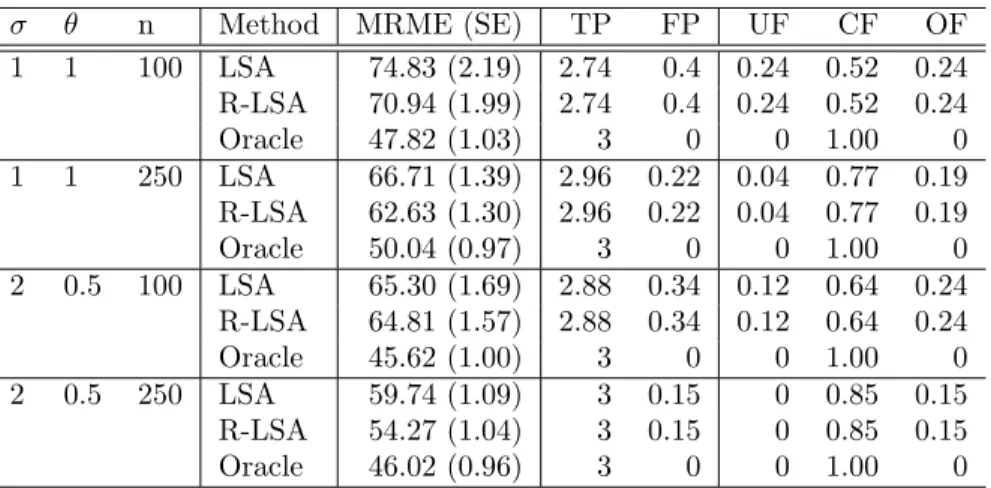
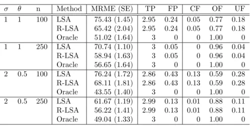
3.1 Refit LSA for Linear Regression Models . . . 61
3.2 Refit LSA for Median Regression Models . . . 62
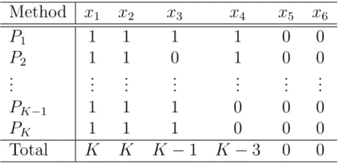
3.3 K Models Votes Table . . . 63
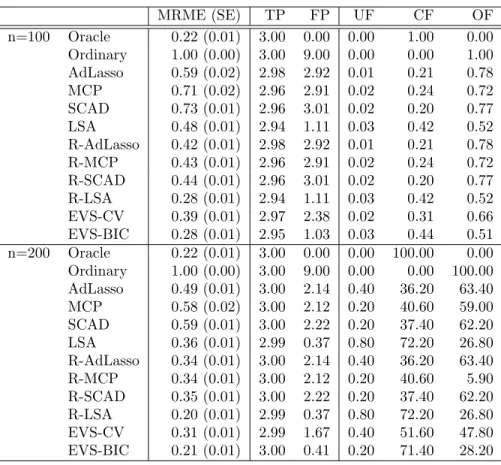
3.4 Simulation Results for Linear Regression (Gaus-sian Error) . . . 66
3.5 Simulation Results for Median Regression (Mix-ture Error) . . . 68
3.6 Simulation Results for Logistic Regression . . . 69
3.7 Optimal τ for Linear, Median, Logistic Regression . . . 70
3.8 Estimates and Standard Deviations for South African Heart Data . . . 71
3.9 Test Error for South African Heart Data . . . 72
3.10 Mean Squared Error of Estimators for Simulated Prospective Doubly Censored Data (n = 250) . . . 79
3.11 Mean Squared Error of Estimators for Simulated Prospective Doubly Censored Data (n = 500) . . . 80
3.12 Variable Selection Performance for Simulated Prospec-tive Doubly Censored Data . . . 81
3.14 Description of Risk Factors . . . 84
3.15 MACS Analysis with LTRC Data or CS Data . . . 86
3.16 MACS Data Analysis with Ensemble Methods . . . 88
4.1 Edge Selection Results for Double Chain Graph p= 10 . . . 104
4.2 Edge Selection Results for Double Chain Graph p= 40 . . . 105
4.3 Edge Selection Results for Double Chain Graph p= 50 . . . 106
4.4 Edge Selection Results for Double Chain Graph p= 100 . . . 106
4.5 Edge Selection Results for Hub Graph with p= 10 . . . 108
4.6 Edge Selection Results for Hub Graph with p= 40 . . . 108
4.7 Edge Selection Results for Hub Graph with p= 50 . . . 109
LIST OF FIGURES
1.1 Simple Undirected Graph Example (Lee 2013) . . . 7
1.2 Geometry of Lasso (p= 2) (Tibshirani 1996) . . . 8
2.1 Partially Overlapping Models . . . 13
2.2 Illustration of Distinct Parametrization withβ140 = β0 23 = 0 . . . 20
3.1 Prospective Doubly Censored Data . . . 75
3.2 Information Decomposition of Prospective Dou-bly Censored Data . . . 76
4.1 Double Chain Graph with p= 10 . . . 104
4.2 Double Chain Graph with p= 40 . . . 105
4.3 Double Chain Graph with p= 50 . . . 106
4.4 Double Chain Graph with p= 100 . . . 106
4.5 Hub Graph with p= 10 . . . 108
4.6 Hub Graph with p= 40 . . . 108
4.7 Hub Graph with p= 50 . . . 109
CHAPTER1: INTRODUCTION
1.1 Background on Penalization
In the past two decades, there have been significant developments in penalization
techniques, both in terms of methodology and applications. One of the most
popu-lar examples is the least absolute shrinkage and selection operator (Lasso) proposed
by Tibshirani (1996), which is closely related to nonnegative garrote (Breiman 1995).
Other examples include smoothly clipped absolute deviation (SCAD), elastic net and
adaptive Lasso. See Fan and Li (2001), Zou and Hastie (2005), Zou (2006) and Hastie,
Tibshirani, and Friedman (2001) and references therein for details.
We consider a training dataset with n independently and identically distributed random sampleszi = (xi, yi),i= 1,· · · , n, where xi ∈Rp is a vector of predictors and
yi ∈ R is the response variable. Our interest is to identify the underlying relationship
between the predictors and the response. Such a relationship is commonly learned
through a loss function, L(z,(α,βT)), where α ∈R is an intercept parameter,β ∈Rp
is a parameter vector of interest. In classical statistics, the estimator of the parameters
is the minimizer of the empirical loss function as below:
argmin
(α,βT)T
1
n
n
X
i=1
L(zi,(α,βT)). (1.1)
The loss function is used to measure the goodness of fit of the model on the data.
Some common examples of the loss term include the squared error loss in ordinary least
Penalized methods add a penalty term to (1.1), which controls the model complexity
to avoid overfitting. Many penalized methods can be cast as optimization problems.
The common objective function for optimization in a penalization method is in the
form ofloss+penalty as follows:
min
(α,βT)T
1
n
n
X
i=1
L(zi,(α,βT)) +λp(β), (1.2)
wherep(·) is the penalty function andλ≥0 is the regularization parameter. The regu-larization parameter determines the amount of penalty on the model complexity(Hastie,
Tibshirani, and Friedman 2001). A number of penalty functions have been developed
for sparse and structured estimation in numerous statistical models. For example, the
penalty function for Lasso is theL1-norm penalty, p
X
j=1
|βj|.
This chapter first discusses some loss functions and briefly examines penalization
methods. Section 1.1.1 reviews various loss functions and their corresponding statistical
models. Section 1.1.2 explores intuitions, properties, and computational algorithms of
penalization techniques.
1.1.1 Loss Functions in Penalized Estimation
Many loss functions are available for penalization methods. To address a statistical
problem, we may choose a suitable loss function. Several examples include least squares
loss, check loss, asymmetric least squares loss, composite loss and negative log-likelihood
loss for various statistical models. We first review them and briefly introduce related
penalization methods.
linear regression setup:
n
X
i=1
L(zi,(α,βT)) = n
X
i=1
(yi−α−xTi β)
2. (1.3)
Many studies on penalized methods started with this loss function and extended the
methods to other loss functions. Breiman (1995) and Tibshirani (1996) introduced
nonnegative Garrote and Lasso for the least squares loss function. These penalization
techniques have been adapted for likelihood-based regression, quantile regression, and
etc.
Koenker and Bassett (1978) introduced the quantile regression model to provide a
complete picture on the conditional distribution of the response. The τth conditional quantile function, fτ(x), is defined as P(y ≤ fτ(x)|x) = τ, for 0 < τ < 1 (Wu and
Liu 2009). We estimate theτth quantile as a linear function of the predictors with the check loss function:
n
X
i=1
L(zi,(α,βT)) = n
X
i=1
{τ(yi−α−xTi β)++ (1−τ)(yi−α−xTi β)−}, (1.4)
where t+ = tI(t ≥ 0) and t− = tI(t < 0). Some penalized methods for quantile regression were studied by Wu and Liu (2009) and Wang, Li, and Jiang (2007a).
Motivated by quantile regression, Newey and Powell (1987) proposed asymmetric
least squares regression. The check function is replaced with the asymmetric least
squares loss function:
n
X
i=1
L(zi,(α,βT)) = n
X
i=1
{τ(yi−α−xTi β) 2
++ (1−τ)(yi−α−xTi β) 2
−}. (1.5)
The τth expectile is defined as µτ(x) = ˆαaLS +xTβˆaLS, where ( ˆαaLS,βˆ T
minimizer of (1.5). It has the interpretation that the average distance from the
re-sponses, yi below µτ(x) to µτ(x) is 100τ% (Fan and Gijbels 1996). To our knowledge,
penalization methods for the asymmetric least squares have not been studied.
Recent studies on penalization have introduced a composite loss function, a weighted
linear combination of multiple loss functions. When we combine K loss functions, the composite loss function has the intercept parameters, αT = (α
1,· · · , αK) and
K parameter vectors of interest, β1,· · ·,βK. Most existing work assumes the same regression slope across the multiple losses, that is β =β1 =· · ·= βK ∈ Rp. Zou and
Yuan (2008) proposed the equally weighted composite quantile regression (EWCQR)
based on the following loss function:
n
X
i=1
L(zi,(α,βT)) = n
X
i=1
{
K
X
k=1
{τk(yi−αk−xTi β)++ (1−τk)(yi−αk−xTiβ)−}}, (1.6)
where 0 < τ1 < · · · < τK < 1. They developed the penalized EWCQR estimator
with the adaptively weighted L1 penalty. Bradic, Fan, and Wang (2011) introduced a
composite quasi-likelihood (CQ), a more general composite loss function. The CQ is a
weighted combination ofK convex loss functions,ρk(yi−α−xTi β),k = 1,· · · , K with
weightsw = (w1,· · · , wK). The corresponding loss function is written as follows:
n
X
i=1
L(zi,(α,βT)) = n
X
i=1
{
K
X
k=1
wkρk(yi−α−xTiβ)}. (1.7)
They proposed a robust and efficient penalized CQ estimator with theoretically optimal
weights.
Generalized linear model (GLM) is one of the well-known likelihood-based
ap-proaches. Suppose that yi has a density f(g(α+xTi β), yi) conditioning on xi, where
model as follows:
n
X
i=1
L(zi,(α,βT)) = − n
X
i=1
logf(g(α+xTi β), yi). (1.8)
GLM includes linear regression model, logistic regression model and poisson regression
model. Logistic regression is used for binary response modelling and poisson regression
is commonly used for count response modeling. For such models, Fan and Li (2001)
and Zou (2006) proposed SCAD and adaptive Lasso penalty functions.
Cox proportional hazards model is a popular semi-parametric model for survival
data (Cox 1972). The Cox model has a parameter of interest and a nuisance parameter,
(β,Λ). We first consider a simple model with right censoring. DenoteTi as the survival
time ofith observation andCias the subject’s right censoring time. Assume thatTiand
Ci are independent given xi. We observe n independently and identically distributed
samples of the triplet (Yi, δi,xi),i = 1,· · · , n, where Yi = min(Ti, Ci) and δi =I(Ti ≤
Ci). Furthermore, denote t1 < t2 < · · · < tN as N ordered observed event times and
(j) as the subject’s index corresponding to tj (Fan and Li 2002). The loss function for
the right censored data is the partial likelihood for the parameters of interest:
n
X
i=i
L(zi,(α,βT)) =− N
X
j=1
[xT(j)β−log{X
i∈Rj
exp(xTi β)}], (1.9)
where Ri is the risk set at time ti, Ri ={j :Yj ≥ti}. Tibshirani (1997) and Fan and
Li (2002) studied penalization methods for the partial likelihood-based Cox model.
Some survival models do not have an explicit partial likelihood form, such as Cox
frailty model and Cox models for interval or doubly censored data. We consider their
profile likelihood as an alternative, where the nuisance parameter is profiled out
profile likelihoods for the frailty model. Similarly, we can regularize the profile
likeli-hood with interval or doubly censored data. Note that these are challenging problems
since the corresponding profile likelihoods do not have closed form expressions (Fan
and Li 2002).
Undirected graphical models are known to be useful for explaining association
struc-ture in multivariate random variables (Lauritzen 1996, Drton and Perlman 2007). We
denote a graph as G = (V, E), where V ={x1,· · · , xp} is the set of vertices and E is
the set of edges between vertices. Each vertex corresponds to a variable and an edge
between vertices identifies their conditional dependence given all the other vertices.
Figure 1.1 shows a graphical model with five vertices, (x1, x2, x3, x4, x5) and four edges,
{(x1, x3), (x2, x3), (x3, x4) (x4, x5)}. The first edge, (x1, x3) implies that x1 and x3
are conditionally dependent given (x2, x4, x5). The other edges can be interpreted in
the same manner. Gaussian graphical models (GGM) impose a multivariate Gaussian
distribution to the p-dimensional vector, x= (x1,· · · , xp). Denote the distribution as
N(µ,Σ), where µ is a mean vector and Σ is a nonsingular covariance matrix. The corresponding loss function is the negative log-likelihood function:
−log|Θ|+ tr(SΘ), (1.10)
where Θ = Σ−1 is the precision matrix, S = 1
n
n
X
i=1
(xi −x¯)(xi −x¯)T is the sample
covariance matrix, and ¯x= 1
n
n
X
i=1
xi. The maximum likelihood estimator of Θ exists
and is unique with probability one ifn > p, and Buhl (1993) studied the case ofn < p. Estimating the structure of GGM is equivalent to recovering the support of the precision
matrix (Lauritzen 1996). Specifically, non-zero off-diagonal elements in the precision
the support of the precision matrix.
Figure 1.1: Simple Undirected Graph Example (Lee 2013)
1.1.2 Properties and Computational Issues of Penalized Estimation
Penalized estimation can perform simultaneous variable selection and estimation
with a proper choice of the penalty function. Tibshirani (1996) gave an intuitive
expla-nation on the sparse estimation for the Lasso. Assume that each predictor is
standard-ized to have mean zero and variance one. The Lasso intercept estimate is
n
X
i=1
yi/n and
the Lasso estimate for β, ˆβ, is determined by the following constrained optimization
problem
min
β
1
n
n
X
i=1
(yi−xTi β)2 subject to p
X
j=1
|βj| ≤t, (1.11)
where t is the tuning parameter. Note that the loss term in (1.11) can be rewritten as 1
n(β−
ˆ
βls)TXTX(β−βˆls) plus a constant, where ˆβls is the ordinary least squares estimate and X = [x1,· · · ,xn]T. Figure 1.2 illustrates its elliptical contours and the
constraint as the black square for p = 2. The Lasso estimate is the coordinate that the contours first touch the square. It will be sometimes on the axes, and hence a zero
coefficient can be obtained via the Lasso.
Many penalization methods have the general formulation of penalized estimation in
Figure 1.2: Geometry of Lasso (p= 2) (Tibshirani 1996)
problem:
min
β
1
n
n
X
i=1
(yi−xTi β) 2+λ
d
X
j=1
|βj|. (1.12)
It is the summation of a least squares loss function and L1 norm penalty. Another
example is the graphical Lasso (glasso) for sparse inverse covariance estimation
(Fried-man et al. 2008). It is known to be useful for explaining association structure in
high-dimensional data such as gene expression data and microRNA data. We
regular-ize the negative log-likelihood for GGM in (1.10) with the L1-penalty over a positive
definite constraint:
min
Θ>0−log|Θ|+ tr(SΘ) +λ||Θ||1, (1.13)
where ||Θ||1 is the L1-norm, the sum of the absolute values of the elements of Θ. We
estimate the true edge set of the GGM with a proper choice of tuning parameter, and
then obtain a sparse GGM.
The penalty functions in penalized estimation can be roughly categorized into two
classes: convex penalty functions and nonconvex penalty functions. The convex
penal-ties such as Lasso and adaptive Lasso have computational advantage since the
cor-responding optimization problems have convex objective functions. The nonconvex
penalties might have theoretical advantage over the convex penalties, but their
SCAD penalty, the minimax concave penalty (MCP), and the folded concave penalties
are common examples of the nonconvex penalties. Further details on these penalty
functions can be found in Fan and Li (2001), Zhang (2010) and Fan, Xue, Zou, et al.
(2014).
The theoretical properties of penalized estimation have been studied in the
liter-ature. Certain penalization methods such as SCAD and adaptive Lasso satisfy the
desirable theoretical properties (Fan and Li 2001, Zou 2006). These are known as the
oracle properties since the methods asymptotically perform as well as the oracle
esti-mator, which knows the true model in advance (Donoho and Johnstone 1994). The
oracle procedures have consistency in variable selection and asymptotic normality of
the nonzero coefficients with the same efficiency as the oracle estimator.
Computational algorithms have been intensively studied for many penalization
methods. Efron, Hastie, Johnstone, and Tibshirani (2004) proposed a powerful least
angle regression (LARS) algorithm, an advanced version of forward selection with the
least squares loss. The computational cost for the entire solution path is of the same
order as the full ordinary least squares. Its simple modification calculates Lasso and
adaptive Lasso estimates with the least squares loss. Zou and Li (2008) developed a
unified algorithm based on local linear approximation (LLA) for the nonconvex
penal-ties with negative log-likelihood loss. The proposed one-step LLA estimator from the
algorithm reduces the computational burden. Friedman, Hastie, and Tibshirani (2010)
suggested a coordinate-wise descent algorithm for the convex penalized least squares
regression and GLM. Later, Breheny and Huang (2011) studied its applications to the
nonconvex penalties for the least squares regression and the logistic regression. Given
the tuning parameter, each step of the algorithm is applied to a single parameter with
the remaining parameters fixed, and the updated solution is used as a warm start for the
in GGM (Friedman, Hastie, and Tibshirani 2008).
1.2 New Contributions and Outline
The contribution of this dissertation is to give new insights on penalized
estima-tion in various statistical models. We propose some new methods with theoretical
investigation and extensive numerical studies. The outline of the proposal is as follows:
• Chapter 2 introduces the notion of overlapping structure in a composite loss function and defines partially overlapping models for several models of
inter-est. We develop the oracle M-estimator for partially overlapping models and
establish its theoretical properties. Furthermore, we suggest adaptive composite
M-estimation, regularized estimation for the sparsity and overlapping structure
recovery of the overlapping models. The method is theoretically justified and
numerically demonstrated as competitive against several existing methods with
composite loss functions.
• Chapter 3 first introduces the refit method, a simple two-step procedure based on a penalization method. Based on the refitting, we propose ensemble
vari-able selection (EVS) and ensemble varivari-able selection and estimation (EVE). EVS
obtains candidate refit estimators according to voting results from several
penal-ization methods and chooses the optimal one by a certain information criterion
or cross-validation. Numerical studies illustrate that EVS can often identify the
best penalized method in each scenario. Next, EVE is studied for a factorizable
likelihood-based model in the penalization framework. In such a model, the full
likelihood can be factorized into distinct likelihood factors. EVE is a multi-step
procedure based on information combination across the factors, the refitting, and
(2007). We perform numerical studies for simulated prospective doubly censored
data and analyze Multicenter AIDS Cohort Study (MACS) data with EVE.
• Chapter 4 studies the edge selection for sparse high-dimensional undirected GGM. We develop consistent validation for edge selection (CoVES) motivated by
con-sistent cross-validation for generalized linear models in Feng and Yu (2013). Its
underlying target is a sparse graph model, where a small number of variables
are conditionally dependent. CoVES first obtains the candidate edge structures
from the entire glasso solution path. For each selected graph structure, CoVES
computes the empirical negative log-likelihood via repeated random subsampling
validation. Finally, CoVES selects the edge structure having the smallest negative
log-likelihood as the optimal structure. We study its asymptotic property under
growing sample size with fixed dimension and show its competitive performance
CHAPTER2: ADAPTIVE ESTIMATION FOR PARTIALLY OVERLAPPING MODELS
2.1 Introduction
Regression modeling has been a popular statistical tool to explain the association
between a response variable and covariates in a dataset. A statistical regression model
targets a profile of the conditional distribution of the response given the predictors.
We estimate conditional mean of response as a linear function of predictors in classical
linear regression while we estimate conditional median as a linear function of predictors
in median regression. It is of great interest to consider several linear models to describe
a more complete picture of the conditional distribution. We may simultaneously fit
the models on the dataset and estimate the parameters. Such joint estimation borrows
information across the models and is referred as to composite estimation.
The composite estimation may be based on combing loss functions as weighted
averages of loss functions tailored to individual models. Givennindependent identically distributed samples, z1 = (x1, y1),· · · ,zn= (xn, yn)∈Rp ×R, consider the following
K different empirical convex loss functions to each model:
1
n
n
X
i=1
Lk(zi,(αk,βk))≡
1
n
n
X
i=1
Lk(yi, αk+xiTβk), k = 1,· · · , K, (2.1)
whereαk’s are the different intercept terms across the models andβ1,· · · ,βK ∈Rp are
for the loss functions. Our composite loss function is formulated as:
L(zi,(αT,βT))≡ K
X
k=1
wkLk(yi, αk+xTi βk), (2.2)
where α = (α1,· · ·, αK)T, β = (βT1,· · · ,β T
K)T ∈ RK×p, and w = (w1,· · · , wK)T is
a positive weight vector. Note that minimizing (2.2) without further assumptions on
parameter overlap is equivalent to minimizing the loss functions separately. The loss
functions may have the same or different forms. For example, in composite quantile
regression (CQR), each Lk is a check function with the arguments toLk being used to
fit models to different quantiles (Zou and Yuan 2008). For the τ-th quantile, Lτ(t) =
τ t++ (1−τ)t−, where t+ =tI(t ≥0) and t− =tI(t <0) respectively. Combining the check function for median regression with the usual least squares loss function yields
an example of composite loss functions derived from different Lk.
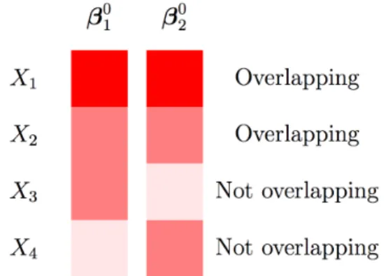
Figure 2.1: Partially Overlapping Models
Composite estimation is useful when the underlying parameter structures are
par-tially overlapped. In the parpar-tially overlapping models, some parameters are the same
across loss functions, while others are different. Overlap may occur between two or
more loss functions. Figure 2.1 shows a simple example of the partially overlapping
models. Each parameter vector corresponds to both loss functions (β1 and β2). The
same parameter values (β1 and β2) to both loss functions. We call this arrangement
overlapping structure. According to the definition of overlapping structure, the third
and fourth covariates in this example do not overlap across the models. The fourth
element of β1 and the third element of β2 demonstrate sparse structure. They appear
white-shaded, which indicates that they are zero-valued parameters. Both CQR and
L1-L2 loss functions may have overlapping parameter vectors for different quantiles or
median and expectation, depending on the effects of the covariates on the variance
function.
A complete overlapping structure is one extreme of partially overlapping structures,
where all parameters are common to all loss functions. For the completely overlapping
models, Bradic, Fan, and Wang (2011) and Zou and Yuan (2008) used the composite loss
functions, with the goal of improving efficiency of the regression parameter estimators.
Their composite loss function has the following form:
L(zi,(αT,βT))≡ K
X
k=1
wkLk(yi, αk+xTi β), (2.3)
where α ∈ RK and β ∈
Rp. The composite loss in (2.3) is identical to that in (2.2),
except that the regression slopes are the same for different k. Such M-estimation has been studied for efficient and sparse estimation when the underlying model follows a
classical linear model. The assumption leads to completely overlapping models, where
the individual loss functions have a common parameter vector. Note that the
exist-ing methods do not consider each loss as a model, but rather consider the composite
loss function as an approximation of the unknown log-likelihood function of the error
distribution (Bradic, Fan, and Wang 2011).
The completely overlapping modeling in composite loss estimation (Bradic et al.
model whose several covariates affect the scale of response and its error is centered to
zero but not symmetric. Different loss functions estimate different parameters defined
both by the mean and variance of the response. The parameters are the same for the
covariates which have no effect on the variance function (Carroll and Ruppert 1988).
Parameter vector for L2 is the same as the regression parameter vector of the model
while parameter vector for L1 is the weighted sum of the regression parameter vector
and the scale parameter vector. Other examples in which different loss functions may
correspond to models with partially overlapping parameters include composite quantile
regression (CQR), in which multipleL1 loss functions are linked to different quantiles.
In this chapter, we aim for the efficient composite estimation under weaker
as-sumptions on the overlapping structure, the partially overlapping structure. To adapt
such overlapping structure in the models, we incorporate penalization into (2.2). The
penalty is applied to all absolute pairwise differences between coefficients corresponding
to each covariate. In addition to this grouping penalty, we also employ a penalty for
sparse estimation, as in Bradic et al. (2011). The objective function for our empirical
composite loss function with double penalties is
K
X
k=1 n
X
i=1
wkLk(yi, αk+xTi βk) +n K
X
k=1 p
X
j=1
pλ1n(|βkj|) +n
X
k<k0
p
X
j=1
pλ2n(|βk0j−βkj|). (2.4)
The penalty terms in (2.4) applied to the difference in the coefficients enable recovery of
the overlapping structure by shrinking small differences towards zero. The penalty term
applied to each coefficient encourages sparsity by shrinking small coefficients towards
zero. One should recognize that the penalization of the differences is used not for
variable selection, but for selecting the overlapping structure across the multiple loss
functions. The fused lasso (Tibshirani, Saunders, Rosset, Zhu, and Knight 2004) also
pairwise penalty serves a different purpose, that of identifying local consistency of
coefficients in a single model.
In the sequel, we propose and study adaptive composite M-estimation (ACME)
based on (2.4) which simultaneously shrinks towards the true overlapping model
struc-ture while estimating the shared coefficients in that strucstruc-ture. As in Bradic et al. (2011),
our procedure yields estimators with improved efficiency by information combination
across the models. Our procedure correctly selects both the true overlap structure
and the true non-zero parameters in the true model structure with probability 1 in
large samples. The parameter estimators hereby obtained are oracle in the sense that
they have the same distribution as the oracle estimator based on knowing the true
model structure a prior, both the true overlapping parameters and the true non-zero
parameters.
The rest of the chapter is organized as follows. In Section 2.2, we introduce notation
for the distinct parameter vector across models, based on overlap in the βk’s, and
define the oracle estimator. The large sample properties of the oracle estimator are
established under partially overlapping models. Section 2.3 presents ACME for partially
overlapping models and describes its implementation along with a rigorous discussion
of its theoretical properties. Section 2.4 contains numerical results from an extensive
simulation study and Section 2.5 reanalyzes a well known dataset on the annual salaries
of professional baseball players. All proofs are relegated to Section 2.7.
2.2 Oracle M-estimator for Overlapping Models
Before discussing our procedure, it would be helpful to understand the underlying
model and the oracle estimator. Oracle procedures estimate the parameters of
inter-est when the underlying parameter structure is known in advance (Fan and Li 2002).
estimation with constraints on the sparsity and overlapping structure. We first
intro-duce notations and settings for partially overlapping models and investigate theoretical
properties of the oracle estimation.
2.2.1 Models and Notations
We first consider the K separate models with their corresponding loss functions in (2.1). The risk function for the kth model is defined as the expectation of kth loss function, Rk(αk,βk) = Ez[Lk(y, αk +xTβk)] for βk ∈ Rp, k = 1,· · · , K. The true
parameter vector for thekth model is the minimizer of the corresponding risk function,
Rk(αk,βk), with (α0k,β 0T
k )T = argmin (αk,βTk)T∈Θ⊂Rp+1
Rk(αk,βk). We estimate the parameter
vector of each model by minimizing its corresponding loss function. Consider a stack
of all parameter vectors across all models, and define the K·(p+ 1)-dimensional true parameter vector as (α0T,β0T)T = (α0
1,· · · , α0K,β 0T
1 ,· · · ,β 0T K )T.
Next we describe the underlying parameter structure across the multiple models
with set notations. We can identify the underlying sparse and overlapping structure
with sparsity sets and overlap sets. Denote Ak = {j ∈ {1, . . . , p} : βkj0 6= 0} as the
index set of the non-zero parameters to the kth model and Ac
k = {1, . . . , p}\Ak as
its complement. This set notation implies β0Ac
k = 0 ∈ R |Ac
k|, k = 1,· · · , K, and thus
describes the sparse structure of the modelk. Note that the underlying sparse structure for all models can be obtained from the collection of the nonzero parameter index sets,
A0 ≡ {A k}Kk=1.
We further introduce notations between two models for the overlapping structure
illustration. Denote Okk0 = {j ∈ {1, . . . , p} : β0
kj = βk00j 6= 0} as the index set of the
same valued non-zero parameters betweenβ0kand β0k0 fork6=k0. Note that elements of Okk0 corresponds to non-zero same valued parameters to the modelk and the modelk0.
for all model pairs, O12,· · · ,O1K,O23,· · · ,OK−1,K. In other words, the underlying
overlapping structure can be illustrated from the collection of the overlapping index
sets, G0 ≡ {O
kk0}k6=k0. Consider a collection of all possible overlappings, Γ = {G}G∈Γ.
The true grouping, G0, is an element of Γ.
With the true sparse structure,A0, we can decompose the parameters into two parts
for partially overlapping models. The first part is for the entire true zero parameters,
βAc
k = [βkj]j∈A c k ∈ R
|Ac
k|, and the second part is the entire true non-zero and intercept
parameters, (αT,βTA)T = (αT,βTA1,βTA2, · · · , βTAK)T, where βAk = [βkj]j∈Ak. Note
that the true parameter vector for all models, (αT,βT)T, corresponds to the union of the two parts, (αT,βT
A)T and βAc
k,k = 1,· · · , K.
For joint estimation, we define the composite loss function as the linear combination
of all loss functions with weights in (2.2). The composite risk function is the expectation
of the composite loss function asR(αT,βT) = E
K
X
k=1
wkLk(αk,βk) = K
X
k=1
wkRk(αk,βk).
Note that the composite risk function is a weighted linear combination of all risk
func-tions and is separable into K risk functions. Hence, the minimizer of the composite risk function,R(αT,βT), is the true parameter vector for all K models: (α0T,β0T)T =
argmin
(αT,βT)T∈Θ⊂
RK·(p+1)
R(αT,βT
). The composite risk function can be viewed as the risk function of the parameter vector across all models. Note that the true non-zero and
intercept parameter vector is the minimizer of the composite risk function restricted to
the non-zero parameters with the overlapping constraint:
(α0T,β0TA )T = argmin
(αT,βT A)T
K
X
k=1
wkRk(αk,βAk) (2.5)
subject to βAkj =βAk0j ∀j ∈ Okk0, ∀k < k 0
,
whereRk(αk,βAk) = EzLk(y, αk+x
kTβ
Ak) andx
k
The oracle M-estimator of (αT,βT)T for partially overlapping models is the unpe-nalized M-estimator obtained under the assumption that the sparsity and overlapping
structure is known in advance. Denote the oracle estimator as ( ˆαoT,βˆoT)T. Similar to
the true parameters, we have the decomposition of the oracle estimator into the zero
parameter part and the non-zero parameter part:
ˆ
βoAc k = [β
o kj]j∈Ac
k =0|Ack|∈R |Ac
k|
( ˆαoT,βˆoTA )T = ( ˆαoT,βˆoTA1,· · · ,βˆoTA K)
T ∈ RK+
PK
k=1|Ak|, where ˆβo Ak = [β
o kj]j∈Ak.
The first part estimates the true zero parameters of all models and the second part
estimates the true non-zero and intercept parameters. Since we know the sparsity
pattern of the models,Ac
1,· · · ,AcK, we estimate the corresponding parameters as zeros.
Analogous to the definition of the true parameters in (2.5), the oracle estimator to the
non-zero parameters minimizes the empirical weighted multiple loss functions with the
overlapping structure constraint:
( ˆαoT,βˆoTA )T = argmin
(αT,βT A)T
1
n
n
X
i=1 K
X
k=1
wkLk(yi, αk+xkTi βAk)
subject toβAkj =βAk0j ∀j ∈ Okk0, for anyk < k 0
.
2.2.2 Distinct Parametrization and Distinct Oracle M-estimator
The common parametrization in Section 2.2.1 includes the duplication of the same
valued parameters from overlapping structures. That is, the parametrization is
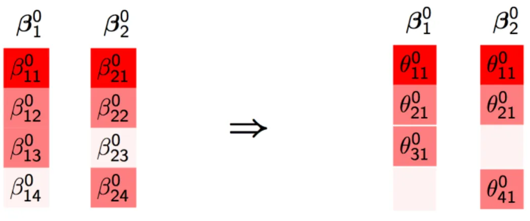
redun-dant for partially overlapping models. The left panel of Figure 2.2 shows an
exam-ple of such redundant parametrization. We use two 4-dimensional parameter vectors,
β1,β2 ∈R4, to describe the models from Figure 2.1. The first parameter pair,β 11 and
same value. We can use one parameter,θ11, forβ11andβ21, and another parameter,θ21,
for β12 and β22 as in the right panel of Figure 2.2. Furthermore, this parametrization
excludes the zero-valued parameters, β23 and β14. We call such parametrization
dis-tinct parametrization or non-redundant parametrization. The underlying sparse and
overlapping structure is imposed on the non-redundant parametrization for the true
non-zero and intercept parameters. The distinct parametrization is used for a lower
dimensional formulation of the oracle M-estimator.
Figure 2.2: Illustration of Distinct Parametrization withβ0
14 =β230 = 0
To define our distinct oracle estimator, we borrow the notations from Bondell and
Reich (2007) for the parametrization. Consider the union of the index sets of the
non-zero parameters of all models,
K
[
k=1
Ak ={j1,· · ·, jQ}. It corresponds to the index set of
covariates with a non-zero true parameter in at least one model. Denote its cardinality
as Q = |
K
[
k=1
Ak|, which is less than or equal to the number of covariates, p. Given a
variable, xjq, jq ∈
K
[
k=1
Ak, consider the unique true non-zero parameter values among
the elements of {β0
Akjq :∀k s.t. jq ∈ Ak}. They are called the true distinct parameters
to the variable, xjq. For example, we have
K
[
k=1
Ak ={1,2,3,4}for the models in Figure
2.2. The first two covariates, x1 and x2, have one true non-zero parameter value from
{β0
11, β210 } and {β120 , β220 } respectively since we have β110 = β210 and β120 = β220 . For the
and β240 , respectively.
Suppose we have theGq(≤K) true distinct parameters denoted asθq10 ,· · · , θqG0 q for q= 1,· · · , Q. We denote the true distinct parameter vector across all covariates as
θ0 = (θ00,θ10,· · · ,θ0Q)T
= (θ010 , · · · , θ00K, θ011, · · · , θ01G1 · · ·, θQ10 , · · · , θ0QG Q)
T ∈ RK+
PQ
q=1Gq,
where θ00 = (θ010 , · · · , θ00K)T is the true intercept vector, α0. The true distinct pa-rameter vector is the non-redundant enumeration of the true papa-rameters in terms of
overlapping structure for all models along the predictors.
We can define the distinct composite loss function with the non-redundant
parametriza-tion as L(zi,θ) = K
X
k=1
wkLk(yi,θ0k+xkTi βAk(θ)), where [βAk(θ)]j is an element of θ
corresponding to βAkj, j ∈ Ak. The distinct composite loss function is a random
con-vex function on RK+PQq=1Gq. The distinct composite risk function is the expectation of
the distinct composite loss function withR(θ) =Ez[L(z,θ)] =
K
X
k=1
wkRk(θ0k,βAk(θ)).
Note that the minimizer of the distinct composite risk function is the true distinct
parameter vector.
The distinct oracle M-estimator of θ is defined as the minimizer of the distinct loss
function as follows:
ˆ
θo = (ˆθ01o , · · · , θˆ0Ko ,θˆo11, · · · , θˆo1G1, · · · , θˆoQ1, · · · , θˆQGo Q)
T
= argmin
θ
1
n
n
X
i=1
L(zi,θ)∈RK+ PQ
q=1Gq.
We assume that the dimension of the distinct oracle M-estimator, K +
Q
X
q=1
Gq, is less
Specifically, every element of ˆθoq (q = 1,· · · , Q) corresponds to some nonzero elements among ˆβ1joq,· · · ,βˆKjo q when they are overlapped. Conversely, every nonzero element among ˆβo
1jq,· · ·,
ˆ
βo
Kjq corresponds to one element of ˆθ
o q.
2.2.3 Asymptotic Properties of Distinct Oracle M-estimator
Before introducing ACME in Section 2.3, we establish the asymptotic properties
of the distinct oracle M-estimator in Section 2.2.3. For the theoretical properties, the
following assumptions on allK separate loss functions are required.
A1. (α0 k,β
0T
k )T = argmin (αk,βTk)T∈Θ⊂Rp+1
ELk(y, αk+xTβk), k = 1,· · · , K are bounded and
unique.
A2. ELk(y, αk+xTβk)<∞ for each (αk,βTk)∈Rp+1, k= 1,· · · , K.
A3. a) Lk(y, αk +xTβk) is differentiable w.r.t. (αk,βTk)T at (αk0,β 0
k) for Pz-almost
every z = (x, y) with derivative ∇(α
k,βTk)TLk(y, αk+x
Tβ0 k) and
Jk(αk0,β 0
k)≡E[∇(αk,βTk)TLk(y, αk+x
T
β0k)· ∇(αk,βT
k)TLk(y, αk+x
T
β0k)T]<∞.
b) The risk functionRk(αk,βk) = E[Lk(y, αk+xTβk)] is twice differentiable w.r.t.
(αk,βTk)T at (α0k,β 0T
k )T with a positive definite Hessian matrix, Hk(α0k,β 0 k).
A4. The loss function, Lk(y, αk+xTβk), is convex with respect to (αk,βTk)T for Pz
-almost every z.
Similar conditions can be found for one model setting in Section 2.1 of Rocha, Wang,
and Yu (2009). The assumption, A1, ensures that the parameter for the kth model, (α0
k,β 0T
k )T, is well defined. The second assumption, A2, guarantees that the pointwise
limit of the loss function is the risk function. FromA3, we can consider local quadratic
approximate the loss function to the risk function at each point near the parameter.
The last assumption, A4, is used to apply Convexity Lemma (Pollard 1991) for the
uniformity of approximation.
Lemma 2.1 shows that the composite loss function of (2.3) satisfies the same
as-sumptions asA1-A4 if all loss functions,L1,· · · , LK, satisfy the assumptions. In other
words, the composite loss function automatically satisfies the desirable properties for
such approximation.
Lemma 2.1. If all loss functions, Lk(y, αk+xTβk), k= 1,· · · , K, satisfy the
assump-tions, A1,· · ·,A4, then the composite loss function, L(zi,(αT,βT)) also satisfies the
same assumptions.
Next we present Lemma 2.2 under the same assumptions for theoretical investigation
of the oracle M-estimator and ACME. We prove consistency and asymptotic
normal-ity of the distinct oracle M-estimator and √n-consistency, selection and overlapping consistency, and asymptotic normality of ACME in Section 2.3.2.
Lemma 2.2. If each loss function, Lk(y, αk +xTβk), k = 1,· · · , K, satisfies the
assumptions, A1-A4, then
(a) There exists a K ·(p+ 1) dimensional random vector W ∼ N(0, J(α0T,β0T
))
such that
n
X
i=1
[L(zi,(α0T,β0T)+
uT
√
n)−L(zi,(α
0T,β0T))]−[1
2u
T·H(α0T,β0T)·u+WT·u]→p 0
for each u∈RK·(p+1)
(b) For every compact set K ⊂RK·(p+1),
sup
u∈K
||
n
X
i=1
[L(zi,(α0T,β0T) +
uT
√
n)−L(zi,(α
−[1 2u
T ·H((α0T,β0T
))·u+WT ·u]||→p 0
Lemma 2.2 shows the pointwise convergence and the uniform convergence of the
loss,
n
X
i=1
[L(zi,(α0T,β0T) +
uT √
n)−L(zi,(α
0T
,β0T))]. It is a generalization of Lemma 2 of Rocha et al. (2009), which considers the setting of a single loss function.
The distinct oracle M-estimator is a special type of M-estimators based on the
distinct loss function. Its asymptotic properties are established using M-estimation
theories.
Lemma 2.3. If the loss assumptions, A1-A4, are satisfied for all K separate loss
functions, then θˆo converges in probability to θ0 as n→ ∞.
Lemma 2.3 shows the consistency of the distinct oracle M-estimator, which is used
for Theorem 2.1. It states that the distinct oracle M-estimator has the asymptotic
normality.
Theorem 2.1. If the loss assumptions, A1-A4, are satisfied for all K separate loss functions, then
√
n(ˆθo−θ0)→d N(0,H(θ0)−1J(θ0)H(θ0)−1)), as n→ ∞ where [H(θ0)]ij =
∂2R(θ)
∂θi∂θj
|θ=θ0, and J(θ0) = E[∇θL(z,θ0)∇θL(z,θ0)T].
The non-redundant oracle estimator across models asymptotically follows a normal
distribution, similar to some oracle estimators based on a single model. We can extend
the results for the original estimators as shown in Corollary 2.1.
Corollary 2.1. If the above assumptions are satisfied, then √n( ˆβoA k −β
0
Ak) = Op(1)
From Corollary 2.1, we also have√n−consistency of the composite oracle estimator, ˆ
βoA. The asymptotic property is preserved because the oracle estimator for each model
is a subset of the distinct oracle estimator.
2.3 Adaptive Composite M-estimation for Overlapping Structure
The joint estimation procedure, ACME, improves the performance of all models as
it shares the information across the multiple models. The penalized estimation recovers
the true parameter structure in terms of the sparsity and overlapping. The two penalty
terms in ACME objective function, (2.4), control the sparsity and overlapping level.
2.3.1 Choice of Penalty Functions
For the two penalty terms,pλ1n(|t|) andpλ2n(|t|), we consider folded concave penalty
functions and weightedL1 penalty functions. First, the general folded concave penalty
functions on t∈[0,∞) satisfy the conditions below (Fan, Xue, Zou, et al. 2014)
(i) pλ(t) is increasing and concave in t∈[0,∞);
(ii) pλ(t) is differentiable in t∈(0,∞) withp0λ(0) :=p
0
λ(0+)≥a1λ;
(iii) p0λ(t)≥a1λ for t∈(0, a2λ];
(iv) p0λ(t) = 0 for t∈[aλ,∞) with the pre-specified constant a > a2,
wherea1 anda2are some fixed positive constants. The penalty function is differentiable
Forθ >0, the first derivative of the SCAD penalty is
p0λ(θ) =λI(θ ≤λ) + (aλ−θ)+
(a−1)λ I(θ > λ),
wherea >2 andλ >0 are tuning parameters (Fan and Li 2001). We commonly select
a = 3.7. Note that SCAD has a1 = 1 and a2 = 1 in the form of the folded concave
penalty functions. MCP is defined as
pλ(θ) = λ
Z θ
0
(1− x aλ)
+dx,
with a tuning parameter a > 1. MCP hasa1 = 1−a−1 and a2 = 1 in the form of the
folded concave penalty functions (Zhang 2010).
The weighted L1 penalties take the form of p0λ(|θˆ(0)|)|θ|, where ˆθ(0) is a consistent
estimator of θ0. The weighted L
1 penalty function provides a one-step local linear
approximation estimator (Zou and Li 2008). We consider two types of the preliminary
penalty functions for the weightedL1 penalty functions, pλ(t). The first function is the
folded concave penalty and the second one is pλ(t) = λp(t), where p0(t) is continuous
on (0,∞) and there is some s > 0 such that p0(t) = O(t−s) as t → 0+. Additionally, the adaptive Lasso penalty is obtained by lettingp0λ(ˆθ(0))≡λ|θˆ(0)|−s, wheres >0 (Zou
2006). We adopt the one-step SCAD penalty in numerical studies for both steps in
Section 2.4.
2.3.2 Theoretical Results
We establish the theoretical properties of ACME under the assumptions, A1-A4,
on all models. We develop the asymptotic theories based on the objective function in
(2.4), which is denoted as Qn(αT,βT). In particular, we focus on the oracle properties
Lemma 2.4. If λ1n →0, λ2n →0 for folded concave, one-step folded concave penalty
functions, and √nλ1n → ∞,
√
nλ2n→ ∞ for weighted L1 penalty functions, there is a
local minimizer of Qn(αT,βT) such that
√
n|( ˆαT,βˆT)T −(α0T,β0T)T|=Op(1).
If both pλ1n(t) and pλ2n(t) are weighted L1 penalty functions, then ( ˆα
T,βˆT)T is the
unique global minimizer.
Lemma 2.4 demonstrates the existence of a √n-consistent penalized M-estimator with a proper choice of λn. We control the magnitude of Qn((αT,βT) +uT/
√ n)− Qn(αT,βT) for a sufficiently large |u| to show the selection and overlapping
consis-tency in Theorem 2.2. The notion of overlapping consisconsis-tency is analogous with that
of selection consistency. We achieve the overlapping consistency and both ˆβkj and ˆβk0j
have the exactly same values for any index j ∈ Okk0 with probability tending to 1.
Theorem 2.2. Suppose that λ1n →0, λ2n→ 0,
√
nλ1n → ∞,
√
nλ2n→ ∞ for folded
concave, one-step folded concave penalty functions. For weighted L1 penalty functions,
suppose √nλ1n→0,
√
nλ2n→0, n
s+1
2 λ1n → ∞, n
s+1
2 λ2n→ ∞. If there exists at least
one j ∈ Okk0 for some k < k0, then P(
K
\
k=1
\
j∈Ac k
{βˆkj = 0} ∩
\
k<k0
\
j∈Okk0
{βˆkj = ˆβk0j}) →1
as n → ∞.
Theorem 2.2 implies that the ACME achieves selection consistency and overlapping
consistency. Let ˆAk = {j ∈ {1,· · · , p} : ˆβkj 6= 0} denote as the non-zero coefficient
index set corresponding to the kth loss function. Denote ˆG as the estimated group-ing. The selection and overlapping consistency can be written as P({Aˆk = Ak, k =
1,· · · , K} ∩ {Gˆ=G0})→1.
Let ˆθA0(G0) denote our distinct ACME from (2.4) provided we know the true
distribution of ˆθA0(G0) since our estimator selects the true K models and has the true
overlapping structure with probability tending to one. Note that its dimension is same
as the dimension of the distinct oracle estimator.
Theorem 2.3. If the assumptions in Theorem 2.2 are satisfied, then
√
n(ˆθA(G0)−θ0)
d
→N(0,H(θ0)−1J(θ0)H(θ0)−1)).
Theorem 2.3 states that the distinct estimator has the same asymptotic distribution
as the distinct oracle estimator in Theorem 2.1. The ACME across the multiple models
follows a normal distribution in terms of non-zero non-redundant enumeration as the
penalized estimators of a single model for the non-zero parameters follow a normal
distribution (Fan and Li 2001).
2.3.3 Choice of Weights and Tuning Parameters
The asymptotic distribution of the distinct ACME in Theorem 2.3 leads to
theoreti-cal optimal weights to achieve the efficiency across the multiple models. The theoretitheoreti-cal
criterion for the choice of weights is to maximize the efficiency of the estimator (Bradic
et al. 2011). We can use the determinant of the asymptotic covariance matrix of the
estimator or its trace as the criterion. Note that its asymptotic covariance is a function
of the unknown matrices ofJ(θ0) and H(θ0), and both depend on the weight vector,
w. Similarly, completely overlapping models also have the asymptotic normal
distribu-tion and their asymptotic covariance depends on the weight vector (Bradic et al. 2011).
In this underlying classical linear model setup, the asymptotic covariance matrix can
be simplified as the multiplication of a scalar function and a function of predictors.
The scalar function has the weight vector and the random errors of the model as its
matrix. Bradic et al. (2011) chooses the weight vector by minimizing the function.
However, such decoupling cannot be obtained for partially overlapping models, due to
the complex form of the asymptotic covariance.
To address the problem, we suggest a data dependent approach to select weights.
We first obtain the separate penalized M-estimators as the initial separate estimators
with
ˆ
β(0)k = argmin
(αk,βTk)T∈Θ⊂Rp+1
n
X
i=1
Lk(yi, αk+xTi βk) +n p
X
j=1
pλ1n(|βkj|), k= 1,· · ·, K.
The preliminary M-estimator achieves sparse estimation, but does not attain
overlap-ping estimation. Note that zero-estimated parameters can be estimated as non-zero
in the ACME procedure. Next we calculate data-driven weights, w = (w1,· · · , wK)T
based on the preliminary estimators. We setwk to be proportional to the reciprocal of
the empirical loss function of the initial estimators with
wk ∝[
1
n
n
X
i=1
Lk(yi, αk+xTi βˆ (0) k )]
−1, k= 1,· · ·, K.
We recommend this weight ratio for the same leverage of each loss function to the
composite loss function. For computational efficiency, they are rescaled to have sum to
one as
K
X
k=1
wk = 1. We adopt this choice of weights in numerical studies of Section 2.4,
which yields excellent performance. We assume positive weights because the presence of
a zero weight automatically removes the parameter vector of the corresponding model.
To obtain the optimal tuning parameters for λ1n and λ2n, we use 5-fold
cross-validation (Fan and Li 2001). Denote the full dataset by T = {z1,· · · ,zn}. We
randomly divide T into the five test sets, T1, · · · , T5. Then, their corresponding
training sets areT −T1, · · ·, T −T5. We obtain the ACME from thevth training set
T −Tv as ( ˆα(v)T,βˆ (v)T
parameter pairs by minimizing the following cross-validation criterion:
CV(λ1n, λ2n) = 5
X
v=1
X
zi∈Tv
K
X
k=1
Lk(yi,αˆ (v)
k +x
T i βˆ
(v) k )
Lk(yi,αˆ (0)
k +xTi βˆ (0) k )
.
A two dimensional grid search is performed for the selection of (λ1n, λ2n).
2.4 Simulation Studies
We first perform simulation studies under a classical linear model and a linear
location-scale model. Each dataset in Sections 2.4.1-2.4.2 is generated from both of
these two models. We obtain ACME for both least absolute deviations (LAD) regression
and least squares (LS) regression with a composite L1-L2 loss function. We compare
it with separate LAD and LS estimators such as ordinary unpenalized LAD and LS
estimators (Ordinary), adaptive Lasso penalized LAD and LS estimators (AdLasso),
and one-step SCAD penalized LAD and LS estimators (SCAD). We also compare with
penalized composite quasi-likelihood (PCQ) in Bradic et al. (2011), which is developed
for a classical linear model. PCQ assumes the completely overlapping structure across
all loss functions.
For comparison, we report the median of model errors (MME), the standard error of
model errors (SE), the number of correctly classified non-zero estimators (TP), and the
number of incorrectly classified zero estimators (FP). The model error of each estimator
is defined as M E( ˆβ) = ( ˆβ−β0)T
E(XTX)( ˆβ−β0). We also evaluate the overlapping
performance across the LAD and LS models. The overlapping structures are categorized
into four types: truly grouped estimators, truly grouped non-zero estimators, truly
grouped zero estimators, and truly ungrouped estimators. Denote the index set of each
category as TG, NG, ZG, and UG respectively. Since TG is partitioned into NG and
|NG|/|TG| and |ZG|/|TG|.
2.4.1 Classical Linear Regression Model
In this section, we consider the classical linear model from Fan and Li (2001):
yi =xTi β 0+
i,
where β0 = (3,1.5,0,0,2,0,0,0,0,0,0,0). The covariate xi is multivariate normal
with zero mean and covariance, Cov(xij1, xij2) = 0.5|j1−j2|, 1 ≤ j1, j2 ≤ 12. Suppose
that the error term, 1,· · · , n, follows a normal distribution (N(0,3)), a double
expo-nential distribution (DE), and a t distribution with d.f. 4 (t(4)). We consider both LAD regression and LS regression. In this case, the true models are completely
over-lapped since the true parameter vector of the LS regression is the same as the true
parameter vector of the LAD regression. For these models, both PCQ and ACME
use the composite L1-L2 loss function. Our choice of weight for ACME is (w1, w2) ∝
(1/M AE( ˆαSCADlad ,βˆSCADlad ),1/M SE( ˆαSCADls ,βˆSCADls )),whereM AE( ˆαSCADlad ,βˆSCADlad ) is the mean of absolute errors of the SCAD-LAD estimator andM SE( ˆαSCAD
ls ,βˆ SCAD
ls )) is the
mean of squared errors of the SCAD-LS estimator. The results are obtained from 100
simulated datasets with n = 100 and n = 500. We use 5-fold cross-validation for the tuning parameter selection.
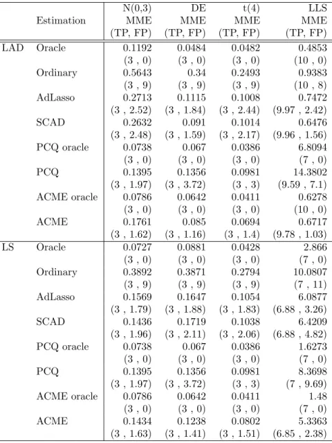
From the first three columns of Tables 2.1 and 2.2, the performance of ACME is
the best for both L1 and L2 under DE error with n = 100,500 and under t(4) with
n = 100 in terms of MME. Under N(0,3) with n = 100,500, the MMEs of the PCQ are smaller than those of ACME, but ACME outperforms the others. In this setting,
PCQ is generally comparable to ACME because PCQ achieves the oracle overlapping
structure. All the estimators successfully select the significant variables, β0
evidenced by TP. ACME performs the best in terms of FP in most cases.
N(0,3) DE t(4) LLS
Estimation MME MME MME MME
(TP, FP) (TP, FP) (TP, FP) (TP, FP)
LAD Oracle 0.1192 0.0484 0.0482 0.4853
(3 , 0) (3 , 0) (3 , 0) (10 , 0)
Ordinary 0.5643 0.34 0.2493 0.9383
(3 , 9) (3 , 9) (3 , 9) (10 , 8)
AdLasso 0.2713 0.1115 0.1008 0.7472
(3 , 2.52) (3 , 1.84) (3 , 2.44) (9.97 , 2.42)
SCAD 0.2632 0.091 0.1014 0.6476
(3 , 2.48) (3 , 1.59) (3 , 2.17) (9.96 , 1.56)
PCQ oracle 0.0738 0.067 0.0386 6.8094
(3 , 0) (3 , 0) (3 , 0) (7 , 0)
PCQ 0.1395 0.1356 0.0981 14.3802
(3 , 1.97) (3 , 3.72) (3 , 3) (9.59 , 7.1)
ACME oracle 0.0786 0.0642 0.0411 0.6278
(3 , 0) (3 , 0) (3 , 0) (10 , 0)
ACME 0.1761 0.085 0.0694 0.6717
(3 , 1.62) (3 , 1.16) (3 , 1.4) (9.78 , 1.03)
LS Oracle 0.0727 0.0881 0.0428 2.866
(3 , 0) (3 , 0) (3 , 0) (7 , 0)
Ordinary 0.3892 0.3871 0.2794 10.0807
(3 , 9) (3 , 9) (3 , 9) (7 , 11)
AdLasso 0.1569 0.1647 0.1054 6.0877
(3 , 1.79) (3 , 1.88) (3 , 1.83) (6.88 , 3.26)
SCAD 0.1436 0.1719 0.1038 6.4209
(3 , 1.96) (3 , 2.11) (3 , 2.06) (6.88 , 4.82)
PCQ oracle 0.0738 0.067 0.0386 1.6273
(3 , 0) (3 , 0) (3 , 0) (7 , 0)
PCQ 0.1395 0.1356 0.0981 8.3698
(3 , 1.97) (3 , 3.72) (3 , 3) (7 , 9.69)
ACME oracle 0.0786 0.0642 0.0411 1.48
(3 , 0) (3 , 0) (3 , 0) (7 , 0)
ACME 0.1434 0.1238 0.0802 5.3363
(3 , 1.63) (3 , 1.41) (3 , 1.51) (6.85 , 2.38)
Table 2.1: Simulation Results with Model Errors and Numbers of Correct Non-Zeros/Incorrect Zeros (n=100)
In this setting, we have TG={1,2,· · · ,11,12}, NG={1,2,5}, ZG={3,4,6,· · · ,12}
and UG= ∅. In the first three rows of Table 2.3, ACME has reasonable ratios of the
NG as well as the ZG. Most ZGs are higher than NGs since the two penalty terms for
overlapping and sparsity encourage to increase the ZG ratio. We can view that the NG
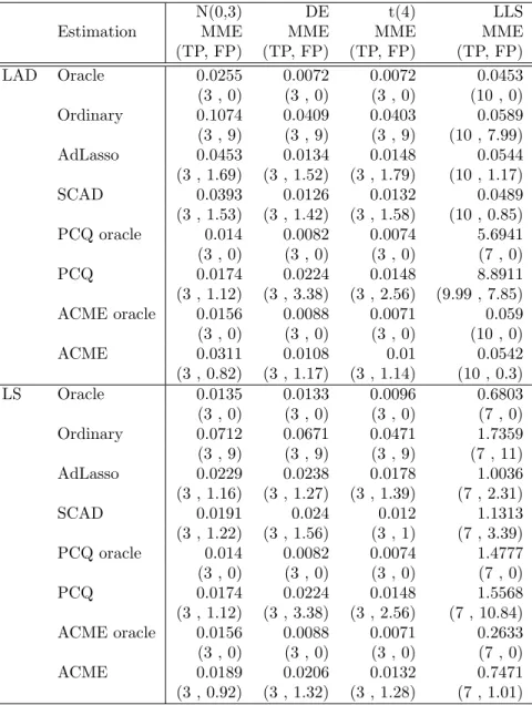
N(0,3) DE t(4) LLS
Estimation MME MME MME MME
(TP, FP) (TP, FP) (TP, FP) (TP, FP)
LAD Oracle 0.0255 0.0072 0.0072 0.0453
(3 , 0) (3 , 0) (3 , 0) (10 , 0)
Ordinary 0.1074 0.0409 0.0403 0.0589
(3 , 9) (3 , 9) (3 , 9) (10 , 7.99)
AdLasso 0.0453 0.0134 0.0148 0.0544
(3 , 1.69) (3 , 1.52) (3 , 1.79) (10 , 1.17)
SCAD 0.0393 0.0126 0.0132 0.0489
(3 , 1.53) (3 , 1.42) (3 , 1.58) (10 , 0.85)
PCQ oracle 0.014 0.0082 0.0074 5.6941
(3 , 0) (3 , 0) (3 , 0) (7 , 0)
PCQ 0.0174 0.0224 0.0148 8.8911
(3 , 1.12) (3 , 3.38) (3 , 2.56) (9.99 , 7.85)
ACME oracle 0.0156 0.0088 0.0071 0.059
(3 , 0) (3 , 0) (3 , 0) (10 , 0)
ACME 0.0311 0.0108 0.01 0.0542
(3 , 0.82) (3 , 1.17) (3 , 1.14) (10 , 0.3)
LS Oracle 0.0135 0.0133 0.0096 0.6803
(3 , 0) (3 , 0) (3 , 0) (7 , 0)
Ordinary 0.0712 0.0671 0.0471 1.7359
(3 , 9) (3 , 9) (3 , 9) (7 , 11)
AdLasso 0.0229 0.0238 0.0178 1.0036
(3 , 1.16) (3 , 1.27) (3 , 1.39) (7 , 2.31)
SCAD 0.0191 0.024 0.012 1.1313
(3 , 1.22) (3 , 1.56) (3 , 1) (7 , 3.39)
PCQ oracle 0.014 0.0082 0.0074 1.4777
(3 , 0) (3 , 0) (3 , 0) (7 , 0)
PCQ 0.0174 0.0224 0.0148 1.5568
(3 , 1.12) (3 , 3.38) (3 , 2.56) (7 , 10.84)
ACME oracle 0.0156 0.0088 0.0071 0.2633
(3 , 0) (3 , 0) (3 , 0) (7 , 0)
ACME 0.0189 0.0206 0.0132 0.7471
(3 , 0.92) (3 , 1.32) (3 , 1.28) (7 , 1.01)
than the ZG ratio. The ZG ratio of ACME is almost 30% higher than that of all
separate estimators under the both n = 100 and n = 500. ACME has almost two thirds NG ratio except for the normal distribution with n= 100. Note that Ordinary, AdLasso, and SCAD have zero NG ratios because the separate estimation does not
involve any overlapping penalization. PCQ possesses complete overlapping because
the dataset is assumed to be generated from a classical linear model. Hence, PCQ
successfully recovers the overlapping structure.
2.4.2 Linear Location-Scale Model
Under linear location-scale models, both LS regression and LAD regression are
partially overlapping models as some covariates affect the scale of the response. Our
dataset is generated from the following linear location-scale model:
yi =xTi β 0
+xTi γ0i,
whereβ0 = (3,3,3,3,3,3,3,0,0,0,0,0,0,0,0,0,0,0)T andγ0 = (0,0,0,0,3,−3,3,−3,3, −3,0,0,0,0,0,0,0,0)T. The covariate, x
i = (xi1, · · · , xi18)T, is generated from a
mul-tivariate standard normal distribution, N(0, I18×18). Assume that the error term, i,
follows a shifted gamma distribution, Γ(0.25, 2)−0.5. Note that the distribution is skewed to the right and centered to mean 0. The true parameter vector of the LS
regression model isβ0ls =β0 and the true parameter vector of LAD regression model is
β0lad = (3,3,3,3,1.762,4.238,1.762,1.238,−1.238,1.238,0,0,0,0,0,0,0,0)T. Similar to Section 2.4.1, we use the composite L1-L2 loss function. We implement the simulation
with 100 repetitions under n = 100 and n= 500.
From the last columns of Tables 2.1 and 2.2, the ACME has the second smallest