All-Resolutions Inference for Brain Imaging
Jonathan D. Rosenblatt
∗Livio Finos
†Wouter D. Weeda
‡Aldo Solari
§Jelle J. Goeman
¶1
Abstract
The most prevalent approach to activation localization in neuroimaging is to identify brain regions as contiguous supra-threshold clusters, check their significance using random field theory, and correct for the multiple clusters being tested. Besides recent criticism on the validity of the random field assumption, a spatial specificity paradox remains: the larger the detected cluster, the less we know about the location of activation within that cluster. This is because cluster inference implies “there exists at least one voxel with an evoked response in the cluster”, and not that “all the voxels in the cluster have an evoked response”. Inference on voxels within selected clusters is considered bad practice, due to the voxel-wise false positive rate inflation associated with this circular inference. Here, we propose a remedy to the spatial specificity paradox. By applying recent results from the multiple testing statistical literature, we are able to quantify the proportion of truly active voxels within selected clusters, an approach we call All-Resolutions Inference (ARI). If this proportion is high, the paradox vanishes. If it is low, we can further “drill down” from the cluster level to sub-regions, and even to individual voxels, in order to pinpoint the origin of the activation. In fact, ARI allows inference on the proportion of activation in all voxel sets, no matter how large or small, however these have been selected, all from the same data. We use two fMRI datasets to demonstrate the non-triviality of the spatial specificity paradox, and its resolution using ARI. One of these datasets is large enough for us to split it and validate the ARI estimates. The conservatism of ARI inference permits circularity without losing error guarantees, while still returning informative estimates.
2
Introduction
The fundamental building block of brain mapping with functional magnetic resonance imaging (fMRI) is arguably the localization of evoked brain responses to cognitive stimuli. Localization is typically performed by correlating a sequence of stimuli to the sequence of measured blood oxygenation levels (BOLD) at each brain region, and then testing for the statistical significance of these correlations. Correlation should be understood in a broad sense, and may involve simple correlations, linear models, non-linear models, machine learning classifiers, and more. A region is declared “active”, or “information-encoding”, if this correlation is statistically significant compared to an “inactive region” null hypothesis. Clearly, testing many regions in the brain introduces a severe multiplicity problem, leading, for example, to the detection of information-encoding regions in dead salmon fish [Bennett et al., 2009]. Error rate inflation was acknowledged by the neuroimaging community early on, and led to an awareness in the community of the dangers ofselective inference. Selective
∗Department of IE&M and Zlotowsky Center for Neuroscience, Ben Gurion University of the Negev, Israel †DPSS, University of Padua, Italy
‡Methodology & Statistics Unit, Department of Psychology, Leiden University, Leiden, The Netherlands, and Leiden Institute for Brain and Cognition, Leiden University, Leiden, The Netherlands
inference includesselective testing, better known asmultiple testing [Friston et al., 1991, Genovese et al., 2002], and alsoselective estimation, better known as voodoo correlations, circular inference, anddouble-dipping [Vul et al., 2009, Kriegeskorte et al., 2009, Rosenblatt and Benjamini, 2014]. The community’s awareness of selective inference is manifested in the fact that all software suites for brain imaging (SPM, FSL, BrainVoyager, and AFNI) include several multiplicity correction methods. It is also manifested in the fact that it is impossible to publish a paper in the field if multiplicity has not been addressed.
The localization of activation in the brain requires the neuroscientist to choose the type of inference to make. This includes (i) the scale of brain regions, and (ii) the choice of error guarantees. The scale of brain regions may vary from a single volume element (voxel), to multiple contiguous elements defined by their shape, their anatomical properties, or their functional properties. These are known asvoxel-wise inference, searchlight,anatomical regions of interest (ROIs), andfunctional regions of interest, respectively. The error guarantee applied is typically thefamily-wise error rate (FWER), or thefalse discovery rate(FDR). FWER is interpretable as the proportion of studies in which false discoveries are made, and FDR as the averagefalse discovery proportionover all studies. Historically, the first inferences were voxel-wise, or anatomical ROIs, with FWER error guarantees. Then came functional ROIs, FDR controls, multivariate searchlights, and others. Today, combinations of all scales of inference with all error controls can be found in the neuroimaging literature [e.g. Poldrack et al., 2011].
A scale of inference which deserves particular attention iscluster-based inference. The idea of cluster inference dates back to Poline and Mazoyer [1993], Forman et al. [1995], and Friston et al. [1996]. It is now the most common type of inference, being the default option in several popular software suites. Cluster inference can be seen as inference at adata-driven scale. This is because the size of the clusters is not selected a priori, but rather determined by the data used for inference. The fact that clusters are both defined and tested with the same data introduces a statistical circularity challenge typically solved using arandom field theory (RFT) approach, which permits both FWER control on clusters [Taylor and Worsley, 2007a], and FDR control on clusters [Chumbley et al., 2010].
Unfortunately, cluster inference has been heavily criticized, firstly for inappropriate error guarantees, as recently shown in the high-profile contribution of Eklund et al. [2016].
Cluster inference also suffers from low spatial resolution [Woo et al., 2014], which is demonstrated by the following paradox. Since discovering a cluster means that “there exists at least one voxel with an evoked response in the cluster”, and not that “all the voxels in the cluster have an evoked response”, it follows thatthe larger the detected cluster, the less information we have on the location of the activation. Moreover, cluster-based inference gives no information on the extent of the activation within the cluster.
The matter of low spatial resolution can be remedied by a hierarchical approach1—a “drill-down” from discovered clusters to subsets of those clusters, and ultimately, to the voxel level. The aim of a drill-down is to localize the activation within the cluster, and to quantify its extent. However, it is typically a forbidden practice, because voxel-wise error guarantees will not hold when inferring on voxels within selected clusters. Such a drill-down would entail three layers of circularity: creating clusters, inferring on clusters, and inferring on voxels within clusters. Acknowledging the three layers of circularity for valid inference is a formidable mathematical challenge. The purpose of this manuscript is to report the application of a recent advance in the hierarchical inference literature, namely that of Goeman and Solari [2011], to permit valid circular inference of this type in neuroimaging.
TheAll-Resolutions Inference (ARI) of Goeman and Solari [2011] allows more than a single drill-down from the cluster to the voxel: it allows the researcher to apply any data-driven region selection and estimate the proportion of true discoveries(PTD2) of any subregion—clusters in our case—all from the same dataset. ARI accounts for the circularity by controlling the FWER over all possible subsets of the brain, large or small, contiguous or non-contiguous, usingclosed testing [Marcus et al., 1976]. Extreme conservatism for FWER control over these exponentially many regions can be avoided, if tests for overlapping regions are highly correlated. ARI exploits the powerful Simes test, which exhibits the necessary correlation structure. The
1Sometimes known asmulti-resolution, orpost hoc.
2Readers familiar with thefalse detection rateliterature, will note thatP T D= 1−F DP, whereF DP is thefalse discovery
Simes test is valid under the assumption of the Simes inequality, which is implied by thepositive regression dependency on subsets condition (PRDS), established for brain maps by Nichols and Hayasaka [2003]. The assumption of the Simes inequality is well-known, since it is also necessary for the FDR-controlling procedure of Benjamini and Hochberg [1995]. The closed testing procedure, in combination with the Simes inequality, guarantees FWER control on all statements made using ARI, which means that with probability at least 95% no region has an overestimated PTD.
In Section 3, we prove that ARI returns lower bounds on the PTD, at all scales simultaneously, and for various selection criteria. Examples include voxels within clusters, voxels within searchlights, anatomical ROIs within functional ROIs, etc. The non-technical reader may want to skip directly to Section 4, where we apply ARI to several datasets. From these we learn that the spatial specificity paradox exists empirically and cannot be ignored. For some datasets and thresholds, clusters consist of mostly active voxels, while for other datasets and thresholds, clusters consist of mostly inactive voxels. For the latter clusters, ARI allows one to look at data-driven subclusters to better pinpoint the location of active voxels.
While not our initial motivation, ARI may also serve for cluster inference, thus replacing the RFT p-values. Since ARI does not rely on RFT, it eschews the inaccuracies of cluster inference recently reported by Eklund et al. [2016], and it avoids the computational burden of resampling-based inference. We elaborate on cluster selection with ARI in Section 5.1.
3
The All-Resolutions Inference Framework
We start with an exposition of the ARI method, the datasets to which it has been applied, and the manner in which it has been applied.
3.1
Overview of the Framework
The brainB is a collection ofmvoxels. We assume that a test statistic for activation has been calculated for
each voxel, which can be converted into a voxel-wisep-value.
Researchers are interested in inference on subsets of the brain. In general, we use the termvoxel set for any subset of the brain, possibly non-contiguous. Special types of voxel sets are regions, clusters, and searchlights. We denoteS= 2B as the collection of all|S|= 2mvoxel sets, where| · |denotes the cardinality of a set. Brain regions are interesting if they contain many truly active voxels. Let the unknown voxel setA⊆B be the set
of alltrulyactive voxels. For any voxel setS∈ S, denote the number of truly active voxelsa(S) =|A∩S|, and their proportion (PTD) byπ(S) =a(S)/|S|.
ARI uses the methods of Goeman and Solari [2011] and Meijer et al. [2016] to construct lower confidence bounds ¯π(S) for the set-wise proportion of active voxels, simultaneously for all possible sets. The (1−α)
lower confidence bound is such that
P(for allS∈ S : ¯π(S)≤π(S))≥1−α. (1)
Simultaneity over all S ∈ S, i.e. the fact that the “for all” statement is inside the probability statement, crucially makes all inference based on ¯π(S) robust against circular selection of sets. With probability at least
1−αthe bound is valid for all S, and therefore for one or more selected S, regardless of how they were
selected. Simultaneity, in turn, implies FWER control over all statements made about the selectedS.
In particular ¯π(S) may also be calculated for sets of one voxel, for which it takes the values 0 or 1. In ARI
the singleton sets for which ¯π(S) = 1 precisely correspond to the voxels rejected by the procedure of Hommel
3.2
Simes Test and Simes Inequality
To derive (1) we start by defining for every voxel setS ∈ S the null hypothesis
HS:a(S) = 0.
HS is the usual null hypothesis for cluster-wise inference: rejectingHS indicates that there is at least one active voxel inS. We test everyHS with the Simes test [Simes, 1986], rejectingHS at levelαif and only if
pS≤α, where
pS = min
1≤i≤|S| |S|
i p(i:S)
andp(i:S)is theith smallestp-value among voxels inS.
The Simes test is valid if P(pS≤α)≤αfor allS for whichHS is true. For the validity of the ARI procedure as a whole, however, we only need this to hold for the setS=B\Aof all non-active voxels, the largest set
for whichHS is true. We assume that
P(pB\A≤α)≤α. (2)
Equation (2), the Simes inequality, is the most important assumption required for ARI. The assumption of the Simes inequality is frequently made in the multiple testing literature, and oft-used procedures such as those of Hommel [1988], Hochberg [1988] and Benjamini and Hochberg [1995] make the same assumption. There is, therefore, much ongoing research on sufficient conditions for the validity of the Simes inequality [Finner et al., 2014]. It has been shown to hold for independent p-values, and under various conditions implying
non-negative correlations betweenp-values, one of which is the PRDS condition. Nichols and Hayasaka [2003]
have shown that PRDS, and therefore the Simes inequality, is valid for brain maps.
3.3
All-Region FWER Control
The tests for the 2mhypothesesH
S,S∈ S, must be corrected for multiple testing. A powerful method for this is closed testing [Marcus et al., 1976]. Intuitively, closed testing means that if a particular configuration of true and false null hypotheses may inflate false-positive rates, then the rates for this configuration should be controlled explicitly, for all possible configurations. Formally, in closed testing a hypothesisHS is rejected if and only ifHI is rejected for allI⊇S. Closed testing controls the FWER at levelαfor allHS,S∈ S, under the simple condition thatHB\Ais a validα-level test, i.e. under the assumption of the Simes inequality. Meijer et al. [2016] have proven that closed testing with Simes tests rejects a hypothesisHS if and only if
min 1≤i≤|S|
h ip(i:S)
≤α (3)
where
h= maxi∈ {0, . . . , m}:ip(m−i+j:B)> jα, forj= 1, . . . , i .
Note thathdepends onαand on thep-values of voxels outsideS. Closed testing is a very powerful procedure,
3.4
Proportion of Truly Active Voxels (PTD)
Lower confidence bounds for the percentage of truly active voxels (PTD above) follow from the result of the closed testing procedure by the argument given by Goeman and Solari [2011]: specifically, if for somek≥0,
HI is false for all subsetsI⊆S with|I|=|S| −k, then there is at least one active voxel in each such I, and therefore there are at leastk+ 1 active voxels inS. Goeman and Solari [2011] defined ¯a(S) =|S| − |I|, where
I is the largest subset ofS such thatHI was not rejected by the closed testing procedure.
That ¯a(S) is a simultaneous lower bound on the PTD of the region, i.e. that
P(¯a(S)≤a(S) for allS∈ S)≥1−α,
follows immediately from the FWER-control of the closed testing procedure, and (1) follows immediately by setting ¯π(S) = ¯a(S)/|S|.
For the case of Simes tests, we have
¯
a(S) = minn0≤k≤ |S|: min 1≤i≤|S|−k
h
ip(i+k:S)> α
o
.
Efficient ways to calculate this quantity are given by Meijer et al. [2016]. The lower bound is the minimum number ofp-values that can be removed so that (3) is violated for the resulting subset.
We note that by the properties of closed testing ¯a(S) never increases when drilling down, i.e. reducingS to a
subset. ¯π(S), however, may increase when drilling down unless ¯π(S) = 0. It may pay to drill down for PTD,
but never for regions where no signal is found.
3.5
Image Analysis Pipeline
ARI brings unprecedented freedom in looking at the data, choosing regions in any desired way, calculating PTDs for the chosen regions, and possibly reconsidering the selection, e.g. if regions are too small or too large, or have a disappointingly low percentages of active voxels. Different criteria may be used to select different regions. FWER control is guaranteed as long as theα-level and the method of calculatingp-values
have been decided before seeing the data.
To demonstrate the spatial specificity paradox, and its resolution with ARI, we start by selecting clusters with a standard analysis pipeline, and then compute PTDs in these clusters. Given a Z-score map, we defined clusters of interest using pre-specified cluster-formingZ-threshold and minimal cluster size. The cluster size
threshold we use is equivalent to an RFT significance threshold. The latter choice is only for conforming to current practice. We emphasize that ARI estimates do not rely, in any way, on RFT inference. RFT significance and ARI significance do not necessarily coincide: there may be regions significant under RFT but not under ARI, and vice versa.
To pinpoint activation within these clusters, we drilled down to smaller regions by increasing the cluster-forming threshold toZ >4 and looking at the clusters, significant by RFT or not, that are contained within
the significant clusters atZ >3.2.
The cluster-forming thresholds of 3.2 and 4 are arbitrary, and we did not fix them before seeing the data. In
ARI this post hoc choice of regions, and the manner in which they are selected, does not invalidate FWER control for inference on the chosen regions.
For convenience, we collect our two selection criteria as used in this manuscript: 1. Z >3.2 clusters with a size/significance threshold.
3.6
fMRI Data
To demonstrate the results of ARI, we applied it on two fMRI datasets we termGo/No-go, andAuditory. The Go/No-go dataset consists of 34 subjects performing an emotional go/no-go task [Lee et al., under review]. Participants had to press a button when presented with faces with a certain emotional expression (go condition), and withhold their response to faces with a neutral expression (no-go condition). The go and no-go conditions were then reversed, to avoid confounding with button-press-related activation. The Auditory dataset was collected by Pernet et al. [2015], and generously shared via the OpenfMRI initiative at https://openfmri.org/. It consists of 218 subjects passively listening to vocal (i.e. speech) and non-vocal sounds. The large dataset allowed us to validate our PTD estimates on different subjects. We used two mutually exclusive sets, an original sample with a typical fMRI sample size of 33 subjects, and a validation sample of 66 subjects, serving as a “ground-truth”. We used only 66 and not the 185 = 218−33 remaining subjects, so that the “ground-truth” is not driven by infinitesimally small effects.
4
Results
4.1
Go/No-go Data
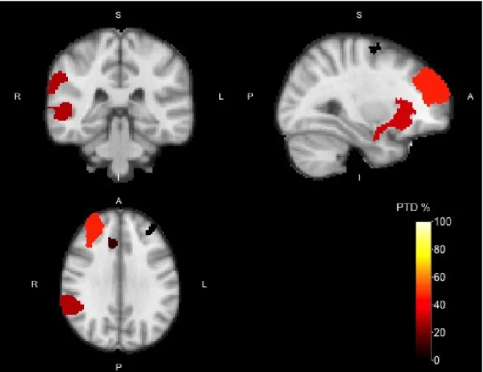
Group analysis of the No-go >Go contrast highlighted 11 regions of interest commonly found in studies
using the Go/No-go paradigm (see Figure 1).
These regions included the left and right insular cortex (IC) extending into the frontal orbital cortex (FOC), the left and right frontal pole (FP), the right middle (MTG) and superior temporal gyrus (STG) extending into the angular gyrus (AG), the right (para)cingular gyrus (PCG), right superior frontal gyrus (SFG), right precuneus, and the right precentral gyrus.
PTDs for these ROIs were highest for the region spanning the right MTG, STG and angular gyrus (2191 voxels, PTD = 28.5%), the region spanning the right frontal pole (1845 voxels, PTD = 46.2%), and the
region spanning the right insular cortex and frontal orbital cortex (1400 voxels, PTD = 32.4%). The regions
spanning the left insular cortex and frontal orbital cortex (421 voxels, PTD = 5.9%), and (para)cingular gyrus
(304 voxels, PTD = 10.9%) had lower PTDs, while for the other regions (right SFG, precuneus, precentral
gyrus, and left frontal pole) the PTD was 0%.
Of the regions with a PTD of 0%, which are not expected to have many active voxels, all four regions had significant RFT-correctedp-values: The right SFG (698 voxels, RFTp < .001, ARIp=.068, PTD = 0%),
right precuneus (245 voxels, RFTp=.010, ARIp=.533, PTD = 0 %), right precentral gyrus (232 voxels,
RFTp=.012, ARIp=.069, PTD = 0%), and left FP (698 voxels, RFT p=.029, ARIp=.497, PTD =
0%).
Details of the clusters can be found in Table 1. Details include the name and size of the clusters, ARI-estimated number and proportion of active voxels, and ARIp-value. In addition we includestandard details on the location of the cluster maximum (MNI coordinates),Z-value of the maximum and RFT-corrected p-values
for each cluster.
To pinpoint the location of the truly active voxels, i.e. to “drill down”, we could infer on all the voxels in selected clusters. ARI guarantees that this inference would be valid but, alas, low-powered. Alternatively, we may increase the cluster-forming threshold. Inference would still be valid, and the PTD would increase, until all supra-threshold voxels are truly active.
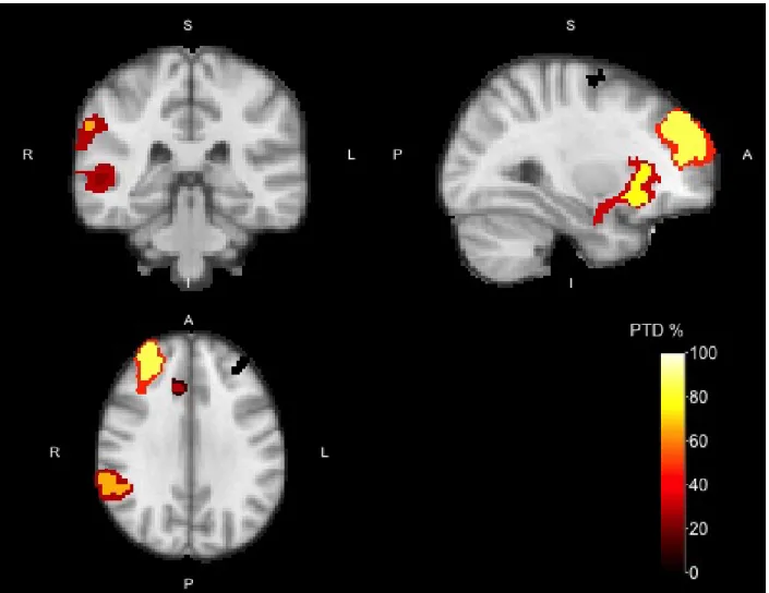
Using a cluster-forming threshold of Z >4 and looking at these “drill down” clusters within the Z >3.2
Figure 1: Activation map of the No-go > Go contrast with cluster-forming thresholdZ >3.2 for the Go/No-go
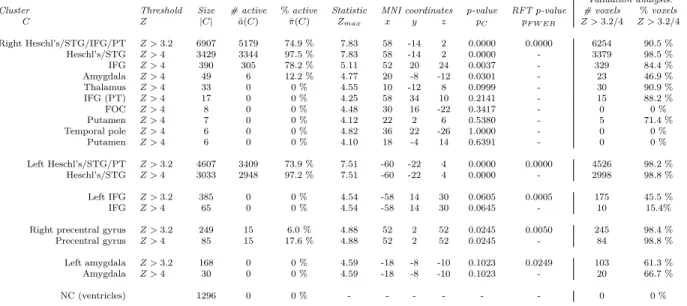
Table 1: Go/No-go data: clusters identified with threshold Z >3.2 (RFTp < .05, cluster size = 161), with
"drill down" clusters atZ >4.
Cluster Threshold Size # active %active Statistic MNI coordinates p-value RFTp-value
C Z |C| ¯a(C) π¯(C) Zmax x y z pC pF W ER
Right MTG, STG, angular gyrus Z >3.2 2191 624 28.5 % 5.25 50 -26 -6 0.0068 0.0000 STG, angular gyrus Z >4 405 267 65.9 % 5.19 68 -40 24 0.0136
-MTG Z >4 133 31 23.3 % 5.25 50 -26 -6 0.0080
-MTG (TO) Z >4 6 0 0 % 4.21 66 -58 10 0.8178
-Right frontal pole Z >3.2 1835 847 46.2 % 5.85 30 46 38 0.0002 0.0000 Z >4 963 826 85.8 % 5.85 30 46 38 0.0002
-Right insular cortex, FOC Z >3.2 1400 454 32.4 % 6.01 32 20 -10 0.0001 0.0000 Insular cortex, FOC Z >4 583 449 77.0 % 6.01 32 20 -10 0.0001
-Amygdala Z >4 4 0 0 % 4.11 20 -4 -12 1.0000
-Amygdala Z >4 1 0 0 % 4.05 30 2 -14 1.0000
-Right SFG Z >3.2 698 0 0 % 4.66 20 0 68 0.0680 0.0000
SFG Z >4 69 0 0 % 4.66 20 0 68 0.0847
-SFG Z >4 13 0 0 % 4.50 14 10 62 0.2749
-SFG Z >4 1 0 0 % 4.03 8 20 66 1.0000
-Left insular cortex, FOC Z >3.2 421 25 5.9 % 5.00 -32 28 0 0.0182 0.0001 Insular cortex, FOC Z >4 84 20 23.8 % 5.00 -32 28 0 0.0194
-FOC Z >4 22 0 0 % 4.79 -28 20 -12 0.1414
-Right (para)cingular gyrus Z >3.2 304 33 10.9 % 4.92 8 22 40 0.0164 0.0034
Z >4 117 33 28.2 % 4.92 8 22 40 0.0164
-Right precuneus Z >3.2 245 0 0 % 3.74 10 -66 44 0.5325 0.0097
Z >4 0 - - -
-Right precentral gyrus Z >3.2 232 0 0 % 4.68 44 0 42 0.0692 0.0123
Z >4 42 0 0 % 4.68 44 0 42 0.0692
-Left frontal pole Z >3.2 187 0 0 % 4.20 -36 54 22 0.4971 0.0291
Z >4 5 0 0 % 4.20 -36 54 22 0.9880
-(STG/AG) are often found in inhibition studies, while the chance of finding a cluster in the MTG is much smaller.
The right FP contained only one smaller cluster (963 voxels, PTD = 85.8%) with a high PTD. The region spanning the right IC and FOC also was divided into three subclusters: one spanning the IC and FOC (583 voxels, PTD = 77.0%) and two spanning the amygdala (1 and 4 voxels respectively, PTD = 0%). The left IC/FOC cluster contained two small clusters, one spanning the IC/FOC (84 voxels, PTD = 23.8%) and one spanning only the FOC (22 voxels, PTD = 0%). Again, these results are consistent with the literature regarding inhibition studies, where the IC/FOC cluster is more often found than the FOC cluster (Neurosynth meta-analysis [Yarkoni et al., 2011], keyword ‘nogo’).
The right PCG contained one small cluster (117 voxels, PTD = 28.2%). For the right SFG, drilling down revealed three clusters all within the SFG (69, 13, and 1 voxel), all with a PTD of 0%. The other regions contained no active voxels in the smaller regions.
The ARI drill-down analysis is thus consistent, and more informative about the smaller clusters. As evident from the drill-down analysis, the new smaller region in the right FP has a higher PTD (85.8% vs 46.2%),
indicating that this smaller area contains most relevant information. The same holds for the right IC/FOC (32.4% vs 77.0%) and STG/AG areas (28.2% vs 65.9%), where the new smaller regions now contain a more
Figure 2: Activation map of the No-go > Go contrast with cluster-forming thresholdZ >4 for the Go/No-go
4.2
Auditory Data
4.2.1 Inference
Group analysis on the first set of 33 subjects of the Vocal>Non-vocal contrast showed activity in 6 regions
of interest commonly found in auditory studies. Details of the clusters can be found in Table 2. We observed activity bilaterally in the superior temporal gyrus (STG), planum temporale (PT), Heschl’s gyrus (HG), inferior frontal gyrus (IFG), and amgydala, and activity in the right precentral gyrus.
Table 2: Auditory data: clusters identified with thresholdZ >3.2 (RFTp < .05, cluster size = 118), with
"drill down" clusters atZ >4.
Validation analysis: Cluster Threshold Size # active %active Statistic MNI coordinates p-value RFTp-value # voxels %voxels
C Z |C| ¯a(C) ¯π(C) Zmax x y z pC pF W ER Z >3.2/4 Z >3.2/4
Right Heschl’s/STG/IFG/PT Z >3.2 6907 5179 74.9 % 7.83 58 -14 2 0.0000 0.0000 6254 90.5 %
Heschl’s/STG Z >4 3429 3344 97.5 % 7.83 58 -14 2 0.0000 - 3379 98.5 %
IFG Z >4 390 305 78.2 % 5.11 52 20 24 0.0037 - 329 84.4 %
Amygdala Z >4 49 6 12.2 % 4.77 20 -8 -12 0.0301 - 23 46.9 %
Thalamus Z >4 33 0 0 % 4.55 10 -12 8 0.0999 - 30 90.9 %
IFG (PT) Z >4 17 0 0 % 4.25 58 34 10 0.2141 - 15 88.2 %
FOC Z >4 8 0 0 % 4.48 30 16 -22 0.3417 - 0 0 %
Putamen Z >4 7 0 0 % 4.12 22 2 6 0.5380 - 5 71.4 %
Temporal pole Z >4 6 0 0 % 4.82 36 22 -26 1.0000 - 0 0 %
Putamen Z >4 6 0 0 % 4.10 18 -4 14 0.6391 - 0 0 %
Left Heschl’s/STG/PT Z >3.2 4607 3409 73.9 % 7.51 -60 -22 4 0.0000 0.0000 4526 98.2 %
Heschl’s/STG Z >4 3033 2948 97.2 % 7.51 -60 -22 4 0.0000 - 2998 98.8 %
Left IFG Z >3.2 385 0 0 % 4.54 -58 14 30 0.0605 0.0005 175 45.5 %
IFG Z >4 65 0 0 % 4.54 -58 14 30 0.0645 - 10 15.4%
Right precentral gyrus Z >3.2 249 15 6.0 % 4.88 52 2 52 0.0245 0.0050 245 98.4 %
Precentral gyrus Z >4 85 15 17.6 % 4.88 52 2 52 0.0245 - 84 98.8 %
Left amygdala Z >3.2 168 0 0 % 4.59 -18 -8 -10 0.1023 0.0249 103 61.3 %
Amygdala Z >4 30 0 0 % 4.59 -18 -8 -10 0.1023 - 20 66.7 %
NC (ventricles) 1296 0 0 % - - - 0 0 %
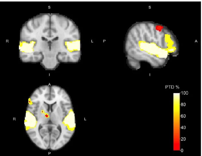
As can be seen in Figure 3, the activity in the right hemisphere covered one large cluster (6907 voxels), with a PTD of 74.9% (with exception of the precentral gyrus; 249 voxels, PTD = 6.0%). In the left hemisphere
these same areas were divided amongst three regions: HG/STG/PT (4607 voxels, PTD = 73.9%), IFG (385
voxels, PTD = 0%), and the amygdala (168 voxels, PTD = 0%).
As with the previous analysis we can now drill down with a higher cluster-forming threshold to check the proportion of active voxels in the smaller regions. With a cluster-forming threshold ofZ >4, we now see 15
smaller regions within theZ >3.2 clusters (see Figure 4). The large cluster in the right hemisphere of the
temporal cortex in theZ >3.2 analysis now separates into 9 separate clusters. Three of these clusters had
a PTD larger than 0%: HG/STG (3429 voxels, PTD =97.5%), IFG (390 voxels, PTD = 78.2%), and the amygdala (49 voxels, PTD = 12.2%); the other clusters contained no active voxels (see Table 2 for details). The HG/STG cluster in the left hemisphere was now also smaller, with a high PTD (3033 voxels, PTD = 97.2%). The smaller clusters in the left amygdala, and IFG, contained no active voxels (PTD = 0%). The smaller cluster in the right precentral gyrus (85 voxels, PTD = 17.6%), had a slightly higher PTD value.
4.2.2 Validation
To check the validity of the ARI method we used theZ >3.2 andZ >4 clusters from the previous analysis
and calculated the number of supra-threshold voxels of these clusters using data from the second set of 66 subjects. The following results confirms that the ARI PTD bounds are both informative and statistically valid, despite the circular analysis.
ForZ >3.2, the validation dataset showed 90.5% supra-threshold voxels in the right Heschl’s gyrus/STG,
Figure 3: Activation map of the Vocal > Non-vocal contrast with cluster-forming thresholdZ >3.2 for the
Figure 4: Activation map of the Vocal > Non-vocal contrast with cluster-forming thresholdZ >4 for the
supra-threshold voxels, compared to a PTD of 73.9% in the original sample. In the left IFG the number of
supra-threshold voxels was 45.5%, compared to a PTD of 0% in the original sample. The right precentral
gyrus showed 98.4% supra-threshold voxels, compared to a PTD of 6.0% in the original sample. In the left
amygdala we observed 61.3% supra-threshold voxels, with a PTD of 0% in the original sample. The negative
control region (NC; left/right ventricles) showed no significant supra-threshold voxels.
5
Discussion
We set out to improve the spatial specificity of detected regions using a “drill-down” approach—first selecting clusters, and then inferring on the voxels in those selected clusters—all with the same data. Reporting the proportion of active voxels in a cluster is an old quest in neuroimaging [e.g. Turkheimer et al., 2001], which also fulfills recent recommendations to report effect sizes, and not only active/inactive areas or cluster
p-values [APA, 2001, Wilkinson, 1999].
Concerned with error inflation after the drill-down, we define an error to be an over-estimation of the proportion of truly active voxels in a region. Put differently, we are able to estimate the proportion of truly active voxels (PTD) in a selected cluster, with FWER control over clusters, all from the same data. This is made possible using results from Goeman and Solari [2011]. The fundamental observation is that if a statistical parametric map (SPM) of the brain satisfies the Simes inequality, then inferring on all possible voxel subsets is not hopelessly under-powered. Clearly, voxels within selected clusters are a subset of all voxel subsets, so that inference remains valid, for all possible subsets: in particular, for all the ones the practitioner queries after seeing the data.
Readers familiar with Scheffé’s post hoc test [Scheffe, 1953], may recognize that we use the same type of statistical reasoning. By controlling the error rate for all possible contrasts, Scheffé’s test allows the practitioner to choose the contrast after seeing the data. ARI does the same, not for all possible contrasts, but for all possible set selections. Moreover, and unlike Scheffé, ARI uses closed testing, which is more powerful in this context.
Quantifying the amount of true signal within clusters allows us to address the “spatial specificity paradox”, whereby the larger a cluster the less we know about the location of the signal. If the proportion of truly active voxels in a cluster is large, there is no real paradox. If this proportion is small, the practitioner should consider reducing the size of the clusters. Our two datasets demonstrate this is not a mere philosophical discussion, but rather, an empirical question with very real implications. The Go/No-go dataset shows small proportions of true activation within clusters, so that it is hard to tell which part of the cluster is truly active. The Auditory data shows large proportions, implying that the clusters are indeed mostly active.
The validation analysis shows consistent results across the two datasets: regions with a high PTD tend to have a high percentage of supra-threshold voxels in the validation dataset, and vice-versa. The PTD bounds are informative, i.e. not overly conservative, provided that the region is large enough: the gap between the PTD bound and the validated activation proportion is not too large. Smaller regions suffer a larger multiple testing burden, and so are more difficult to detect using ARI. The power of ARI is better for large clusters than for smaller ones, and better for small clusters than for single voxels. As a result it is easier to detect the presence of active voxels than it is to pinpoint them. A region may have a large proportion of active voxels, but we cannot usually say which voxels these are. This is especially true if the signal in a region is dispersed. In that case drilling down may not be successful: there may not always be a subregion with evidence for a larger PTD.
region for which one is confident of a PTD of at least 0.7. While exploring the brain, computation time is not
an issue. The underlying computations have been implemented in the R packagehommel [Goeman et al., 2017], and take seconds to perform fromp-value maps.
Our proofs assume the brain’s SPM satisfies the Simes inequality, while many analysis suites use a random field assumption (RFT) [Taylor and Worsley, 2007b]. The criticism of the validity of cluster inference voiced by Eklund et al. [2016] targets the RFT. We adopt the Simes inequality assumption because it facilitates our proofs, but it also means that if the ARI framework is used for cluster selection, it will not be subject to that criticism. The Simes inequality which we use instead of the RFT is implied by the PRDS condition, which has been established for brain SPMs by Nichols and Hayasaka [2003]. It may be possible to use RFT in combination with closed testing to obtain alternative lower bounds for PTD, but this is beyond the scope of this paper.
5.1
ARI for Cluster Selection
Our main innovation is in replacing the problem of cluster selection, with the problme ofP T D-estimation.
Cluster selection (i.e. testing) only claims that PTD >0 for its regions, while ARI claims a non-trivial
lower bound to PTD. Can ARI be used for the cluster selection itself? The answer is affirmative. The practitioner may toggle the cluster-wise cluster-forming threshold until reaching the desired PTD. E.g., select clusters with more than 70% of activation. Alternatively, the user may ask which clusters are the most active, i.e. where the activation is concentrated. Intuitively, the practitioner may “grow clusters”, i.e. decrease the cluster-forming threshold. At some point, the PTD will start to sharply decrease, and the practitioner would then stop growing the clusters. Theconcentration set in Meijer et al. [2016] formalizes this process. It gives a data-dependentp-value threshold above which ARI detects no signal. Used as a cluster-forming threshold,
this gives a useful starting point from which to start the drill-down.
When using ARI for cluster selection, the question of power immediately arises. Naturally, the power properties of ARI are different to those of RFT-based models because the assumptions underlying the methods are different. RFT-selected clusters are not guaranteed to haveP T D >0 in ARI. However, such
a comparison is not completely fair, as RFT-based methods only inferP T D >0 on a limited number of
clusters, while ARI infers the actual value of PTD on exponentially many clusters. Put differently, if a researcher only wishes to demonstrateP T D >0 at a pre-chosen threshold, RFT based methods may be more
powerful. If the researcher varies the cluster-forming threshold, focuses on sub-clusters, or wants to quantify the PTD, this is only possible with ARI.
Comparing power to other multiple testing procedures, we can say that ARI is strictly more powerful than voxel-wise FWER control. It guaranteesP T D >0 for every region containing a Bonferroni-significant voxel.
For large regions it tends to give much larger values of PTD than would result from voxel-wise FWER. A comparison of ARI to FDR-based methods is more complex because FDR is a much more relaxed criterion than FWER. Regarding voxel-wise FDR control, it holds that whenever the Benjamini-Hochberg algorithm [Benjamini and Hochberg, 1995] detects at least one active voxel, ARI will find at least one region with
P T D >0. Direct comparison with cluster-wise FDR is impossible, especially since there is at this moment
no method that controls FDR over all clusters as ARI does.
6
Methods
6.1
Preprocessing
width at half maximum), and registered to standard space using linear registration (FLIRT [Jenkinson and Smith, 2001, Jenkinson et al., 2002] with 12 degree-of-freedom boundary-based registration). Six motion regressors (MCFLIRT [Jenkinson et al., 2002]) and periods with excessive motion were modeled as additional confound regressors. Boxcar functions of the stimulus timings for the different conditions were convolved with a double-gamma hemodynamic response function, with a temporal derivative to model differences in slice acquisition time. For the Go/No-go dataset we analyzed the No-go>Go contrast using FEAT [Woolrich
et al., 2001], using FLAME 1 estimation with a cluster-threshold multiple comparison correction based on RFT, highlighting brain regions involved in successfully inhibiting a response. For the auditory dataset we analyzed the Vocal>Non-vocal contrast, highlighting brain regions involved in speech processing.
ARI was performed on both our datasets using our own implementation, made publicly available in the hommelpackage [Goeman et al., 2017] for theRsoftware environment [Team, 2000]. We used the analysis
pipeline described in Section 3.5.
6.2
ARI Validation
If the PTD of a cluster is bounded byq, then in a new dataset, a proportion of at leastqof the voxels in the
cluster are true signal, and thus should be rediscovered. To validate that this is indeed the case, we used the clusters from the Vocal>Non-vocal contrast of the first set of 33 subjects, and computed the proportion of
supra-threshold voxels (uncorrectedp-value< .05) in a new set of 66 subjects.
Table 2 for the Auditory dataset therefore includes additional columns for the number and percentage of suprathreshold voxels in the verification dataset. In addition, we calculated the PTD in a negative control region where we don’t expect any significant voxels. We used the left and right ventricles (Harvard–Oxford atlas with a probability threshold>50%), and calculated the PTD in each of these areas for both Auditory
datasets.
Bibliography
APA. Publication Manual of the American Psychological Association. American Psychological Association Washington DC, 2001.
Y. Benjamini and Y. Hochberg. Controlling the false discovery rate: A practical and powerful approach to
multiple testing. JOURNAL-ROYAL STATISTICAL SOCIETY SERIES B, 57:289–289, 1995.
C. M. Bennett, M. B. Miller, and G. L. Wolford. Neural correlates of interspecies perspective taking in the post-mortem Atlantic Salmon: An argument for multiple comparisons correction. Neuroimage, 47(Suppl 1):S125, 2009.
J. Chumbley, K. Worsley, G. Flandin, and K. Friston. Topological FDR for neuroimaging. NeuroImage, 49 (4):3057–3064, 2010. ISSN 1053-8119.
A. Eklund, T. E. Nichols, and H. Knutsson. Cluster failure: Why fMRI inferences for spatial extent have inflated false-positive rates. Proceedings of the National Academy of Sciences, 113(28):7900–7905, Dec. 2016. ISSN 0027-8424, 1091-6490.
H. Finner, M. Roters, and K. Strassburger. On the Simes test under dependence. Statistical Papers, pages 1–15, 2014.
K. J. Friston, C. D. Frith, P. F. Liddle, and R. S. J. Frackowiak. Comparing Functional (PET) Images: The Assessment of Significant Change. Journal of Cerebral Blood Flow and Metabolism: Official Journal of the International Society of Cerebral Blood Flow and Metabolism, 11(4):690–699, July 1991. ISSN 0271-678X.
K. J. Friston, A. Holmes, J.-B. Poline, C. J. Price, and C. D. Frith. Detecting Activations in PET and fMRI: Levels of Inference and Power. NeuroImage, 4(3):223–235, Dec. 1996. ISSN 1053-8119.
C. R. Genovese, N. A. Lazar, and T. Nichols. Thresholding of statistical maps in functional neuroimaging using the false discovery rate. NeuroImage, 15(4):870–8, Apr. 2002. ISSN 1053-8119.
J. Goeman, R. Meijer, and T. Krebs. hommel: Methods for Closed Testing with Simes Inequality, in Particular Hommel’s Method, 2017. R package version 1.1.
J. J. Goeman and A. Solari. Multiple Testing for Exploratory Research. Statistical Science, 26(4):584–597, 2011. ISSN 0883-4237.
Y. Hochberg. A sharper Bonferroni procedure for multiple tests of significance. Biometrika, 75(4):800–802, 1988.
G. Hommel. A stagewise rejective multiple test procedure based on a modified Bonferroni test. Biometrika, 75(2):383–386, 1988.
M. Jenkinson and S. Smith. A global optimisation method for robust affine registration of brain images. Medical Image Analysis, 5(2):143–156, 2001. ISSN 13618415.
M. Jenkinson, P. Bannister, M. Brady, and S. Smith. Improved optimisation for the robust and accurate linear registration and motion correction of brain images. NeuroImage, 17(2):825–841, 2002. ISSN 10538119. M. Jenkinson, C. F. Beckmann, T. E. Behrens, M. W. Woolrich, and S. M. Smith. Fsl. Neuroimage, 62(2):
782–790, 2012.
N. Kriegeskorte, W. K. Simmons, P. S. F. Bellgowan, and C. I. Baker. Circular analysis in systems neuroscience: The dangers of double dipping. Nature Neuroscience, 12(5):535–540, May 2009. ISSN 1097-6256.
N. Lee, W. Weeda, C. Insel, L. Somerville, L. Krabbendam, and M. Huizinga. Neural substrates of the influence of emotional cues on cognitive control in risk-taking adolescents. under review.
R. Marcus, E. Peritz, and K. Gabriel. Closed testing procedures with special reference to ordered analysis of variance. Biometrika, 63(3):655–660, 1976. ISSN 0006-3444.
R. Meijer, T. Krebs, A. Solari, and J. Goeman. Simultaneous control of all false discovery proportions by an extension of hommel’s method. arXiv preprint arXiv:1611.06739, 2016.
T. Nichols and S. Hayasaka. Controlling the familywise error rate in functional neuroimaging: A comparative review. Statistical Methods in Medical Research, 12(5):419–446, Jan. 2003. ISSN 0962-2802, 1477-0334. C. R. Pernet, P. McAleer, M. Latinus, K. J. Gorgolewski, I. Charest, P. E. G. Bestelmeyer, R. H. Watson,
D. Fleming, F. Crabbe, M. Valdes-Sosa, and P. Belin. The human voice areas: Spatial organization and inter-individual variability in temporal and extra-temporal cortices. NeuroImage, 119:164–174, Oct. 2015. ISSN 1053-8119.
R. Poldrack, J. Mumford, and T. Nichols. Handbook of Functional MRI Data Analysis. Cambridge University Press, 1 edition, Aug. 2011. ISBN 0-521-51766-4.
J. B. Poline and B. M. Mazoyer. Analysis of individual positron emission tomography activation maps by detection of high signal-to-noise-ratio pixel clusters. Journal of Cerebral Blood Flow and Metabolism: Official Journal of the International Society of Cerebral Blood Flow and Metabolism, 13(3):425–437, May 1993. ISSN 0271-678X.
H. Scheffe. A method for judging all contrasts in the analysis of variance. Biometrika, pages 87–104, 1953. R. J. Simes. An Improved Bonferroni Procedure for Multiple Tests of Significance. Biometrika, 73(3):751–754,
Dec. 1986. ISSN 00063444. ArticleType: primary_article / Full publication date: Dec., 1986 / Copyright © 1986 Biometrika Trust.
S. M. Smith. Fast robust automated brain extraction. Human Brain Mapping, 17(3):143–155, 2002. ISSN 10659471.
J. Taylor and K. Worsley. Detecting Sparse Signals in Random Fields, With an Application to Brain Mapping. Journal of the American Statistical Association, 102(479):913–928, Sept. 2007a. ISSN 0162-1459, 1537-274X.
J. E. Taylor and K. J. Worsley. Detecting sparse signals in random fields, with an application to brain mapping. Journal of the American Statistical Association, 102(479):913–928, 2007b.
R. C. Team. R language definition. Vienna, Austria: R foundation for statistical computing, 2000.
F. E. Turkheimer, C. B. Smith, and K. Schmidt. Estimation of the Number of “True” Null Hypotheses in Multivariate Analysis of Neuroimaging Data. NeuroImage, 13(5):920–930, May 2001. ISSN 1053-8119. E. Vul, C. Harris, P. Winkielman, and H. Pashler. Puzzlingly High Correlations in fMRI Studies of Emotion,
Personality, and Social Cognition. Perspectives on Psychological Science, 4(3):274–290, May 2009. ISSN 1745-6916, 1745-6924.
L. Wilkinson. Statistical methods in psychology journals: Guidelines and explanations.American Psychologist, 54(8):594–604, 1999. ISSN 1935-990X(Electronic);0003-066X(Print).
C.-W. Woo, A. Krishnan, and T. D. Wager. Cluster-extent based thresholding in fmri analyses: pitfalls and recommendations. Neuroimage, 91:412–419, 2014.
M. W. Woolrich, B. D. Ripley, M. Brady, and S. M. Smith. Temporal Autocorrelation in Univariate Linear Modeling of FMRI Data. NeuroImage, 14(6):1370–1386, 2001. ISSN 10538119.