ON THE VOLUME FROM PLANAR SECTIONS THROUGH A CURVE
X
IMOG
UAL-A
RNAUDepartment of Mathematics,Campus Riu Sec, s/n,University Jaume I,12071-Castell´o,Spain e-mail: [email protected]
(Accepted October 19, 2004)
ABSTRACT
We derive a formula to obtain the volume of a compact domain from planar sections through a curve. From this formula we propose a stereological estimator for the volume which generalizes some known unbiased estimators which use a systematic sampling scheme. Moreover we formulate a Cavalieri’s principle for compact domains is spaces of constant curvatureλ.
Keywords: Cavalieri, curve, planar sections, space form, unbiased estimator, volume.
INTRODUCTION
A problem of biomedical interest is how to estimate the volume of an object (bladder, prostate, ...) from planar sections. The best known method to obtain an unbiased estimation of this volume is provided by the Cavalieri’s principle, which is based on parallel equidistant plane sections; that is, orthogonal plane sections through a line. The Cavalieri’s method has been used for scanning techniques such as computed tomography (Pacheet al., 1993) or magnetic resonance imaging (Robertset al., 1994). However, it is difficult to obtain parallel sections of a given object (organ) by ultrasound scan when such obstacles as bones or air are present between the scanner and the organ. In this case, in Watanabe (1982) the volume of an object inR3is calculated from planar sections through a curve of centroids. From this result, a numerical method has been developed to approximate the volume of an object, whose accuracy has been proved in Treece et al. (1999). However, an unbiased estimator of the volume is not available from this method and only from scanning planes which emanate from a common axis, an unbiased estimator for the volume has been derived, based on the ancient theorem of Pappus of Alexandria (Cruz-Orive and Roberts, 1993).
Here we calculate the volume of a compact domain inRnfrom plane sections through a curvec(t). When c(t) is a line and the plane sections are orthogonal to the curve we obtain the Cavalieri method; when c(t) is a curve of centroids of the plane sections we obtain the formula in Watanabe (1982) and whenc(t) is a circumference and the plane sections are normal to c(t), these plane sections are rotating planes that contain a vertical axis and we have the result in Cruz-Orive and Roberts (1993). Moreover, from this formula we obtain an unbiased estimator for the volume when systematic sampling through the curve is considered.
Stereological estimators of volume, using a systematic sampling scheme, are usually much more precise than those based on independent sampling. Therefore, systematic sampling is widely used in stereology as sampling scheme. Here we will consider systematic sampling through a curve to obtain unbiased estimators for the volume.
Since our principal aim is to present the mathematical foundations to derive formulas to calculate the volume from plane sections through a curve, in section “Volume of domains in Rn” we derive the general formula for domains inRn and we obtain some important consequences of this formula. However, in section “Stereological applications” we will concentrate on the applications in volume and area estimation inR3andR2, respectively, and we add two examples of bodies with sectional planes orthogonal to different curves. In section “Discussion” we generalize some results for compact domains in a space form Mn
λ of dimensionnand sectional curvatureλ, and we formulate a Cavalieri’s principle inMn
λ.
VOLUME OF DOMAINS IN
R
nLetDbe a compact domain in then-dimensional euclidean space Rn. Let c : I = [0,L] −→ Rn be a C∞ curve parametrized by its arc-length t (c(t) may be inside D or not). For every t ∈ I, let Pt denote a (n−1)-dimensional plane (hyperplane) in Rn through c(t) (not necessarily orthogonal to c(t)). Let {E1(t),E2(t), . . . ,En(t)} be a smooth orthonormal frame alongc(t)such that, for eacht∈I, {E2(t),E3(t), . . . ,En(t)}is a basis ofTc(t)Pt ≡Pt.
From now on we will suppose that there exist subsetsDt ⊂Pt∩Dsuch that
D=[ t I
Under the above hypotheses, each pointxt∈Dt will be given as
xt=c(t) + n
∑
i=2
µi(t)Ei(t). (2)
Let µ(t) = ∑ni=2µi(t)Ei(t) = ∑ni=2hµ(t),Ei(t)iEi(t) andN(t) =µ(t)/|µ(t)|; then,
xt=c(t) +rtN(t), (3)
wherert=dist(c(t),xt).
Theorem 1.The volume ofDis given by
Voln(D) =
Z L
0 Voln−1(Dt)hc
0(t),E1(t)idt
− Z L
0
Z
Dt
rthN(t),dtd E1(t)iσtdt, (4)
whereσt is the(n−1)-dimensional volume element of
Pt.
Proof. Let ω be the volume element in Rn and we consider on D the coordinates given by (t,µ2(t), . . . ,µn(t)); then,
Voln(D) =
Z
Dω=
Z L
0
Z
Dt
ω(∂t,E2(t), . . . ,En(t))σtdt. (5) From the properties of the cross vector product we get
Voln(D) =
Z L
0
Z
Dth∂
t,E2(t)∧ ··· ∧En(t)iσtdt. (6)
But
∂t= ∂ ∂t
¯ ¯ ¯ ¯x
t
= d
dt(c(t) +rtN(t))
=c0(t) +rtN0(t), (7)
so
h∂t,E2(t)∧ ··· ∧En(t)i=h∂t,E1(t)i
=hc0(t),E1(t)i+rthN0(t),E1(t)i
=hc0(t),E1(t)i −rthN(t), d
dtE1(t)i. (8)
Now, substituting Eq. 8 in Eq. 6 we obtain the result.
In order to obtain some important consequences of the above theorem we will recall the concept of moment and center of masses of a domain.
MOMENTS AND CENTER OF MASSES (OR CENTROID) OFDt
Let Γ be a(n−2)-dimensional plane (that is, an hyperplane inPt) throughc(t), with unit normal vector fieldξ.ΓseparatesPt−Γinto two components. LetA be the componentξpoints to. Letεbe the real function defined onPt by
ε(xt) = (
1 ifxt ∈A
−1 ifxt ∈/A (9)
The moment ofDt respect toΓ(MΓ(Dt))is given by the integral
MΓ(Dt) =
Z
Dtε
(xt)l(xt)σt , (10)
wherelis the distance fromxt toΓ.
From elementary trigonometric properties we have that
MΓ(Dt) =
Z
Dt
rthξ,N(t)iσt. (11)
Hence, c(t) is the centroid ofDt if for every unit vectorξ ∈Tc(t)Pt ≡Pt, one has thatMΓ(Dt) =0.
Now we come back to Theorem 1. Suppose that d
dtE1(t) =
n
∑
i=1
ai(t)Ei(t) (12)
and letΓidenote the hyperplane orthogonal toEi(t)in
Pt,(i=2,3, . . . ,n).
Corollary 1.The volume ofDis given by
Voln(D) =
Z L
0 Voln−1(Dt)hc
0(t),E1(t)idt
−
n
∑
i=1
Z L
0 ai(t)MΓi(Dt)dt. (13)
Proof.Immediate from (12) and Theorem 1. Now we will consider some important consequences of the above corollary.
c(t)is a curve of centroids.(See Figs. 1, 2)
Suppose that, for eacht∈[0,L],c(t)is the center of masses ofDt; then, from Eq. 13,
Voln(D) =
Z L
0 Voln−1(Dt)hc
0(t),E1(t)idt. (14)
Pt is orthogonal to c.(See Figs. 2, 5)
Suppose that for each t ∈ [0,L], Pt is an orthogonal hyperplane toc(t). Now, we shall consider that the curve c(t) has a Frenet frame {f1(t) =
c0(t),f2(t), . . . ,fn(t)}, which is positively oriented and satisfies the Fr´enet equations:
f0
1(t) =k1(t)f2(t)
f0
2(t) =−k1(t)f1(t) +k2(t)f3(t)
... f0
n−1(t) =−kn−2(t)fn−2(t) +kn−1(t)fn(t)
f0
n(t) =−kn−1(t)fn−1(t),
(15)
whereki(t)is called theith curvature ofc(t).
Then, from Corollary 1, substitutingE1(t)by f1(t)
we obtain
Voln(D) =
Z L
0 Voln−1(Dt)dt−
Z L
0 k1(t)MΓ2(Dt)dt, (16)
where MΓ2(Dt) is the moment of Dt respect to the
hyperplane inPt orthogonal to f2(t).
Corollary 2. When c(t) is a straight line in Rn, (ki(t) = 0), or when MΓ2(Dt) = 0, we obtain the
Cavalieri’s formula
Voln(D) =
Z L
0 Voln−1(Dt)dt. (17)
From Eq. 9 and Eq. 10, ifD+
t =Dt∩AandDt−=
{xt∈Dt/xt ∈/A}, we have thatMΓ2(Dt) =0 means
Z
D+
t
l(xt)σt = Z
D−
t
l(xt)σt, (18)
that is, the distance from the centroid ofD−
t toΓ2and
the distance from the centroid ofD+
t toΓ2coincide.
STEREOLOGICAL APPLICATIONS
In this section we will concentrate on the stereological applications of volume estimation inR3 and area estimation inR2.LetDbe a compact domain inR3andc(t)a curve which satisfy the conditions imposed in Eq. 1 and such thatPt is the orthogonal plane toc(t). We define
f(t) =Area(Dt)−k(t)M2(Dt), (19)
where k(t) is the curvature ofc(t) and M2(Dt) is the moment of Dt with respect to the line in Pt given by the binormal vector of the Frenet frame inc(t).
Then, Vol(D) can be expressed as an integral Vol(D) = R0Lf(t)dt and may be estimated from systematic sampling on[0,L]; that is, letT=L/mand t0a point placed uniformly at random in[0,T], then
b
V(t0) =T m−1
∑
i=0
f(t0+iT) (20)
is an unbiased estimator ofVol(D).
Since c is parametrized by its arc -length it is locally injective. If we suppose that c is globally injective (c has no self-intersections), then c is an isometry and therefore the distance between c(t0+
iT) and c(t0+ (i−1)T) is T; that is, the sets DiT are orthogonal to the curve and placed at equidistant intervals with spacing T along the curve. Moreover, the point α(t0) is placed uniformly at random in
[α(0),α(T)].
It is important to note that the torsion ofcdoes not appear in Eq. 20. Properties of this kind of estimators (variance, etc.) have been widely considered in the literature (see, e.g., Gual-Arnau and Cruz-Orive (1998)).
Note that whenc(t)is a curve of centroids or when c(t) is a line (k(t) =0) the measure function f(t) is given by f(t) =Area(Dt).
For a compact domainDinR2, f(t)has the form
f(t) =Length(Dt)−k(t)Mc(t)(Dt), (21)
with
Mc(t)(Dt) =
Z
Dt
ε(xt)rtηt , (22)
whereηt is the line element ofPt andε(xt)is given by Eq. 9.
Now we will prove that the method developed in Eq. 3.3 of Cruz-Orive and Roberts (1993), to obtain the volume of a domain inR3from scanning planes which emanate from a common axisOz, is a particular case of our method when the curvec(t)is a circumference of unit radius placed in a plane orthogonal toOz.
Using the notation in Cruz-Orive and Roberts (1993) and supposing thatDt lies entirely in the half spaceA, the momentMΓ2(Dt)can be written as:
wherel+
1(t) is the distance fromΓ2 to the centroid of
Dt. Then, from Eq. 21 and Eq. 23, we have
Vol(D) = Z 2π
0 Area(Dt)dt+
Z 2π
0 l +
1(t)Area(Dt)dt
= Z 2π
0 Area(Dt)(1+l
+
1(t))dt=
Z 2π
0 l +
2(t)Area(Dt)dt, (24) wherel+
2(t)is the distance fromOzto the centroid of
Dt, which is the Eq. 3.3 in Cruz-Orive and Roberts (1993).
To finish this section we will present two examples with schematic figures of different domains, curves and planes sections.
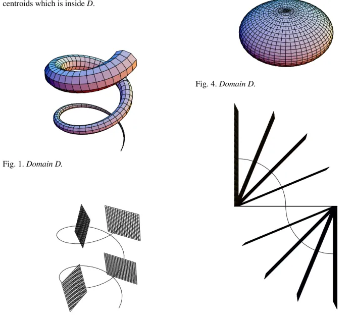
In the first example the curve c(t) is a curve of centroids which is insideD.
Fig. 1.Domain D.
Fig. 2. Curve of centroids and portions of planes Pt
orthogonal to the curve.
Fig. 3. Domain with some plane sections which give Dt.
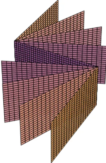
In the second example the curvec(t)is outside D and the scheme is similar to that of Cavalieri.
Fig. 4.Domain D.
Fig. 6.Planes Pt from another viewpoint.
Fig. 7.Domain with some plane sections and the curve c(t).
DISCUSSION
Stereological estimators of volume using a systematic scheme, based on equidistant cuts through a line, are usually much more precise than those based on independent sampling; because any systematic sample represents the whole material better than most samples obtained by independent sampling. Our estimator Eq. 20 preserves the systematic sampling scheme and offers the possibility to choose an alternative curve to a line whose orthogonal sample planes represent better the whole material.
On the other hand, our approach may be adapted to several clinical areas; for example, in the vessel study from IVUS (Intravascular Ultrasound) images, an artery can be modelled as a tube of non-constant
section (Fig. 3 is a particular case of these tubes), where the catheter trajectory is the curvec.
When the measurement function f(t)given in Eq. 19 is not known, its estimation will depend on the information provided in each practical case.
VOLUME OF DOMAINS
IN A SPACE FORM
Now we will extend Eq. 16 for compact domainsD in a simply connected space formMn
λ of dimensionn and sectional curvatureλ, withλ 6=0 (for λ =0 we have the results in Section 2). Let c:I = [0,L]−→ Mn
λ be a C∞ curve parametrized by its arc-length t and, for every t ∈ [0,L], let Pt denote a complete totally geodesic hypersurface of Mn
λ throughc(t) and orthogonal to the curvec. We suppose that there exists a Frenet frame alongc with the same properties as in Eq. 15 but f0
i(t) means, now, the covariant derivative of fi(t)alongc(t),
³∇ dtfi(t)
´ .
Under the same assumptions as in Eq. 1, each point xt ∈Dwill be given by
xt=expc(t)rtN(t) =expc(t)µ(t), (25)
where
µ(t) = n
∑
i=2µi
(t)Fi(t). (26)
Supposing now thatD⊂U, whereU is the image by exp of an open set of the normal bundle of c on which exp is a diffeomorphism, we may consider onU the coordinates:
φ(expc(t)rtN(t)) = (t,µ2(t), . . . ,µn(t)), (27) then
Voln(D) =
Z L
0
Z
Dth
∂t,τrf2(t)∧ ··· ∧τrfn(t)iσtdt, (28) where τr is the parallel transport from c(t) to
γN(t)(rt)(γN(t)is the geodesic withγN(t)(0) =c(t)and
γ0
N(t)(0) =N(t)). Now,
∂t= d
dt(expc(t)rtN(t)) =Y1(rt), (29) whereY1is the Jacobi field alongγN(t)satisfying:
which is given by Gray and Miquel (2000)
Y1(rt) =cλ(rt)τrf1(t) +sλ(rt)τrdt∇N(t), (31)
where, for every λ ∈R, sλ :R→R will denote the solution of the equation s00+λs=0 with the initial conditionss(0) =0 ands0(0) =1; andc
λ =s0λ; i. e.
sλ(s) =
sin(s√λ)/√λ, λ >0
s, λ =0
sinh(s√λ)/√λ, λ <0.
(32)
(Note that forλ=0,Y1(rt)is given by Eq. 7).
Finally, from Eq. 28 and Eq. 31 we have that
Voln(D) =
Z L
0 µZ
Dt
cλ(r)σt 
dt
+ Z L
0
Z
Dt sλ(rt)
¿∇
dtN(t),f1(t)
À
σtdt
= Z L
0
µZ
Dtcλ
(r)σt 
dt− Z L
0 MΓ2(Dt)k1(t)dt, (33)
where
MΓ2(Dt) =
Z
Dt
sλ(rt)hf2(t),N(t)iσt , (34)
and Eq. 33 generalizes Eq. 16 for space formsMn λ.
In the particular case where the compact domain D is obtained by a motion of a domain D0 through
the curvec(t); Eq. 33 has been obtained in Gray and Miquel (2000).
ABOUT THE CAVALIERI PRINCIPLE INMλn
The Cavalieri principle, already familiar to the ancient Greeks, states that the volumes of two solids in Rn are equal if the areas of the corresponding sections drawn perpendicular to a straight line are equal. This principle is not valid when totally geodesic hypersurfaces perpendicular to a given geodesic are considered; however, from Eq. 33 it is possible to formulate this principle for compact domains in Mn λ as follows:
Volumes of two compact domains in Mn
λ are equal
if the integrals Z
Dt
cλ(r)σt (35)
are equal through a geodesic c(t) in Mn
λ where r
denotes the geodesic distance from x to c(t).
(The integral Eq. 35 is equal to Voln−1(Dt) for
λ =0 and it is called the ‘modified volume’ in Choe and Gulliver (1992).)
ACKNOWLEDGEMENTS
The research was supported by the grant BSA2001-0803-C02-02. The author wishes to thank to the referees for helpful suggestions.
REFERENCES
Cruz-Orive LM, Roberts N (1993). Unbiased volume estimation with coaxial sections: an application to the human bladder. J Microsc 170:25-33.
Choe J, Gulliver R (1992). Isoperimetric inequalities on minimal submanifolds of space forms. Manuscripta Math 77:169-89.
Gray A, Miquel V (2000). Pappus type theorems on the volume in space forms. Ann Glob Anal Geom 18:241-54.
Gual-Arnau X, Cruz-Orive LM (1998). Variance prediction under systematic sampling with geometric probes. Adv Appl Probab (SGSA) 30:889-903.
Pache J C, Roberts N, Vock P, Zimmermann A, Cruz-Orive LM (1993). Vertical LM sectioning and parallel CT scanning designs for stereology: application to human lung. J Microsc 170:9-24.
Roberts N, Garden AS, Cruz-Orive LM, Whitehouse GH, Edwards RHT (1994). Estimating of fetal volume by magnetic resonance imaging and stereology. Brit J Radiol. 67:1067-77.
Treece G, Prager R, Gee A, Berman L (1999). Fast surface and volume estimation from non-parallel cross-sections, for freehand three-dimensional ultrasound. Med Image Anal 3:141-73.