(

(1)

INTERNATIONAL JOURNAL OF RESEARCH IN ELECTRONICS AND COMPUTER ENGINEERING A UNIT OF I2OR 2440 | P a g e

Impact of Bandwidth on LANDSAT-7 ETM+

Image Quality using Gaussian Filter: Mysore, INDIA

Choodarathnakara A L

1

_{, Bhagyamma S}

2

_{, Sandya M J}

3

_{, Sushmitha G R}

4

_{, Sowkya H K}

5

_{, Ramith H G}

6

Sinchana G S

7

_{, Satisha M}

8

_{and Ranjith Kumar K}

9 1,2,3,4,5,6,7,8,9

Government Engineering College, Kushalnagar-571234, Karnataka, INDIA

(E-mail:

[email protected], [email protected],[email protected]

)

Abstract— Gaussian filter smoothens digital images during

preserving edges, by re-evaluating every pixel. In computing the new pixel value, a window is centered on the pixel of interest with local neighborhood pixels. In this paper, Gaussian filtering technique implemented over LANDSAT-7 ETM+ satellite data product to analyze the impact of bandwidth. The recommendation of window is based on the statistical analysis which best enhances the image while preserving the edges. For satellite image with spatial resolution around 30m, window 3x3 for SD = 3, 3x3 for SD = 1.5, 9x9 for SD = 0.75 and 9x9 for SD = 0.375 are recommended. Resulting in blurred image, the largest window 9x9 was recommended to obtain better results.

Keywords— Gaussian Filter, Enhanced Edges, LANDSAT-7 ETM+

I. INTRODUCTION

In the image processing and computer vision Gaussian filter is extensively used. Signals get distorted when the noise is smoothed out. Gaussian filter is used for edge detection which also gives rise to edge position displacement, vanishing of edges and phantom edges. Authors have explained various techniques for noise removal problems. Gaussian filtering algorithm is later proposed, in which the filter variance is adapted for both noise characteristics and local variance of the signal [1]. In the theory of edge detection analysis proceeds in two parts, First, Changes which occur in a natural image over a wide range of scales are identified distinctly at different scales and intensity changes in images arise from surface discontinuities [2].

In the image, edge detection is the task of determining and focusing changes of light intensity. As discussed by V. Terre and T. Poggio (1984), edge detection is a problem of numerical differentiation. Author shows the regularization techniques, which leads to filtering the image earlier to the suitable differentiation operation. This process is equivalent to convolving the data with the desired derivative of a generalized spline filter [3]. The optimal detector has a simple approximate implementation in which edges are marked at maxima in gradient magnitude of a Gaussian-smoothed image. Author prolonged this finder using operators of several widths to cope with different signal-to-noise ratios in the image. The impulse response of the optimal step edge operator was shown to approximate the first derivative of a Gaussian [4].

Andres Huertas and Gerard Medioni have proposed technique that takes a gray level image as input, locates edges with sub pixel accuracy, and links them into lines. Edges are detected by finding zero-crossings in the convolution of the image with Laplacian-of-Gaussian (LoG) masks. Authors locate zero- crossings with pixel precision that is the edge on the pixel which has the smallest absolute value [5]. Fast calculation of edge and ridge maps were done by anisotropic Gaussian filtering method with high spatial and angular accuracy. Convolution filtering is advantageous when considering locally steered filtering. But, as is the case of tracking applications recursive filtering is more attractive when smoothing or differentiating the whole image array [6].

The various features of Gaussian operator that make it the filter of choice in the area of edge detection are discussed. Despite these desirable features of the Gaussian filter, edge detection algorithms with associated problems are highlighted [7]. Scale-space filter constructs the hierarchic symbolic signal descriptions by converting the signal into a continuum of versions of the original signal convolved with a kernel containing a scale or bandwidth parameter. It is shown that the Gaussian probability density function is the only kernel in a broad class for which first-order maxima and minima respectively, increase and decrease when the bandwidth of the filter is increased [8].

II. STUDY AREA AND DATA PRODUCTS Mysore is the cleanest city in the Karnataka; India located about

146 km from the state capital. It has an average altitude of 770 meters and spread across an area of 128.42 km2_{. During}

2001, the land area used in Mysore city was 16.1% roads, 39.9% residential, 13.48% industrial, 13.74% parks and open spaces, 3.02% commercial, 2.02% water, 8.96% public property and 2.27% agriculture.

The description of satellite image used in this testing is depicted in Table 1. The data are of LANDSAT-7 ETM+ obtained from United States Geological Survey (USGS) and Google Earth. The Table 2 shows LANDSAT-7 ETM+ data bands along with ground features.

(2)

INTERNATIONAL JOURNAL OF RESEARCH IN ELECTRONICS AND COMPUTER ENGINEERING A UNIT OF I2OR 2441 | P a g e Fig 1: Google Earth Snapshot of Mysore Rural and

Urban Study Area

Table 1: Specifications of Satellite Data Products used

Table 2: LANDSAT-7 ETM+ Bands along with Ground Features

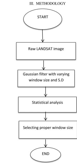
III. METHODOLOGY

Fig 2: Proposed Methodology for Image Quality using Gaussian Filter

The methodology adapted as shown in Fig 2 to assess the impact of bandwidth on satellite image using Gaussian filter. During the

first phase of the experiment, the data was procured and pre-processed. Gaussian filter was applied with varying window

sizes 3x3, 5x5, 7x7, 9x9 for standard deviations 3, 1.5, 0.75, 0.375 respectively. Finally, proper window size was selected based on statistical analysis viz Mean, SD and SNR.

S L . N o

Satellite and Data Type

Date of Acquisi tion

Spectral Resolution Spatial

Resoluti on

1 .

Land Sat ETM 7

2010 Blue (0.45-0.515m) Green (0.525- 0.605m)

Red (0.632-0.69m) Near Infrared (0.75- 0.90m)

Short wave IR-1 (1.55-1.75m) Thermal IR (10.4- 12.5m)

Short wave IR-2 (2.09-2.35m)

30.0m

2 .

Google Earth

April

2016

-

Ground Feature Bands Used

Water 1,2,3; 1,2,4; 1,4,5

Urban 1,2,3; 1,4,5

Farmland 1,2,3; 1,4,5

Forest 1,2,3; 1,4,5

Salt scald 1,2,3

Scrub 1,4,5

Vegetation 1,4,7

START

Raw LANDSAT image

Gaussian filter with varying window size and S.D

Statistical analysis

Selecting proper window size

(3)

INTERNATIONAL JOURNAL OF RESEARCH IN ELECTRONICS AND COMPUTER ENGINEERING A UNIT OF I2OR 2442 | P a g e IV. EXPERIMENTAL RESULTS

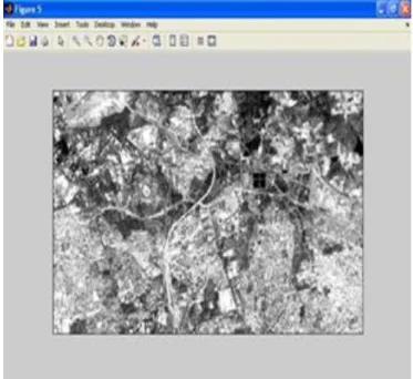
Fig 3 depicts the gray scale image of LANDSAT-7 ETM+ data considered during this experiment. Fig 4 shows the Gaussian filter response for 3x3 size window with standard deviation 0.375 producing mean value of 147.0181 and standard deviation of 57.4985.

Fig 3: Conversion of LANDSAT Image into Gray Scale

Fig 4: 3x3 Size Windows with Standard Deviation 0.375

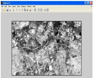
Fig 5 shows the Gaussian filter response for 3x3 window size with standard deviation 0.75 producing mean value of 147.0295 and standard deviation of 58.0898. Fig 6 shows the Gaussian filter response for 3x3 window size with standard deviation 1.5 producing mean value of 147.2009 and standard deviation of 59.0779.

Fig 5: 3x3 Size Window with Standard Deviation 0.75

(4)

INTERNATIONAL JOURNAL OF RESEARCH IN ELECTRONICS AND COMPUTER ENGINEERING A UNIT OF I2OR 2443 | P a g e Fig 7 shows the Gaussian filter response for 3x3 window size

with standard deviation 3 producing mean value of 147.6440 and standard deviation of 66.8350. Fig 8 shows the Gaussian filter response for 5x5 window size with standard deviation 0.375 producing mean value of 146.2735 and standard deviation of 53.5868.

Fig 7: 3x3 Size Window with Standard Deviation 3

Fig 10

Fig 10: 5x5 Size Window with Standard

Deviation 1.5

(5)

(6)

Fig 18: 9x9 Size Window with Standard Deviation 1.5.

(7)

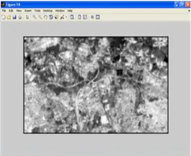
INTERNATIONAL JOURNAL OF RESEARCH IN ELECTRONICS AND COMPUTER ENGINEERING A UNIT OF I2OR 2446 | P a g e Fig 19: 9x9 Size Window with Standard Deviation 3

Fig 19 shows the Gaussian filter response for 9x9 window size with standard deviation 3 producing mean value of 143.9104 and standard deviation of 69.2592.

Table 3. Statistical Measures of Gaussian Filter for Different Size & SD

Filter Window Standard Deviation Filter Window

Size Min Max Mean

Standard

Deviation SNR

1 255 147.4123 67.5939 2.1755

3 3 x 3 0 255 147.6440 66.8350 2.2090

3 5 x 5 0 255 146.8167 68.4499 2.1448 3 7 x 7 0 255 146.2569 67.3275 1.5026 3 9 x 9 0 255 143.9104 69.2592 2.0778

1.5 3 x 3 0 255 147.2009 59.0779 2.916

1.5 5 x 5 0 255 145.9870 59.4885 2.4540 1.5 7 x 7 0 255 144.7349 60.8659 2.378 1.5 9 x 9 0 255 144.7788 60.5960 2.3892 0.75 3 x 3 0 255 147.0295 58.0898 2.5312 0.75 5 x 5 0 255 145.8676 55.1626 2.6443 0.75 7 x 7 0 255 144.7191 55.0351 2.6295

0.75 9 x 9 0 255 144.7086 54.7057 2.6454

0.375 3 x 3 0 255 147.0181 57.4985 2.5569 0.375 5 x 5 0 255 146.2735 53.5868 2.7296 0.375 7 x 7 0 255 145.2860 52.1160 2.7877

0.375 9 x 9 0 255 145.0560 50.7162 2.8600

Analyzing the statistical values depicted in Table 3, selection of better window can be made for various standard deviations viz. 3, 1.5, 0.75 and 0.375. From Table 3, for window with standard deviation of 3, the filter window size 3x3 was recommended to enhance the image quality while preserving the edges. Similarly, for window with standard deviation of 1.5, the filter window size 3x3 was recommended. For window with standard deviation of 0.75, the filter window size 9x9 was recommended. For window with standard deviation of 0.375, the filter window size 9x9 was recommended.

V. CONCLUSION

The recommendation of window is performed based on the statistics which best improves the quality of image while retaining the edges. The Gaussian filtering approach to preserve the image quality of satellite image with high resolution around 30 m, window size 3x3 for SD = 3, window size 3x3 for SD = 1.5, window size 9x9 for SD = 0.75 and window size 9x9 for SD = 0.375 are recommended. Resulting in blurred images, the largest window size 9x9 was recommended to obtain better results. The Gaussian filtering technique can be implemented further for different satellite data products of interest. The Gaussian filtering technique can be implemented further for more than 9x9 window sizes to analyze the impact of bandwidth as well.

ACKNOWLEDGMENT

Special thanks to Mr. Nasser Mustafa Saleh Abdin for encouragement, guidance and other contributions to this study. All the LANDSAT-7 ETM+ data used in this work is downloaded from the USGS web (http://glovis.usgs.gov), special thanks to the group. The authors would like to thank anonymous reviewers for their valuable comments. Also, the authors would like to graciously thank National Remote Sensing Centre (NRSC), Hyderabad, INDIA for providing the data product for the study. Thanks to the Survey of India (SOI) for providing the Topographic Maps for this study and Karnataka State Remote Sensing Application Centre (KSRSAC), Bangalore.

REFERENCES

[1] G. Deng and L. W. Cahill, 1994. “An Adaptive Gaussian Filter

for Noise Reduction and Edge Detection”, IEEE.

[2] D. Marr and E. Hildreth, 1980. “Theory of Edge Detection”

Proc. R. Soc. Lond. B 207, 187-217.

[3] T. Poggio, H. Voorhees, and A. Yuille, 1988. “A Regularized

Solution to Edge Detection” journal of complexity 4, 106-123.

[4] John Canny, 1986. "A Computational Approach to Edge

Detection", IEEE. Transactions on pattern analysis and machine intelligence, Vol.pami-8, No.6.

[5] Andres Huertas and Gerard Medioni, 1986. “Detection of

Intensity Changes with Subpixel Accuracy Using Laplacian- Gaussian Masks”, IEEE. Vol. PAMI-8, No.5.

[6] Jan-Mark Geusebroek, W. M. Arnold, Smeulders, Member,

IEEE., and Joost van de Weijer, 2003 “Fast Anisotropic Gauss Filtering” Vol. 12, No.8.

[7] Mitra Basu, Senior Member, 2002. “Gaussian-Based Edge-

Detection Methods—A Survey”, IEEE. Vol. 32, No. 3.

[8] Jean Babaud, P. Andrew, Witkin, Michel Baudin, Member,

IEEE, and Richardo, Duda, Fellow, 1986. “Uniqueness of the Gaussian Kernel for Scale-Space Filterng”. IEEE transactions on pattern analysis and machine intelligence. Vol. PAMI-8, No.5.

(8)

INTERNATIONAL JOURNAL OF RESEARCH IN ELECTRONICS AND COMPUTER ENGINEERING A UNIT OF I2OR 2447 | P a g e

. , . .

Ramith H G, USN: 4GL14EC043,

Department of Electronics &

Communication Engineering,

Government Engineering College, Kushanagar-571234, South Kodagu, Karnataka, INDIA affiliated to

Visvesvaraya Technological

University, Belagavi, INDIA. He was born in Hassan District of Karnataka State in INDIA.

Sowkya H K, USN: 4GL15EC047,

Government Engineering College, Kushanagar-571234, South Kodagu, Karnataka, INDIA affiliated to

Visvesvaraya Technological

University, Belagavi, INDIA. She was born in Tiptur taluk of Karnataka State in INDIA.

Ranjithkumar K, USN:

4GL16EC413, Department of

Electronics & Communication

Engineering, Government

Engineering College, Kushanagar-571234, South Kodagu, Karnataka, INDIA affiliated to Visvesvaraya Technological University, Belagavi, INDIA. He was born in Bangalore Rural District of Karnataka State in INDIA.

Satish M, USN: 4GL15EC036,

Government Engineering College,

Kushanagar-571234, South

Kodagu, Karnataka, INDIA

affiliated to Visvesvaraya

Technological University, Belagavi,

INDIA. He was born in

Chikballapur District of Karnataka State in INDIA.

Sinchana G S, USN:

4GL15EC045, Department of

Engineering College, Kushanagar-571234, South Kodagu, Karnataka, INDIA affiliated to Visvesvaraya

Technological University,

Belagavi, INDIA. She was born in Mandya District of Karnataka State in INDIA.

Bhagyamma S was born in Mandya District of Karnataka State in INDIA. She received B.E.

degree in Electronics &

Communication Engineering in the year 2000, M.Tech. degree in Industrial Electronics in the year 2008 from NIE, Mysore and SJCE, Mysore respectively.

Choodarathnakara A L was born in Hassan District of Karnataka State in INDIA. He received B.E. degree in Electronics & Communication Engineering in the year 2002,

M.Tech. degree in Digital

Systems in the year 2008 and Ph.D

from Malnad College of

Engineering, Research Centre,

Hassan affiliated to Visvesvaraya Technological University, Belagavi, INDIA.

Sandya M J, USN:

4GL15EC033, Department of Electronics & Communication

Engineering College,

Belagavi, INDIA. She was born in Hassan District of Karnataka State in INDIA.

presently, he is working as an Associate Professor in the Department of Electronics & Communication Engineering, Government Engineering College, Kushalnagar-571234, Kodagu District, Karnataka State, INDIA. He is a Life Member of the Indian Society of Technical Education (ISTE-43168), Indian

Society of Remote Sensing (ISRS-3533), Indian Society of

Geomatics (ISG-1258), Member of International Association of Engineers (IAENG-143588), Member of the IAENG Society of Artificial Intelligence, Member of the IAENG Society of Data Mining and Member of the IAENG Society of Imaging Engineering.

E-mail: [email protected]

Presently, she is working as an Assistant Professor in the Department of Electronics & Communication Engineering, Government Engineering College, kushalnagar-571234, Kodagu District, Karnataka State, INDIA.

E-mail: [email protected]

Sushmitha G R, USN:

4GL15EC043, Department of Electronics & Communication

Engineering College,

Belagavi, INDIA. She was born in Mandya District of Karnataka State in INDIA.