Experimental Computer Science:
The Need for a Cultural Change
Dror G. Feitelson
School of Computer Science and Engineering The Hebrew University of Jerusalem
91904 Jerusalem, Israel
Version of December 3, 2006
Abstract
The culture of computer science emphasizes novelty and self-containment, leading to a fragmentation where each research project strives to create its own unique world. This ap-proach is quite distinct from experimentation as it is known in other sciences — i.e. based on observations, hypothesis testing, and reproducibility — that is based on a presupposed common world. But there are many cases in which such experimental procedures can lead to interesting research results even in computer science. It is therefore proposed that greater acceptance of such activities would be beneficial and should be fostered.
1
Introduction
“Research is the act of going up alleys to see if they are blind.”
Plutarch
“In all affairs it’s a healthy thing now and then to hang a question mark on the things you have long taken for granted.”
Bertrand Russell
We know what theoretical computer science is: the study of what can be computed and at what cost. But what is experimental computer science? Looking to other branches of science for inspiration, we can find three components that define experimental science:
1. Observation 2. Hypothesis testing 3. Reproducibility
The question is how and whether these apply to computer science. We will attempt to answer this in the sequel.
As the nature of computer science and the possible role of experimentation have already been debated at length by others, we first review these discussions in the remainder of this section. While this provides many historical insights, it is also possible to skip directly to our main arguments which start in Section 2.
1.1
Computer Science
“A science is any discipline in which the fool of this generation can go beyond the point reached by the genius of the last generation.”
Max Gluckman
Computer science is a young and constantly evolving discipline. It is therefore viewed in different ways by different people, leading to different perceptions of whether it is a “science” at all [13]. These discussions periodically beget reports on the subject, such as the “Computing as a discipline” report by Denning at al. [16].
Of course, it all boils down to definitions. One interesting distinction considers three possible classifications:
Science — this is concerned with uncovering the laws of the universe. It is an analytic activity, based on observing the real world. Obvious examples are physics, chemistry, and biology. Engineering — this is concerned with building new things that are practically useful. Thus it
is a synthetic activity. Examples include mechanical engineering, civil engineering, and electrical engineering.
Mathematics — this is concerned with the abstract, and may be considered to verge on the philo-sophical. It includes the construction and study of abstract processes and structures, such as in set theory, graph theory, and logic. While these are obviously used in both science and engineering, their development is often independent of any such potential use.
Research in computer science is typically part of the latter two classifications. Much of computer science is about how to do things that have not been done before, or in other words, inventing new algorithms [29] and building new tools [5]. This spans a very wide spectrum of activities, from information retrieval to animation and image processing to process control. While in many cases this does not have the feel of hard-core engineering, it is nevertheless an activity that leads to the creation of new tools and possibilities.
By contradistinction, the non-algorithmic parts of theoretical computer science (such as plexity theory) are more philosophical in nature. Their domain of study is inspired by real com-puters, but it is then abstracted away in the form of models that can be studied mathematically. Structures such as the polynomial hierarchy are the result of a thought process, and do not cor-respond to any real computational devices. This is proper, as this theory deals with information, which is not subject to physical laws [29].
But computer science seems to have relatively few examples in the first category, that of ob-serving, describing, and understanding something that was just there. Our contention is that the techniques used for these activities in the natural sciences have good uses in computer science as well, and that there are in fact things to be found. As a motivating example, consider the finding of self-similarity in computer network traffic. Up to the early 1990s, the prevailing (abstract) model of traffic was that it constituted a Poisson process. But collecting real data revealed that this was not the case, and alternative fractal models should be employed [38]. This was an observation of how the world behaves, that was motivated by scientific curiosity, and led to an unexpected result of significant consequences.
1.2
Experimentation
“when we ignore experimentation and avoid contact with the reality, we hamper progress.”
Walter Tichy
“The only man I know who behaves sensibly is my tailor; he takes my measurements anew each time he sees me. The rest go on with their old measurements and expect me to fit them.”
George Bernard Shaw
“Beware of bugs in the above code; I have only proved it correct, not tried it.”
Donald Knuth
An immediate objection to the above comments is that experimental computer science is actu-ally widely practiced. In fact, three distinct definitions of what constitutes experimental computer science can be identified.
Perhaps the most prominent use of the term “experimental computer science” occurs in several NSF reports, e.g. the Rejuvenating experimental computer science report from 1979 [23], and the Academic careers for experimental computer scientists and engineers report from 1994 [46]. However, these reports don’t really attempt to define experimental science; rather, they use the phrase “experimental computer science” as a counterpart to “theoretical computer science”. As such, this is an umbrella term that covers university research that includes the building of real systems, and therefore needs to be treated differently in terms of funding and expected generation of papers. The justification for such special treatment is the expectation of a relatively direct effect on technological progress.
The core of this notion of experimental computer science is the building of systems, whether hardware or software. This is not done so much to study these systems, as to demonstrate their fea-sibility [29]. Thus it is more of an engineering activity than a scientific one. And indeed, one of the reports notes that this notion of experimental computer science is largely divorced from the theory of computer science, as opposed to the relatively tight coupling of theory and experimentation in the natural sciences [46].
The second notion of experimental computer science is that used by Denning in his paper
hypothesis or model observation
test experimental
idea
system design evaluation
experimental
implementation predictionconcrete concrete
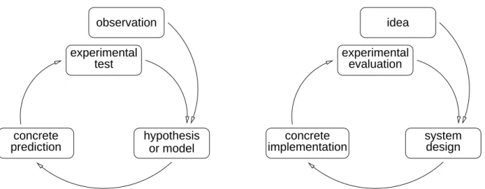
Figure 1: A comparison of the scientific method (on the left) with the role of experimentation in system design (right).
that the essence of experimental science is the modeling of nature by mathematical laws; therefore, experimental computer science is the mathematical modeling of the behavior of computer systems. Moreover, it is suggested that studying the abstract models qualifies as experimentation. This no-tion is carried over to the report Computing as a discipline [16], where modeling and abstracno-tion are proposed as one of the three basic paradigms that cut across all of computer science (the other two being theory and design).
But Denning also mentions the use of experimentation as a feedback step in the engineering loop: a system is designed that has anticipated properties, but these are then tested experimentally. If the results do not match the expectations, the system design is modified accordingly (Fig. 1). One of Denning’s examples of such a cycle is the development of paging systems that implement virtual memory, which didn’t provide the expected benefits until the page replacement algorithms were sufficiently refined [15]. This was achieved by a combination of abstract modeling and ex-perimental verification.
In fact, using experimental feedback can be argued to be the dominant force underlying the progress of the whole of computer science. This claim is made by Newell and Simon in their Turing Award lecture [47]. They start by noting that “the phenomena surrounding computers are deep and obscure, requiring much experimentation to assess their nature”. While they admit that the nature of this experimentation “do[es] not fit a narrow stereotype of the experimental method”, they claim that it is nevertheless an experimental process that shapes the evolution of new ideas: you can’t really decide if a new idea is good until you try it out. As many ideas are tried by many people, the good ones survive and the bad ones are discarded. This can even lead to the formation of fundamental hypotheses that unite the work in a whole field. As an example, they cite two such hypotheses that underlie work in artificial intelligence: one that a physical symbol system has the necessary and sufficient means for general intelligent action, and the other that intelligent behavior is achieved by heuristic search.
mod-est and concrete scale. It involves the evaluation of computer systems, but using (more of) the standard methodologies of the natural sciences. This approach is advocated by Tichy in his paper
Should computer scientists experiment more? [62], and by Fenton et al. in the paper Science and substance: a challenge to software engineers [24]
A possible argument against such proposals is that experimentation is already being done. Many systems-oriented papers include “experimental results” sections, which present the results obtained through simulations or even measurements of real implementations [13]. In addition, there are at least two journals and a handful of workshops and conferences devoted to empirical studies:
• The ACM Journal of Experimental Algorithmics, which is devoted to empirical studies of algorithms and data structures. Its mere existence reflects the understanding that such studies are needed, because some algorithms may simply be too complex to analyze. Experimenta-tion may also be needed to augment worst-case behavior with an assessment of the typical case.
• The Springer journal Empirical Software Engineering. Here the use of experimentation is a result of the “soft” nature of the material: software construction is a human activity, and cannot be modeled and analyzed mathematically from first principles [24].
• The annual Text REtrieval Conference (TREC) is a forum created by NIST specifically to promote and standardize the experimental evaluation of systems for information retrieval [66]. In each year, a large (averaging 800,000) corpus of documents is created, and a set of 50 query topics is announced. Participants then use their respective systems to find topic-related documents from the corpus, and submit the results for judging.
• The annual Internet Measurement Conference (ICM), which includes papers that study the Internet as a complex structure that — despite being man-made — needs to be studied ex-perimentally, often relying on deductions based on external measurements.
• The Workshop on Duplicating, Deconstructing, and Debunking (WDDD), held annually with ACM’s International Symposium on Computer Architecture (ISCA), which includes this wording in its call for papers:
Traditionally, computer systems conferences and workshops focus almost exclu-sively on novelty and performance, neglecting an abundance of interesting work that lacks one or both of these attributes. A significant part of research—in fact, the backbone of the scientific method—involves independent validation of exist-ing work and the exploration of strange ideas that never pan out. This workshop provides a venue for disseminating such work in our community.
• The International Symposium on Empirical Software Engineering (ISESE), which is ex-pected to merge with the International Symposium on Software Metrics to form a conference devoted to Empirical Software Engineering and Measurement in 2007.
• The International Symposium on Experimental Robotics, a bi-annual meeting focusing on theories and principles which have been validated by experiments.
While this listing is encouraging, it is also disheartening that most of these venues are vary narrow in scope. Furthermore, their existence actually accentuates the low esteem by which experimental work is regarded in computer science. For example, the Internet Measurement conference web site states
IMC was begun as a workshop in 2001 in response to the difficulty at that time find-ing appropriate publication/presentation venues for high-quality Internet measurement research in general, and frustration with the annual ACM SIGCOMM conference’s treatment of measurement submissions in particular.
Despite the existence of several experimentally oriented venues, this fraction of papers and journals is much lower than in other scientific fields [63]. Moreover, in many cases system ex-periments are more demonstrations that the idea or system works than a real experiment (what constitutes a “real” experiment is detailed below, e.g. in Section 2.3). In the following sections, we hope to show that there is much more than this to experimental methodology.
Another problem with the experimental approach used in many papers is that the methodology is inadequate. Fenton et al. write [24]
Five questions should be (but rarely are) asked about any claim arising from software-engineering research:
• Is it based on empirical evaluation and data?
• Was the experiment designed correctly?
• Is it based on a toy or a real situation?
• Were the measurements used appropriate for the goals of the experiment?
• Was the experiment run for a long enough time?
In addition, comparisons with other work may be inadequate due to lack of real experience and understanding of the competing approaches [68]. In the systems area, a common problem is the lack of objectivity. Inevitably, experimental and comparative studies are designed and executed by an interested party. They don’t measure an independent, “real” world, but rather a system they had created at substantial investment, and opposite it, some competing systems. In particular, there is practically no independent replication of the experiments of others. Thus reported experiments are susceptible to two problems: a bias in favor of your own system, and a tendency to compare against restricted, less optimized versions of the competition [6, 70]. Obviously, both of these might limit the validity of the comparison.
The goal of the present paper is not to argue with the above ideas; in fact, we totally accept them. However, we claim that there is more to experimental computer science. In the following sections, we return to the three basic components of experimental science and try to show that
• There is a place for observation of the real world, as in the natural sciences,
• There is a use for hypothesis testing at an immediate and direct level as part of the evaluation and understanding of man-made systems, and
• There is a need for reproducibility and repetition of results as advocated by the scientific method.
And while this may be done already to some degree, it would be beneficial to the field as a whole if it were done much much more.
2
Observation
“Discovery consists in seeing what everyone else has seen and thinking what no one else has thought.”
Albert Szent-Gyorgi
In the exact sciences observation means the study of nature. In computer science this means the measurement of real systems. Note that we exclude simulation from this context. This is analogous to the distinction between experimental and computational approaches to other sciences.
Measurement and observation are the basis for forming a model of the world, which is the essence of learning something about it. The model can then be used to make predictions, which can then be tested — as discussed in Section 3.
It should be noted that model building is not the only reason for measurement. Another goal is just to know more about the world in which we live and operate. For example, what is the locking overhead or scheduling overhead of an operating system? What is the distribution of runtimes of processes? What is the behavior of systems that fail? Knowing the answers to such questions can serve to shape our world view and focus the questions we ask.
Making measurements for the sake of measurements is uncommon in computer science. The culture favors self-containment and the presentation of a full story, rather than “just” measure-ments. Our views on why “just measurements” should be tolerated and even encouraged are elab-orated in the subsections below.
2.1
Challenges
“Art and science have their meeting point in method.”
Edward Bulwer-Lytton
“Genius is the talent for seeing things straight.”
Maude Adams
The prevailing attitude of many computer scientists seems to be that measurements are just done. In reality, it is indeed very easy to obtain unreliable measurements. But making reliable measurements can be quite challenging [51]. Regrettably, it may also be quite difficult to distin-guish between the two.
Consider the question of determining the overhead of a context switch, for example. On the face of it it seems like a rather simple thing to do. In fact, it can even be done by a user-level process. For example, Ousterhout proposed to measure context switches by creating two processes
that continually send each other a single byte via a pipe [48]. The operating system will then continually switch between them, because each process blocks trying to read the other process’s byte immediately after sending its own byte. Thus measuring the time to pass a byte a thousand times is essentially a measurement of a thousand context switches.
However, such measurements can only provide an approximation of the context switch’s over-head. Some of the problems are
1. We are also measuring the time to read and write bytes to a pipe. To factor this out, we need to measure these activities separately and subtract them from the context switch overhead. 2. It might happen that some system daemon or other process wakes up and is scheduled
be-tween our two processes. In this case we are measuring two context switches and whatever this other process does too.
3. The resolution of the system timer might be insufficient to measure a single context switch. Even if time is given in microseconds, it does not mean that the resolution is single mi-croseconds — an implementation may actually only support millisecond resolution, and always return time values that are integral multiples of 1000 microseconds. Therefore re-peated context switches need to be performed to make the total overhead measurable. This increases the danger of interference as noted above from system daemons, and in addition the loop overhead should also be accounted for. An alternative is to use a cycle counter, as is provided on most modern architectures. However, accessing a cycle counter actually takes more than a cycle, and care must be taken to handle wrap-around.
A promising alternative that at least ensures we know exactly what we are measuring is to make the measurement within the operating system’s kernel. We can identify the kernel code responsible for context switching, and simply time it. But this is actually not as easy as it sounds [17]. It requires intimate knowledge of the system, e.g. in case the code has more than one exit point.
Another problem is that the phrase “context switch overhead” is actually not well-defined. It could mean at least three different things:
1. The time that the operating system runs in order to perform a context switch.
2. The time from when one user process stops running till when the next user process starts running. This is slightly longer than the time the operating system runs, as it includes the trap into the operating system and the return to user level.
3. The “lost” time that user processes cannot use due to the context switch. This may be much longer than the direct overhead indicated above, as there may be additional lost time due to lost cache state that needs to be restored. Note that this has two sub-cases: cache lines that were lost due to the operating system activity, and cache lines lost due to the activity of other processes since the last time this process ran.
In addition, these values are not singular, but rather come from a distribution: if you repeat the measurement many times, you will get different numbers, and the variability may be significant.
Of course, these problems are not unique to trying to measure the context switch overhead. Once you start thinking about it, similar problems pop up regarding practically any measurement. For example, how would you measure memory bandwidth, and what does it means when you have multiple levels of caching? How do you measure processor throughput when you have superscalar out-of-order execution and multiple functional units?
It should also be stressed that all the above relates to the simplest and most basic of measure-ments. This goes to show that various decisions have to be made in the process of measurement, some of which may have subtle implications. It is reasonable that different people will have dif-ferent opinions about what decisions to make. Such differences can only be resolved (or acknowl-edged) by a social process of discussing the alternatives and seeing which are found to be most useful in practice.
In addition, it is necessary to develop measurement methodologies that avoid perturbations of the measured system, and are applicable to different situations. For example, one can use a large memory-mapped buffer to accumulate measurements, and flush it to disk only at the end of the measurement period. This reduces perturbations during the measurement (provided the buffer does not overflow), at the price of reducing the memory available to the measured system, which in principle may also cause a change in behavior. Which effect is more troublesome can only be determined by experience. Such methodologies and experience need to be shared by researchers, in order to avoid duplication of effort and achieve uniformity of standards. This can only be done effectively in a culture that appreciates the intellectual effort and expertise needed to perform reliable measurements.
2.2
Metrics
“When you can measure what you are speaking about and express it in numbers, you know something about it.”
Lord Kelvin
“If you can’t measure it, you can’t improve it.”
unknown
A special challenge in performing measurements is coming up with appropriate metrics. In physics, there are a few basic units that can be measured: length, time, mass, charge, etc. Then there are a few derived units: speed is length divided by time, current is charge divided by time, and so on. Part of the substance of physics is to find relationships between units, e.g. different combinations that all yield variants of energy.
But what are the units of computer science measurements? One obvious candidate, shared with physics, is time: we are practically obsessed with how long things take, and even more, with throughput, i.e. how many things we can do per unit of time (MIPS, MFLOPS, MB/s, etc.). But there are many notions that are hard to measure because we don’t have good metrics.
Maybe the most prominent example is locality. Locality of reference is a very basic notion in computer science, and underlies the myriad versions of caching, including processor caches, file system buffer caches, and web proxy caches. We all know about the distinction between spatial
SDSC HTTP
0 100 200 300 400 500 600
stack distance
0 300 600 900 1200 1500
number of references
0
SDSC HTTP
stack distance
0 300 600 900 1200 1500 1800
survival probability
1 0.1 0.01 0.001 0.0001 0.00001
original trace scrambled trace
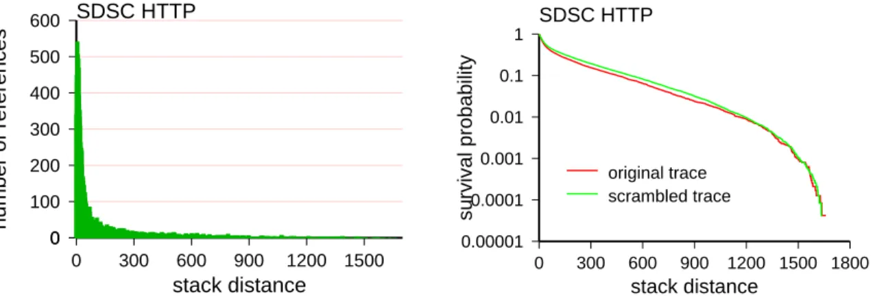
Figure 2: Left: histogram of stack distances for a log of HTTP requests from a SDSC web server. Right: difference in the tail of the stack-distance distributions for the original data and scrambled data.
locality and temporal locality. But how does one measure locality? Given a computer program, can you find a number that represents the degree of locality that it exhibits? Can you compare two programs and say with confidence which has more locality? Does any course in the computer science curriculum discuss these issues?
The truth of the matter is that there has been some work on measuring locality. The most popular metric is the average stack distance [60]. Given a reference stream, insert each new address into a stack. If the address is already in the stack, note its depth and move it to the top. The average depth at which addresses are found is the desired metric: if the program exhibits strong locality, items will be found near the top of the stack, and the average stack distance will be small. If there is no locality, the average stack distance will be large.
The average stack distance is a simple metric with intuitive appeal. However, it is seldom actually used. There are two reasons for this situation. First, it only measures temporal locality, and there is no corresponding simple metric for spatial locality. Second, temporal locality is actually the combination of two separate effects:
1. A correlation between an item and nearby items in the reference stream, which tend to be the same, and
2. A skewed popularity, where some items are much more common than others, and therefore appear much more often in the reference stream.
The intuition of locality leans towards the first effect: we think of locality in terms of references to the same item that are bunched together at a certain time, and are absent at other times. But in reality, the second effect may be much stronger.
An example is shown in Fig. 2. The left-hand graph is a histogram of the stack distances ob-served in a well-known data log, the SDSC HTTP trace available from the Internet Traffic Archive. This trace contains 25,430 successful requests to 1680 unique files, which were logged on August
22, 1995. The distribution shows remarkable locality, as low values are extremely common. How-ever, the distribution hardly changes when the log is scrambled, and the same requests are viewed in an arbitrary random order. This implies that the low stack distances are the result of a few items being very popular, and not of a correlation structure in the reference stream. And indeed, it is well-known that popularity often follows the highly skewed Zipf distribution [4].
The bottom line is then that we don’t know of a simple metric for locality, and in particular, for separating the different types of locality. This is actually a pretty common situation. We also don’t really know how to measure the quantity, quality, or complexity of software, or the productivity of software production, the performance of microprocessors or supercomputers, or the reliability or availability of distributed systems, to mention but a few. It’s not that no metric is available. It’s that the suggested metrics all have obvious deficiencies, none are widely used, and that there is relatively little discussion about how to improve them.
Of course, coming up with good metrics is not easy. One should especially beware of the temptation of measuring what is easily accessible, and using it as a proxy for what is really required [51]. Baseball statistics provide an illuminating example in this respect [39]. Players were (and still are) often evaluated by their batting average and how fast they can run, and pitchers by how fast they can throw the ball. But as it turns out, these metrics don’t correlate with having a positive effect on winning baseball games. Therefore other metrics are needed. What metrics are the most effective is determined by experimentation: when you have a candidate metric, try it out and see if it makes the right predictions. After years of checking vast amounts of data by many people, simple and effective metrics can be distilled. In the case of baseball, the metric for hitters is their on-base percentage; for pitchers it is hitters struck out and home runs allowed.
Many additional examples of measuring things that initially may seem unmeasurable can be found in the fields of cognitive psychology and behavioral economics. Especially famous is the work of Kahneman and Tversky, regarding the biases effecting economic decision making. For example, they designed experiments that showed that people tend to give potential losses twice as much weight as that assigned to potential gains. Such data helped explain what was seen as irrational economic behavior, and eventually led to the awarding of the 2002 Nobel Prize in eco-nomics.
2.3
Surprises
“I didn’t think; I experimented.”
Wilhelm Roentgen
“The most exciting phrase to hear in science, the one that heralds the most discoveries, is not “Eureka!”, but “That’s funny...””
Isaac Asimov
“There are two possible outcomes: if the result confirms the hypothesis, then you’ve made a measurement. If the result is contrary to the hypothesis, then you’ve made a discovery.”
“Fiction is obliged to stick to possibilities. Truth isn’t.”
Mark Twain
An essential element of experimental measurements is the potential for surprises. This is what distinguishes true experimental exploration from demonstrations and calibrations of system mod-els. Experiments are out to obtain new (and unexpected) knowledge. In fact, this is what science is all about, as articulated in John Henry’s writing about the genesis of the scientific method at the hands of Francis Bacon [32]:
Before Bacon’s time, the study of nature was based largely on armchair speculation. It relied almost entirely on abstract reasoning, starting from a restricted range of presup-positions about the nature of the world, and its aim was to explain known phenomena in ways that were consistent with those presuppositions. We now know that these presuppositions were incorrect and that much of pre-modern natural philosophy was therefore entirely misconceived, but this would never, could never, have been realised by anyone working within the tradition...
Without experiments, nature doesn’t have the opportunity to tell you anything new. The same goes for computer-based systems.
Perhaps the best-known example of a surprising discovery (in the context of computer sys-tems) emanating from empirical measurements is the discovery of self-similarity in network traffic [38]. This started with the seemingly pointless collection of voluminous data regarding packets transmitted on an Ethernet local area network — an observation of the real world. Analyzing this data showed that it does not conform with the prevailing Poisson models of traffic. In particular, aggregating the data over increasing time scales did not lead to a fast reduction in variance as was expected. This led to the creation of the self-similar network traffic models that are now accepted as much more realistic. And this is not only of academic interest: the new models have major implications regarding the design of communication systems, e.g. the provisioning of buffer space and the (im)possibility of guaranteeing various quality of service and performance objectives.
Once the discovery of self-similarity in network traffic was made, similar discoveries started to pop up in other domains. Self similarity has now been observed in file systems [27], parallel computers [61], and the web [10]. Even failures turn out to have such characteristics, and are not well modeled by Poisson models [56].
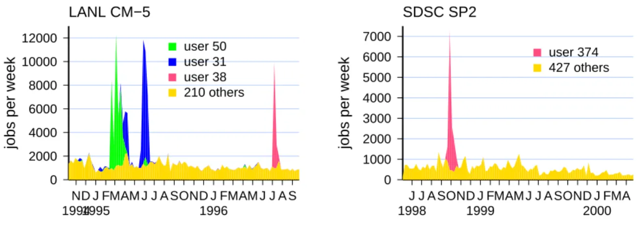
Other types of surprises are also possible. Consider, for example, the data shown in Fig. 3. This shows the level of activity (as measured by the number of submitted jobs) on large-scale parallel supercomputers over a period of two years. While fluctuations are of course expected, these graphs show another type of phenomenon as well: flurries of extremely high activity by a single user, that last for a limited period of time [22]. It is not clear why this happens, but it is clear that it has a significant (and unexpected) impact on the statistics of the workload as a whole. generalizing from this and other examples, there is a good chance that if you look at your computer closely enough, you will find that it is doing strange things that you wouldn’t have anticipated (and I’m not referring to a situation in which it had been taken over by a hacker).
The main problem with surprises is that we never fail to be surprised by them. It is very easy to fall into the trap of assuming that — given that we are dealing with a man-made system — we
LANL CM−5
N 1994
D J 1995
FMAM J J A SOND J 1996
FMAM J J A S
jobs per week
0 2000 4000 6000 8000 10000 12000 user 50 user 31 user 38 210 others SDSC SP2 J 1998
J A SOND J 1999
FMAM J J A SOND J 2000
FMA
jobs per week
0 1000 2000 3000 4000 5000 6000 7000 user 374 427 others
Figure 3: Arrivals per week in long logs of activity on parallel supercomputers exhibit flurries of activity by single users.
know what is going on, and can therefore plan our actions accordingly. But as a scientist, one needs to develop a sense of healthy skepticism. More often than not, we don’t really know enough. And the only way to find out is by looking.
2.4
Modeling
“The important thing in science is not so much to obtain new facts as to discover new ways of thinking about them.”
Sir William Bragg
“Science is built up of facts, as a house is built of stones; but an accumulation of facts is no more a science than a heap of stones is a house.”
Henri Poincar´e
Well-executed measurements provide us with data. Modeling this data is the process that turns them into information and knowledge. The resulting model embodies what we have learned from the measurements about our world. A good model includes definitions of new concepts and effects, and thus enriches our vocabulary and our ability to discuss the properties of the systems we build. Thus modeling transcends the realm of experimentation, and leads into theory.
An important property of good models is simplicity. A good model doesn’t just define new useful quantities — it also leaves out many useless ones. The act of modeling distills the cumulative experience gained from performing experimental measurements, and sets then in a format that can be used as the basis for further progress [14]. In fact, this is also the basis for natural science, where experimental observations are summarized in simple laws that are actually a model of how nature operates.
It should be stressed that finding new models is not easy. The largest obstacle is actually noticing that a new model is needed. It is very tempting to interpret experimental results in the
light of prevailing preconceptions. This runs the risk of fitting the measurements to the theory, rather than the theory to the measurements.
As an example, consider the issue of message-passing in parallel systems. Parallel programs are composed of multiple processes that execute on different processors, and communicate by sending messages to each other. The performance of the message passing is therefore crucial for the performance of the parallel application as a whole. This has led to extensive measurements of different message-passing systems. One result is the emergence of two basic concepts that describe the performance of message passing: latency and bandwidth.
In an informal sense, latency is “how long it takes to get there”, and bandwidth is “how much can flow in a unit of time”. These concepts can be visualized by considering a water hose. The bandwidth corresponds to the diameter (or rather, the cross section) of the hose, whereas the latency corresponds to the water pressure, and hence to the speed with which it propagates. Note that, somewhat counterintuitively, the two may be independent: while we may expect a system with low latency to provide higher bandwidth, it is also possible to have a lot of water flowing at a slow rate, or just a thin jet of water flowing at a high rate.
But the interesting thing about latency and bandwidth is the mindset they imply. Latency and bandwidth are two parameters, and they imply a model that only has two parameters: a simple linear model. In particular, the common model for the time to transmit a message is
time=latency+message length
bandwidth
Given this model, we can perform measurements and find the parameters: simply measure the time to send messages of different sizes, and fit the results to a linear model. The slope then gives the bandwidth, and the intercept gives the latency.
But other approaches are also possible. For example, it is common to measure the latency of a communication system as the time to send a zero-size message. By definition, this is indeed the time needed to get from here to there. But it does not necessarily correspond to the intercept of a linear model, because the behavior of a real system may be much more complex. This goes to show two things. First, the definition of latency of problematic, and different approaches are possible. Second, more sophisticated models of communication systems may be needed. And indeed, several such models have been proposed, including
• The LogP model, which is similar to the simple linear model, but distinguishes between two types of bandwidth: what the network can carry, and what the end-node can inject [11].
• The LogGP model, which adds a separate bandwidth for long messages, that are presumably handled by a different transmission protocol [1].
• The LoGPC model, that adds modeling of network contention [44].
The motivation for all these models is the inadequacy of previous models to describe a real mea-sured phenomenon that is perceived as important. And even more details are needed when the messages are generated automatically in a shared-memory system [43].
One field in which massive data is collected but practically no modeling is attempted is com-puter architecture. Microarchitectural design in particular suffers from immense complexity, with
myriad factors that all interact with each other: instruction mixes, instruction dependencies, branch behavior, working-set sizes, spacial and temporal locality, etc., and also the correlations among all of them. The commonly used alternative to modeling is to agree on a select set of benchmarks, e.g. the SPEC benchmarks, and settle for measurement of these benchmarks. However, this comes at the expense of understanding, as it is impossible to design experiments in which specific char-acteristics of the workload are modified in a controlled manner.
Other fields suffer from the opposite malady, that of modeling too much. In particular, we tend to jump to models without sufficient data, and for the wrong reasons. The prevalence of Poisson models in operating systems and networking is a good example. It is easy to convince oneself that a Poisson model is reasonable; in essence, it amounts to the claim that events happen independently and at random. What could be more reasonable for, say, job arrivals, or component failures? But the fact that it seems reasonable doesn’t mean that this is the truth: more often than not, it just points to our lack of imagination (in this specific example, regarding the possibility that arrival processes are often self-similar and display long-range dependence). The use of Poisson models in the interest of mathematical tractability is even more dangerous, because it may foster a tendency to ignore known data. For example, the earliest measurements of computer system workloads in the 1960s exposed non-Poisson behavior and non-exponential distributions [9, 55, 67], but these were ignored for many years in favor of the mathematical convenience of assuming memoryless behavior.
2.5
Truth
“Errors using inadequate data are much less than those using no data at all.”
Charles Babbage
“Believe those who are seeking the truth. Doubt those who find it.”
Andre Gide
The scientific method is based on the quest for truth by means of objective observations. Ob-viously this is a problematic prospect, and the issue of whether objectivity is really possible has been discussed for hundreds of years. But John Henry writes [32]:
Whether objective knowledge is really possible or not (and sociologists would say it isn’t), it is clearly better to aspire to a knowledge that is free from ideological bias rather than to promote claims to truth that have been deliberately conceived to support a particular ideology or an ungrounded system of belief.
In the quest for objective knowledge, computer science faces a much bigger problem than the natural sciences: the problem of relevance. The natural sciences, as their name implies, are concerned with nature. Nature is unique and enduring, so measurements performed in Paris in the 17th century are valid to London in the 19th century and Calcutta in the 21st century. But measurements of a computer in room 218 may be irrelevant to the computer situated in room 219 at the same time, even if they are of the same model, due to subtle differences in their configuration or use. Results of computer measurements are generally not universal; rather, they are brittle, and
are very sensitive to the conditions under which they were gathered and especially to the specific system being used.
Another problem is the rate of change in the technology-driven realm of computers. Many fea-tures of computer systems grow at exponential rates: the density of elements in integrated circuits (Moore’s law [59]), the size of primary memory, and the performance of and number of processors in typical supercomputers [20], to name a few. Under such circumstances, measurements tend to be short-lived. By the time you manage to perform a measurement and analyze the results, these results may already be out of date, because newer and better systems have emerged.
Of course, not all computer-related measurements necessarily suffer from such problems. For example, some measurements are more closely related to how people use computers than to the computers per se. As such, they only change very slowly, reflecting changes in user behavior (e.g. in 2005 people probably type somewhat faster on average than they did in 1965, because computer keyboards are so much more common — but actually this is a mere speculation, and needs to be checked!).
Moreover, it is also interesting to measure and follow those items that do suffer from brittle relevance. One reason is simply to characterize and understand this brittleness. Another is to collect data that will enable longitudinal studies. For example, data is required to claim that certain properties grow at an exponential rate, and to try and nail down the exponent. A third reason is that while the actual numbers may be of little use, the understanding that is derived from them has wider applicability. Measurements necessarily yield numbers, but these numbers are typically a means and not an end in itself. If we learn something from them, we shouldn’t care that they are not universally correct. If we never measure anything out of fear that it will not be relevant, such irrelevance becomes a self-fulfilling prophecy.
The problem with computer measurement is not that they do not lead to a universal and en-during truth. The problem is expecting them to do so. Even in the natural sciences measurements are qualified by the circumstances under which they were collected. Admittedly, with computers the situation is much more problematic, due to rapid technological change. But partial data is still useful and better than nothing. It is simply a matter of acknowledging this situation and making the best of it.
2.6
Sharing
“One of the advantages of being disorderly is that one is constantly making exciting discoveries.”
A. A. Milne
Getting data is hard. Getting good data is even harder. It is therefore imperative that data be shared, so that the most benefit possible will be gleaned from it. In particular, sharing data enables two important things:
1. Exploration — there is always more to the data than you initially see. By making it available, you enable others to look at it too. Paraphrasing Linus’s Law, with enough eyeballs, the data will eventually give up its secrets.
2. Reproducibility — given your data, others can redo your analysis and validate it. This notion is elaborated in Section 4.
Given that data is hard to come by, it is wasteful to require everyone to get the data anew. In many cases it may even be impossible, as not everyone has access to the measured system. For example, only the operators of a large-scale supercomputer have access to it and can measure its performance and workload. But they are not necessarily the best equipped to analyze this data. It is therefore much more efficient to share the data, and enable others to look at it. Of course, if possible it is highly desirable to get new data too; but the option of using known data is important to enable more people to work on it, and to foster a measure of uniformity across different analyses. Sharing the data is extremely important even if you do perform a detailed analysis. Access to the raw data is required both in order to validate the analysis, and in order to perform new types of studies. It should be stressed that validation is not a sign of mistrust — this is simply how science is done. As for innovative analyses, it can be claimed that this is a highly creative endeavor, maybe even more than the effort needed to collect good data in the first place. For example, consider a workload log from a parallel supercomputer that includes the following data for each submitted job:
• User ID, with indication of special users such as system administrators.
• Application identifier for interactive jobs (with explicit identification of Unix utilities), or an indication that the job was a batch job.
• Number of nodes used by the job.
• Runtime in seconds.
• Start date and time.
This doesn’t look like much, but still, what can you extract from this data? My initial analysis found the following [21]:
• The distribution of job sizes (in number of nodes) for system jobs, and for user jobs classified according to when they ran: during the day, at night, or on the weekend.
• The distribution of total resource consumption (node seconds), for the same job classifica-tions.
• The same two distributions, but classifying jobs according to their type: those that were submitted directly, batch jobs, and Unix utilities.
• The changes in system utilization throughout the day, for weekdays and weekends.
• The distribution of multiprogramming level seen during the day, at night, and on weekends.
• The distribution of runtimes for system jobs, sequential jobs, and parallel jobs, and for jobs with different degrees of parallelism.
• The correlation between resource usage and job size, for jobs that ran during the day, at night, and over the weekend.
• The arrival pattern of jobs during the day, on weekdays and weekends, and the distribution of interarrival times.
• The correlation between the time of day a job is submitted and its resource consumption.
• The activity of different users, in terms of number of jobs submitted, and how many of them were different.
• Profiles of application usage, including repeated runs by the same user and by different users, on the same or on different numbers of nodes.
• The dispersion of runtimes when the same application is executed many times.
While this is a pretty extensive list, I am confident that someone reading this paper will be able to come up with additional interesting observations. If you are interested, the original data is available from the Parallel Workloads Archive. In fact, quite a few repositories of data already exist, including
Internet Traffic Archive at URLhttp://ita.ee.lbl.gov/
NLANR Internet Traces at URLhttp://moat.nlanr.net/
CAIDA Internet Traces at URLhttp://www.caida.org/
MAWI Backbone Traffic Archive at URLhttp://mawi.wide.ad.jp/mawi/
LBNL/ICSI Enterprise Tracing Project at URLhttp://www.icir.org/enterprise-tracing/index.html
Waikato Internet Traffic Storage at URLhttp://www.wand.net.nz/wand/wits/
Video Frame Size Traces at URLhttp://www-tkn.ee.tu-berlin.de/research/trace/trace.html
BYU Performance Evaluation Laboratory traces of address, instruction, and disk I/O at URL
http://traces.byu.edu/
New Mexico State University traces of address references for processor architecture studies at
URLhttp://tracebase.nmsu.edu/tracebase.html
Parallel Workload Archive for workloads on parallel supercomputers at URL
http://www.cs.huji.ac.il/labs/parallel/workload/.
Hopefully, in the future all relevant data will be deposited in such repositories, which will be maintained by professional societies. Regrettably, some of these repositories seem to be dead. For example, the well-known Internet Traffic Archive was set up to provide access to data used in networking and web performance studies, and contains the datasets used in several pioneering papers. But it only contains data collected between 1995 and 1998.
A legitimate issue is the need to get the most out of your hard-earned data before allowing others to get their hands on it, possibly scooping you to the publication of the results. This concern is easily handled by fostering a cultural acceptance of some delay in making the data available. One option is to keep the data private until you publish your own initial results, as is commonly done e.g. in biology. Another option is to wait for a fixed period after obtaining the data, e.g. one year. Deciding on such a fixed timeframe is preferable in that it avoids situations in which the data
is continuously kept private out of anticipation of additional analysis, which never materializes; there are too many cases of researchers who intend to make data available but are then sidetracked and the data is lost.
On the other hand, it can be claimed that the fear of being scooped is actually not well founded. The current situation is that data can lay around for years before anyone bothers to look at it. One of my personal examples is the workload flurries shown above in Fig. 3, which were discovered in widely available (and used) data [22]. Another is the analysis of Top500 data, which is also a well-known and widely cited dataset [19, 20].
Thus the flip side of the argument for keeping data for private exploitation is the opportunity for even more exciting discoveries if you make it public. As the above examples show, it can take many years for someone to come up with a new use for existing data. By making the data public, we increase the chances that someone will have a use for them. This is especially relevant for large scale monitoring projects, that just collect data for no obvious reason. For example, Kumar et al. have used monitors of network address usage to track down the IP address from which an Internet worm was launched [37]. This use was not anticipated when the data collection was initiated, and would not have been possible if the data was not available.
3
Hypothesis Testing
“A fact is a simple statement that everyone believes. It is innocent, unless found guilty. A hypothesis is a novel suggestion that no one wants to believe. It is guilty, until found effective.”
Edward Teller
“Smart people (like smart lawyers) can come up with very good explanations for mis-taken points of view.”
Attributed to an un-named “famous scientist” by Frank Wolfs
Hypothesis testing is at the very core of the scientific method. This is where experimentation comes in. This is where you interrogate nature to see whether what you think you know is indeed true.
As outlined in the previous section, experimental science starts with observation. Based on the measured observations, one builds a model. The model is an abstraction of the world, and embodies a generalization of the results of the measurements; it is an expression of what you have learned from them.
But such a model is a theory, not a fact. How do you know if this is the correct generalization? The model or theory by itself is useless. To justify itself, a model must be used. The way to use a model is to make predictions about the world, and in particular, about aspects that have not been measured yet. Such predictions are actually hypotheses about what the outcome of the missing measurements will be — an educated guess, based on our prior knowledge, but not yet real knowledge in itself.
To turn a hypothesis into bone-fide knowledge, it has to pass the test of experimentation. A special test is designed, which will measure specifically whether the hypothesis makes the right
prediction. This closes the cycle (Fig. 1): a measurement led to a model, the model to a hypothesis, and now the hypothesis is used to guide another measurement. This in turn may lead to a refinement of the model, and so on.
3.1
Emergent Hypotheses
“Wise men profit more from fools than fools from wise men; for the wise men shun the mistakes of fools, but fools do not imitate the successes of the wise.”
Cato the Elder
“Your theory is crazy, but it’s not crazy enough to be true.”
Niels Bohr
The term “hypothesis” is actually quite loaded, and is used at two quite different levels: the macro level and the micro level. The above discussion and the next subsection are focused mainly towards the micro level, where a specific, concrete, atomic prediction is to be tested. But at least some previous discussions of hypothesis testing in computer science has focused on the macro level.
Macro level hypotheses are concerned with the shaping of a whole field, as opposed to the micro level employed in individual research projects. Perhaps the best-known such hypothesis in computer science is that P 6= NP, and thus efficient polynomial algorithms for NP-complete
problems cannot be found. This has led to extensive research on approximation algorithms, and to further classifications of problems according to whether or not good approximations are possible. While we do not know for a fact thatP 6= NP, we accept this hypothesis because it has passed
extensive tests: generations of computer scientists have tried to refute it and failed.
Various subfields of computer science have their own macro hypotheses. As cited above, Newell and Simon propose the hypothesis that intelligent behavior is achieved by heuristic search [47]. Denning suggests that a basic hypothesis in performance analysis is that queueing networks provide an adequate model for making predictions [14]. These hypotheses can be called emergent hypotheses — they are not proposed and then tested systematically; rather, they emerge as a sum-marizing principle that unites a large body of work. The micro-hypotheses discussed next are of the opposite kind, and can be called ad-hoc hypotheses: they are formulated for a specific need, and then tested to see that they fulfill this need.
3.2
Hypothesis-Driven Experiments
“When you have eliminated the impossible, whatever remains, however improbable, must be the truth.”
Sherlock Holmes
“If at first the idea is not absurd, then there is no hope for it.”
0 20 40 60 80 100
0.4 0.5 0.6 0.7 0.8 0.9 1
average bounded slowdown
load EASY conservative difference
-100 -50 0 50 100 150 200 250 300
0.4 0.5 0.6 0.7 0.8 0.9 1
average bounded slowdown
load EASY conservative difference
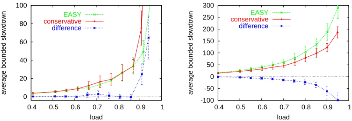
Figure 4: Comparison of EASY and conservative backfilling, using the CTC workload (left) and the Jann model (right).
The micro level of hypothesis testing is concerned with individual experiments and measure-ments. In computer science, just like the natural sciences, we need to explain the results of our measurements. We are interested in some aspect of a computer system. We measure it. And now we have to make sense of the results. This is typically done by trying to explain why the system behaved in the way it did, or in other words, by coming up with a model of how the system behaves, and showing that the model agrees with the measured results.
But what about the other way around? In the natural sciences, it is not enough that the model fit the measurements — it is also required that new measurements fit the model! In effect, the claim that the proposed model explains the system behavior is not a proven truth, but merely a hypothesis. This hypothesis needs to be tested. If it passes the test, and then another test, and another, we gain confidence that the model is indeed a faithful representation of the system’s innermost working. Of course, the tests may also show that our model is wrong, and then we need to seek other explanations.
While the prevailing culture in computer science does not require the experimental verification of hypotheses derived from models, such a procedure is nevertheless sorely needed. We show this by means of a case study (taken from [18]). The case study concerns the comparison of two variants of a scheduler for parallel systems. The scheduler may have some free nodes at its disposal, and maintains a queue of parallel jobs that cannot run yet because sufficient nodes are not available. When a running job terminates and frees some more nodes, or when a new job arrives, the scheduler scans the queue and starts as many jobs as possible. In particular, when a job that cannot run is found, the scheduler does not stop. Instead, it continues the scan in an effort to find smaller jobs that will fit — an optimization known as “backfilling” [40].
The difference between the two variants is small. When backfilling is performed, there is a danger that skipped jobs will be starved. One variant, called “EASY”, counters this by making a reservation for the first queued job. The other, called “conservative”, makes reservations for all skipped jobs. The reservation is made for when enough nodes are expected to be free, based on user-supplied estimates of job runtimes.
workload traced on the IBM SP2 parallel supercomputer installed at the Cornell Theory Center (CTC), and a statistical model of this workload developed by Jann et al. [35]. The performance metric is bounded slowdown: the response time normalized by the actual runtime, but using a value of 10 seconds instead of the real runtime if it was too small, in order to prevent extremely high values when very short jobs are delayed. The results are shown in Fig.4, and indicate a problem: the Jann model is based on the CTC workload, but the results differ. With the Jann model, conservative backfilling is seen to be better. With CTC, they are the same except under extremely high loads, when EASY is better.
In trying to explain these results, we note that both the backfilling policy and the slowdown metric are sensitive to job duration. It therefore makes sense to check for statistical differences between the workloads. The most striking difference is that the Jann workload has tails at both ends of the runtime distribution, which the CTC workload does not.
The long jobs in the tail of the distribution could affect the observed results by causing longer delays to other jobs that wait for their termination because they need their processors. But wait! This is not yet an explanation; it is only a hypothesis about what is happening. To check it, an appropriate experiment has to be devised. In this particular case, we re-ran the simulations with a modified version of the Jann workload, in which all jobs longer than 18 hours were deleted (in CTC, there is an 18-hour limit). However, the results were essentially the same as for the original workload, refuting the hypothesis that the long jobs are responsible for the difference.
The next candidate hypothesis is that the very short jobs in the Jann workload are the source of the observed behavior: short jobs could affect the results by contributing very high values to the average slowdown metric. This was checked by removing all the jobs shorter than 30 seconds. But again, the results were not significantly different from those of the original workload.
Another major difference between the workloads is that in the original CTC workload most jobs use power-of-two nodes, whereas in the Jann model jobs are spread evenly between each two consecutive powers of two. Previous work has shown that the fraction of jobs that are powers of two is important for performance, as it is easier to pack power-of-two jobs [42]. While it is not clear a-priori how this may lead to the specific results observed in the original measurements, it is still possible to check whether the hypothesis that the (lack of) emphasis on power-of-two nodes lies at their base. This is done by running the simulations on a modified version of the Jann workload in which the sizes of 80% of the jobs were rounded up to the next power of two. The experiment yet again demonstrated that the hypothesis is wrong, as this seemed not to make a qualitative difference.
The next hypothesis is that the difference is due to using accurate runtime estimates when simulating the Jann workload, as opposed to using (inaccurate) real user estimates in the CTC workload. If runtime estimates are inaccurate, jobs tend to terminate before the time expected by the scheduler. This creates holes in the schedule that can be used for backfilling. As such holes appear at the head of the schedule, when many subsequent jobs are already queued, this strongly affects conservative backfilling that has to take all subsequent commitments into account. EASY, on the other hand, only has to consider the first commitment. Therefore conservative achieves much less backfilling.
-20 0 20 40 60 80
0.4 0.5 0.6 0.7 0.8 0.9 1
average bounded slowdown
load EASY conservative difference
Figure 5:Results for the CTC workload when using actual runtimes as estimates, to verify that this is the cause of the Jann results.
this is not easy to do [64]. It is much easier to modify the CTC workload, and re-run the CTC simulations using the actual runtimes rather than the original user estimates to control the backfill-ing. The results, shown in Figure 5, largely confirm the conjecture: when using accurate estimates, conservative comes out better than EASY. The hypothesis has therefore passed the test, and can be used as the basis for further elaboration.
While such case studies are not very common in systems research, it should be stressed that they do exist. Another prime example we can cite is the study by Petrini et al. regarding the performance of the ASCI Q parallel supercomputer [53]. This was different from the case study described above, in that it was an empirical investigation of the performance of a real system. A number of hypotheses were made along the way, some of which turned out to be false (e.g. that the performance problems are the result of deficiencies in the implementation of the allreduce operation), while others led to an explanation of the problems in terms of interference from system noise. This explanation passed the ultimate test by leading to an improved design that resulted in a factor of 2 improvement in application performance.
In grade school, we are taught to check our work: after you divide, multiply back and verify that you get what you started with. The same principle applies to the evaluation of computer systems. These systems are complex, and their behavior is typically the result of many subtle interactions. It is very easy to fall for wrong explanations that seem very reasonable. The only way to find the right explanation is to check it experimentally. This is both a technical issue — devising experimental verifications is not easy, and a cultural one: the notion that unverified explanations are simply not good enough.
3.3
Refutable Theory
“If the facts don’t fit the theory, change the facts.”
Albert Einstein
“A theory which cannot be mortally endangered cannot be alive.”
Regarding possible explanations of system performance as mere hypotheses, and devising ex-periments to check their validity, are not only a mechanism for finding the right explanation. Hy-pothesis testing and refutable theory are the fast lane to scientific progress [54].
Using explanations without thinking about and actually demonstrating proper experimental verification may lead us to false conclusions. This is of course bad. But the real damage is that it stifles progress in the right direction, and disregards the scientific method. Platt writes about hand-waving explanations, which are easily reversed when someone notices that they contradict the observation at hand [54],
A “theory” of this sort is not a theory at all, because it does not exclude anything. It predicts everything, and therefore does not predict anything. It becomes simply a verbal formula which the graduate student repeats and believes because the professor has said it so often. This is not science, but faith; not theory, but theology. Whether it is hand-waving, or number-waving, or equation-waving, a theory is not a theory unless it can be disproved.
Platt’s main examples come from the natural sciences, e.g. molecular biology and high-energy physics [54]. The theories he talks about are theories regarding nature: that the strands of the dou-ble helix of DNA separate when a cell divides, that the parity of elementary particles is conserved, etc. But is this also relevant to the computer systems conjured by humans? The answer lies with the basic characteristics of the scientific research that Platt is talking about: that it is observational, and subject to limited resources.
That the natural sciences are based on observing nature is taken for granted. But computer science? After all, we design these systems; so can’t they be analyzed mathematically from first principles? The short answer is no, as we tried to establish above. Whether at the scale of a single microprocessor or of the whole Internet, we don’t really know what our computer systems are doing, and there is no alternative to direct observation.
Perhaps more surprising is the observation that limited resources have a crucial role. Why do limited resources promote good experimental research? Because if you have limited resources, you need to think about how to best invest them, or in other words, what will yield the best returns on your investment. And the answer of the scientific method is that the best return is obtained by carefully designed experiments, and specifically, those that can best distinguish between competing theories. Furthermore, this leads to more collaboration between scientists, both in terms of ferment and cross-pollination of ideas and advances, and in terms of building large-scale experimental infrastructure that cannot be built by individual research teams. These considerations apply equally well to computer science.
Platt ends his exposition with the following recommendation [54]:
I will mention one severe but useful private test — a touchstone of strong inference — that removes the necessity for third-person criticism, because it is a test that any-one can learn to carry with him for use as needed. It is our old friend the Baconian “exclusion,” but I call it “The Question.” Obviously it should be applied as much to one’s own thinking as to others’. It consists of asking in your own mind, on hear-ing any scientific explanation or theory put forward, “But sir, what experiment could
disprove your hypothesis?”; or, on hearing a scientific experiment described, “But sir,
what hypothesis does your experiment disprove?”
4
Reproducibility
“When you steal from one author, it’s plagiarism; if you steal from many, it’s re-search.”
Wilson Mizner
“Mathematicians stand on each other’s shoulders while computer scientists stand on each other’s toes.”
R. W. Hamming
We’re human. We make mistakes. Even in science. So it is beneficial to allow others to repeat our work, both to verify it and to refine and extend it.
4.1
Mistakes
“The greatest mistake you can make in life is to be continually fearing you will make one.”
Elbert Hubbard
“Admit your errors before someone else exaggerates them.”
Andrew V. Mason
“An expert is a man who has made all the mistakes which can be made in a very narrow field.”
Niels Bohr
“If you don’t make mistakes, you’re not working on hard enough problems.”
F. Wikzek
I some fields the propensity for mistakes is well-documented, and accepted as part of life. A prime example is software engineering. Practically all software life-cycle models are based on the notion of iteration, where successive iterations of the development correct the shortcomings of previous iterations [58]. As mistakes are typically found by testing the software, testing has become a major part of development. In the Unified Process, testing is one of four main workflows that span the duration of a software development project [34].
But mistakes happen in all domains of human endeavor, and finding them is a social activity that requires a time investment by multiple participants. De Millo et al. list several illuminating examples from mathematics, where proofs of theorems were later found to be flawed [12]. The history of science has witnessed several great controversies among eminent scholars, who can’t all be right [30].
A recent example closer to computer science is provided by the SIAM 100-digit challenge [3]. The challenge was to compute 10 digits of the answer to each of 10 difficult computational problems. 94 groups entered the challenge, and no fewer than 20 won, by correctly computing all 100 digits; 5 additional teams got only one digit wrong. But still, three out of four groups made mistakes, including groups with well-known and experienced computational scientists.
Moreover, in an interview, Nick Trefethen (the initiator of the challenge) admitted to not having known all the answers in advance. But he claimed that such knowledge was not needed, as it was easy to identify the correct answers from the results: when multiple groups from different places using different methods got the same numbers, they were most probably right. Groups who got a unique result were probably wrong — even if composed of highly-qualified individuals.
The lesson from these examples is that we cannot really be sure that published research results are correct, even if they were derived by the best scientists and were subjected to the most rigorous peer review. But we can gain confidence if others repeat the work and obtain similar results. Such repetitions are part of the scientific process, and do not reflect specific mistrust of the authors of the original results. Rather, they are part of a system to support and gain confidence in the original results, and at the same time to delimit the range of their applicability.
To enable others to repeat a study, the work has to be reproducible. This has several important components [45, 36, 51]:
1. Describe the work in sufficient detail. Think in terms of a recipe that lists all what has to be done, and don’t assume your readers can fill in the gaps. Don’t forget to include trivial details, e.g. whether MB means 106 bytes or 220 bytes. Design and use tools that automatically record full details of the environment in which a measurement is taken [50]. 2. Make software available in a usable form, i.e. source code rather than binaries. This is
especially important for new software you developed for the reported experiment; the more it is used, the better the chance that hidden bugs will be found and removed. If using software produced by others, specify the version used.
3. Make raw data available, especially input data, e.g. the workload used to drive a simulation. 4. Enable access to infrastructure. This may be crucial in certain cases where the infrastructure
is unique, either because of its novelty or because of its pricetag.
Incidentally, keeping all the data needed in order to reproduce work is also very useful when you have to reproduce it yourself, e.g. in a followup study or when revising a paper [51].
4.2
Understanding
“It is by universal misunderstanding that all agree. For if, by ill luck, people under-stood each other, they would never agree.”
Charles Baudelaire
“All truths are easy to understand once they are discovered; the point is to discover them.”