Relay Based Thermal Aware and Mobility Support
Routing Protocol for Wireless Body Sensor
Networks
Maryam el Azhari, Ahmed Toumanari, Rachid Latif and Nadya el Moussaid
LISTI lab, National School of Applied Sciences, Ibnou Zohr University, Agadir, Morocco
[email protected],[email protected], [email protected],[email protected]
Abstract: The evolvement of wireless technologies has enabled
revolutionizing the health-care industry by monitor patient health condition requiring early diagnosis and interfering when a chronic situation is taking place. In this regard, miniaturized biosensors have been manufactured to cover various medical applications forming therefore a Wireless Body Sensor Network (WBSN). A WBSN is comprised of several small and low power devices capable of sensing vital signs such as heart rate, blood glucose, body temperature etc.. Although WBSN main purpose is to provide the most convenient wireless setting for the networking of human body sensors, there are still a great number of technical challenges to resolve such as: power source miniaturization, low power transceivers, biocompatibility, secure data transfer, minimum transmission delay and high quality of service. These challenges have to be taken into consideration when creating a new routing protocol for WBSNs. This paper proposes a new Relay based Thermal aware and Mobile Routing Protocol (RTM-RP) for Wireless Body Sensor Networks tackling the problem of high energy consumption and high temperature increase where the mobility is a crucial constraint to handle.
Keywords: Biosensors, healthcare applications, Mobility, Relay
sensors, Routing Protocols, Wireless Body Sensor Networks.
1.
Introduction
Wireless Body Sensor Networks (WBSNs) is a subtype of Wireless Sensor Networks (WSNs) capable of monitoring medical and non medical applications via multi-hop or single hop topologies. They are characterized by a limited range of transmission and a small number of in-body and on-body biosensors. Several protocols have been proposed to handle packets routing in WSNs [1-2-17-18], however these protocols cannot be directly used in WBSNs since additional constraints are imposed.
The heat generated by antenna and node’s circuitry can damage the human tissue, hence, it is essential to define the biosensor temperature rise as a metric when performing data routing towards the destination [3].
Biosensors have smaller size compared to normal sensors used in WSNs, which implies smaller size of batteries, to put it another way, when a certain amount of energy corresponding to “x” units is consumed within a sensor, the same amount might lead to a complete depletion of the biosensor batteries and therefore reducing the network lifetime.
The human body is characterized by a very high mobility taking different models such as: SITTING, WALKING, LAYING-DOWN, RUNNING etc…this high mobility leads to frequent disconnection between the sender and the receiver minimizing then the efficiency of a particular routing protocol in terms of throughput .
Data priority is a crucial factor that has to be taken into account while implementing a routing protocol for WBSNs for instance ECG and EEG signals have to be delivered in real time compared with other parameters e.g. body temperature or blood pressure [4], so that further decision can be taken instantly especially for persons with critical situation [5].
The rest of this paper is organized as follows: section 2 briefly reviewed routing protocols in WBSNs, section 3 presents the advantages of using relay nodes in WBSNs whereas section 4 features our new proposed routing protocols called RTM-RP .Performance analysis is given in section 4, finally Section 5 concludes this paper.
2.
Overview of Routing Protocols in Wireless
Body Sensor Networks
Implementing a routing protocol for WBSNs can be a nontrivial task to tackle due to its various constraints, for instance, the rising temperature of in/on body sensors can damage the human body whereas the mobility can significantly increase packet loss value. Several protocols has been proposed to address the above mentioned issues and they can be divided into five categories: cluster based routings protocols, thermal aware routing protocols, cross layer based routing protocols, QoS aware routing protocols and delay tolerant aware routing protocols [6] and [7], however none of the above routing protocols has taken into consideration the effect of mobility on routing performance. In [8], authors presented M-ATTEMPT routing protocol which supports mobility and minimizes both the energy consumption and temperature increase. The protocol is based on direct communication for real-time traffic and Multi-hop communication for normal data delivery based on forwarding the packet to the next end point, this concept will highly unbalance the energy consumption throughout the network and minimize its lifetime for the transceiver being on in a
continuous period of time. In the next section, we will be discussing the effect of using relays to improve the performance of routing in WBSNs.
3.
Relay Node Based Wireless Body Sensor
Networks
of transmission /reception compared with normal sensors. Relay nodes cooperate to transmit data to the central device, conserving thus a great amount of energy needed to transfer data to the based station. When a sensor is located far away from the destination, a high amount of power needed to transmit data is required however, when a relay node is added to the transmission process, data packet are handed out to the relay node within its communication range, using a small amount of transmission power. LIMB protocol has been proposed in [10] which supports mobility while staying energy efficient. LIMB protocol considered the use of Full Functioning Devices FFDs as an auxiliary static end point capable of receiving data from sensors and forwarding it back to the destination. However the protocol did not consider saving energy among FFDs for they might also run out of energy after certain periods of time using.
In order to minimize the total network cost, an optimization framework has been proposed by Jocelyne in [11] which investigates the optimal design of wireless Body Sensor Networks by determining the optimal number of relays to be deployed and so is their placement sites. The proposed method consisted of defining a mixed integer linear programming model which has been solved using realistic WBSN scenarios and general topology. The model minimizes both the total energy consumption and the network installation cost while maintaining low energy consumption and full coverage of all sensors. The experiments have been conducted considering the scenario where the body is in a standing position with arms hanging along the side. However the optimal solution found is only optimal for the standing position model as it could be sub-optimal (if not sub-optimal) for other scenarios.
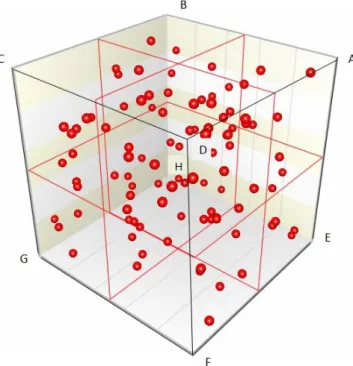
In our work, we improve the proposed optimization framework so that to handle two sets of mobility model which are : static set and mobile set. The static set refers to scenarios where the body is slightly mobile and this includes : SITTING ,LYING DOWN,STANDING ect... whereas the mobile set includes postures where the body experiences a high mobility such as WALKING,RUNNUING ect… To this end,we utilize the configurable mobility for Wireless Body Area Networks named MoBAN [12] in order to determine the coordinates of sensors following a sequence pattern which refers to a sequence of selected postures during a time interval Ts. The distribution of sensor coordinates can be gathered in a cubic form centered on the human body hip and subdivided into eight cubes as depicted in Figure 1. Hence, during a time interval Ts (in minutes),a
sensor node is considered belonging to one of the eight cubes when the body posture is static as it can be included in a maximum of cubes equals to eight when it comes to a mobile posture. After the time interval Ts is passed, each is
affected to where refers to a particular cube vertex,
corresponds to a visited location, and:
Let be a set including all belonging to the vertex . Foreach , we define the centroid where:
refers to the new virtual coordinates of sensor nodes
that is going to be used as input for our new model which consists on developing a non linear optimization problem and resolves it using Knitro Solver[13] coupled with ampl programming language[14], the optimization model is depicted as follows:
(1) s.t.
(2)
(3)
(4)
(5)
(6)
(7)
(8)
(9)
(10)
(11)
(12)
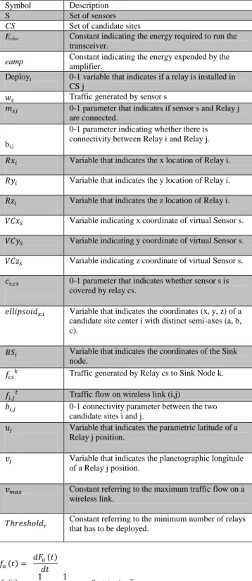
Given the basic notation defined in Table 1, we construct an objective function 1 which aims to minimize the total number of relays deployed and the overall energy consumed by the all biosensors including relay nodes.
term aims to minimize the number of relays deployed in the network so that to guarantee the comfort of the user by carrying a few number of sensors, but also to minimize the total network cost. The term refers to
the total energy consumed by relays to receive data from all sensors. The following two terms:
refers to the total energy consumed in order to send data packets from relays to relays and from relays to sink Node,
refers to the total energy consumed in order to send data packets from relays to relays and from relays to sink Node,
Indicates the total energy consumed by relays to receive data from other relays. Constraint (2) assures that the total traffic received as input to a relay node equals to the total traffic handed out as output to other relays or to sink node. Constraints (3) and (4) verify whether there is a link between two relays. Constraints (5) and (6) determine the definition interval of the parametric latitude and the planetographic longitude of a relay position. Constraints (7) insure that the traffic flow towards a relay node does not exceed a maximum value vmax. Constraints (8)
and (9) insure that a sensor is at least covered by one relay and this relay has to be installed and covering the sensor node. Constraints (10) (11) and (12) set the values of a relay coordinates in accordance with the ellipsoid parameters and finally Constraint (13) ensures that the number of relays to be deployed is at least equals to if not greater.
4.
RTM-RP for Wireless Body Sensor
Networks
In this section, we present our new routing protocol which is relay based and thermal aware routing taking into account the body mobility as a critical constraint to handle but also the priority of data to be sent. In a mobile environment, the link between transmitter and receiver is more likely to be disconnected, for this reason; we define the condition under which the transmitter and the receiver will stay within each other communication range during a time T. This disclaimer will help us decide which relay node within the communication range of a sensor node is more suitable to send data to with minimum data loss.
Figure 1. Distribution of sensor locations corresponding to
the mobile set
4.1 Connectivity condition
Supposedly we have a sensor node N capable to communicate with relays: , and as shown in Figure2.
Figure 2. Illustration of a sensor N capable to communicate
For simplicity reasons, we consider sensor N as immobile whereas relays are changing their destinations randomly. In order for sensor N to maintain connectivity to , the distance between sensor N and the new position of has to be inferior if not equals to during time interval T where
is the communication range of sensor N and , corresponds to the time required to move from position
to and x ϵ N (see Figure 3) .
Figure 3. Illustration of possible relay positions during time T.
This condition is articulated as follows:
(14)
Let’s consider the case where a relay is changing its position from to P2 as depicted in Figure 3, indicates the initial distance between N and such as:
is a random variable that can be defined as the
distance between two random points in a box with sides a, b and c. The problem of the average distance points between two random points in a box was treated by so many authors D.P.Robins, T.S.Bolin, and E. Weinstein [15].
In [10], Johan Philip determined the probability distribution for the distance between two random points in a box with sides a, b and c. The average of this distance is known before as Robbins’s constant. Johan’s method consisted in determining the distance distributions for each of the three directions x, y, z and convolve them to retrieve the distribution of .
Let and be two random points in a space with the
following coordinates respectively: and
where x, y and z are distributed in the intervals (0, a), (0, b) and (0, c) and each ( and ( ) pair of coordinates is independent, also the box
sides satisfy .
The following distribution and density functions were defined:
The probability density for the event as
depicted in Figure 4 is:
Table 1. Basic notation Symbol Description
S Set of sensors
CS Set of candidate sites
Eelec Constant indicating the energy required to run the
transceiver.
eamp Constant indicating the energy expended by the
amplifier.
Deployj 0-1 variable that indicates if a relay is installed in CS j
Traffic generated by sensor s
0-1 parameter that indicates if sensor s and Relay j are connected.
bi,j
0-1 parameter indicating whether there is connectivity between Relay i and Relay j.
Variable that indicates the x location of Relay i.
Variable that indicates the y location of Relay i.
Variable that indicates the z location of Relay i.
Variable indicating x coordinate of virtual Sensor s.
Variable indicating y coordinate of virtual Sensor s.
Variable indicating z coordinate of virtual Sensor s.
0-1 parameter that indicates whether sensor s is covered by relay cs.
Variable that indicates the coordinates (x, y, z) of a candidate site center i with distinct semi-axes (a, b, c).
Variable that indicates the coordinates of the Sink node.
Traffic generated by Relay cs to Sink Node k.
Traffic flow on wireless link (i,j)
0-1 connectivity parameter between the two candidate sites i and j.
Variable that indicates the parametric latitude of a Relay j position.
Variable that indicates the planetographic longitude of a Relay j position.
Constant referring to the maximum traffic flow on a wireless link.
Constant referring to the minimum number of relays that has to be deployed.
The probability density for the event −1 2≤ is defined as the convolution g of .
The density function g is therefore taking three values based on and domains of definition.
When a = b, the expression of g is reduced to the expression below:
The distance between two random points in a rectangle is equivalent to:
Figure 4. Illustration of the area Fa(t)
The expected distance equals to:
For a=b=1
Bolis defined in [3] the expected distance between two points in a box by splitting it into three identical cones with sides: 2a, 2b, and 2c.The integral was applied to a cone in spherical coordinates. The result is defined as follow:
For a=b=c=1 and
Bolis defined in [3] the expected distance between two points in a box by splitting it into three identical cones with sides: 2a, 2b, and 2c.The integral was applied to a cone in spherical coordinates. The result is defined as follow:
For a=b=c=1 and
Based on Bolis result, we defined as been the
average distance between in a box with side’s value equals to 1. In the following, we will be referring to
as S. The expression (14) becomes then:
Based on (15) , we define the maximum distance between N and that insures link connectivity during time as follows:
Let and be:
Then:
The maximum value of equals to:
Three cases have to be treated:
Case 1
Let
Thus:
In order for a sensor node to be connected during the interval T, the following condition has to be satisfied:
where:
and and
Case 2
Where Cte is a constant equals to:
Cte =
In order to insure connectivity between and during the interval T, the following expression has to be satisfied:
where:
and and
Case 3
Similarly to case 2, we define the connectivity condition as:
where:
and
Let’s consider the following notations:
A:
B:
Based on the results above, a relay is chosen when the maximum number of intervals during which a sensor node is connected to a relay node converges to x. For each relay, we compute such as:
4.2 Temperature increase model
In order to represent the temperature increase model of a biosensor, the simulation time is composed of successive sub-intervals ∆t where ∆t has to satisfy the two conditions:
and
The sensor transceiver consumes a great amount of energy due to transmission and reception .We present in the energy consumption model which is composed of energy of transmission , energy of reception and the energy consumed in sleeping mode . and are two linear functions where .
As shown in Figure 5, a certain amount of energy is consumed during which equals to:
Our purpose is to define the temperature increase unit
based on the energy consumed during , for this reason, we define as:
where
During sensor functioning time, is gradually increased
(unless the sensor is in the sleeping mode) until a temperature threshold is reached, the sensor will then turn off the transceiver and stay inactive for which is the
time needed for the sensor to cool down.
Figure 5. Energy consumption during simulation time T
4.3 RTM-RP mechanism
Our new Relay based Thermal aware and Mobile Routing Protocol offer a flexible superframe that can be adjusted depending on relays buffer size. As shown in Figure 6, the superframe starts with a Radom Access Period (RAP) during which sensors send their data to the end point in respect to their priority using Slotted CSMA mechanism. In our case, an end point might refer to the hub or to relay node. The RAP phase is then followed by Relay Buffer TDMA which size is variable and depends on the number of deployed relays, during this period, relays will exchange buffer information to other relays using TDMA minislots. TDMA scheduling can be provided as a set up parameter as is can be based on relays priorities. In Relay DATA TDMA phase, relays will be sending data packet to the hub based on the buffer information received from other relays via one or multiple TDMA slots.
Figure 6. RTM-RP superframe structure.
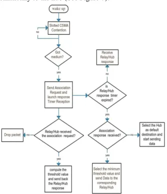
As illustrated in RTM-RP flow chart (Figure 6), the super frame starts by waking up all network sensors, by default, we consider the hub and relays awake and set to reception state. At the beginning of RAP Slotted CSMA phase, sensors contend to access the channel using Slotted CSMA mechanism. A node with high priority is more likely to gain medium access, when it is the case; the sensor node will broadcast an association request destined to all relays and hub in the vicinity and launch a timer for relay (or hub) response reception. In meanwhile, relays (or hub) receiving the association request will calculate and send back the threshold parameter value to the sensor node. The threshold parameter is defined as follows:
where:
is the sum of temperature increasing units.
RSSI is the Received Signal Strength Indicator.
refers to the sensor remained energy.
is the maximum number of intervals
during which a sensor node will be connected to a relay (or hub).When relay (or hub) response timer is expired, the sensor node chooses the relay (or hub) with minimum threshold value and start sending data packets to it, however when no response has been received, data is transmitted automatically to the hub (See Figure 7).
Figure 7. RAP Slotted CSMA flow chart.
Figure 8. Relay Buffered TDMA flow chart. During Relay DATA TDMA phase, relays will be sending buffered data in the following estimated slot number:
where:
is the time required to send data which basically equals to
the time needed to send one packet multiplied by the number of packets, is the slot length and MAX_ refers to maximum number of data parquets that can be sent by one relay during Relay DATA TDMA phase.
The slots number equals to if
data to be sent is superior to MAX_ and
otherwise. The starting slot depends
mainly on priorities of buffered data which defines afterwards the priority of a relay to access the channel, if many relays happen to have same priority then contention mechanism is taking place at the beginning of the first time slot affected to relays. After sending data packets to destination, relays will turn to sleep mode for the rest of the Relay DATA TDMA phase period, thus an important amount of energy is saved throughout the hall process of transmission (see Figure 9).
Figure 9. Relay Data TDMA flow chart.
4.4 RTM-RP Performance Evaluation Results
We performed our simulation in Castalia 3.3 OMNET++ based simulation framework [16] which is basically designed for WBASNs. We used three metrics to evaluate the efficiency of RTM-RP, cluster based and tree based routings protocols respectively which are: energy consumption, throughput and latency. We started off our simulation by determining the optimal relay coordinates in respect to a particular posture pattern defined within MoBAN mobility model designed to evaluate intra and extra-WBAN communication. The model implemented different postures but also individual node mobility within a particular posture [12],The model code can be accessible through [20] as an add-on to the mobility framework of OMNET++.In our work, we choose a posture pattern composed of the two scenarios : WALKING and RUNNING. The posture pattern can be extended to include other preexisting scenarios such as LYING-DOWN,SITTING, etc., or new scenarios defined by the user and included in posture file with reference coordinates ,radius, speed and other parameters .Moreover, a Markov model can be utilized to model pattern sequences while maintaining the randomness of posture selection, however for the sake of results clarity and precision, we decided to run intensive simulation on the posture pattern : WALKING and RUNNING. The XML file for posture specification can be found in [19], and the resulting virtual sensor nodes coordinates are presented in Table 2.
Table 2. Virtual sensor nodes coordinate
V C1 VC2 VC3 VC4 VC5 VC6 VC7 x 35.59
11 21.98 1
19.7072 22.02 26
35.56 47
32.55 07
20.01 22 y 17.53
96 20.93 58
30.8815 20.87 18
15.17 83
27.26 13
28.99 49 z 7.787
27 7.804 04
7.79321 6.702 37
6.684 89
6.718 68
6.701 98
After defining the centroid coordinates value which are considered as the new virtual location of the sensor nodes, we proceeded to resolve the optimization problem of finding the optimal position of relay nodes using ampl programming language, knitro server and the precalculated virtual sensor nodes coordinates .The optimal relay nodes coordinates and the initial simulation parameters are presented in Table 2 and Table 3. We considered 12 sensors located on a human body in a standing position where the transmission power of sensors in cluster based and tree based routing protocols are set to -10dBm ,the same value is given to relays in RTM-RP routing protocol whilst sensors are set to -25dBm, and the reason for that is to reduce the heating effect caused by the body being exposed to radiation while maintaining the connectivity to relays e.i. hub. The number of relays varies from 3 to 5 and they are deployed in respect to the coordinates computed via our optimization model, we also consider △tu; △tcooling and △Eu equal to : 10s; 20s and 3:1mw
respectively whilst Er, Et and Es values are defined in
Figure 10. Energy consumption
Figure 10 shows the energy consumption of cluster based, tree based, and x-Relays based routing protocols where
.Both cluster based and tree based routing
protocols experiences high energy consumption compared with x-Relays based routing. The pair (Emin; Emax) takes the
following values (in mw) : (0.53; 0.62) for cluster based routing, (0.52; 0.62) for tree based routing, and (0.16; 0.51) for x-Relays routing protocol. Our proposed protocols outperforms both cluster based and tree based routing in terms of energy consumption since it is based on reducing power of transmission and turning the transceiver off when not in use, thus sensors batteries will last longer and the network lifetime is increased to the maximum which explains the results found above.
Figure 11. Application latency in ms Figure 11 shows the average end to end delay of cluster, tree, and x-Relays based routing protocols, as can be observed, 13.4 of cluster based routing packets are received with latency inferior to 100ms, whereas tree based and x-Routing based routing protocols packets are received in various time intervals, for instance, tree based routing receives a high amount of packet within [0,100] and [500,600] ms whilst x-Relays based routing packets reception time is mainly included in [100,200], [200,300] and [300,400] ms with small portion equals to 7.4 in [500,600] versus 91.6 for tree based routing. Once again, our proposed protocol shows a better performance when it comes to packet delay as it insures that packets are sent towards the destination even though the association packet is lost in a way, thus, once the hub is within the sensor communication range, the packet is successfully delivered increasing though the amount of packet received with minimum latency.
Table 3. Optimal relays coordinate in respect to the deployed
relay number
R1 R2 R3 R4 R5 Three
relays
x 23,4477 21,6344 7,7159 - -
y 23,3461 22,1493 7,3724 - -
z 23,3206 21,7390 7,4782 - -
Three relays
x 22,9773 22,9967 22,9654 23.1253 -
y 20,3125 19,9415 19,9020 20,2421 -
z 7,7319 7,3764 7,20102 7,4727 -
Five relays
x 23,5466 23,4644 23,5857 23,4939 23,7106
y 20,4054 20,4599 20,1302 20,1107 20,5568
z 7,6156 7,6919 7,4345 7,1163 7,4620
Figure 12. Throughput of cluster_based and x-Relays
Figure 12 and Figure 13 depict the throughput of the three protocols which is defined as the ratio of packets received by the hub out of all packets sent by sensor nodes. The throughput value is considered as a good indicator when it converges to 1,however when it falls down to 0 or when it is above 1, the protocol is considered as having a worse performance in terms of throughput. As can be observed, cluster based and tree based routing protocols show a very low throughput as it equals to 0.014 as a maximum value for cluster based routing versus 30 for tree based routing protocols whilst x-Routing based routing presents a better throughput as it reaches a maxi-mum value equals to 0.242 when 3 relays are deployed.
and enhancing the number of packets being collided due to the absence of synchronization.
Figure 14. Average received data packets by relay nodes
Figure 14 illustrates the average data packets received by relays when the deployed relay number equals to: 3, 4, and 5. The results obtained proves the absence of correlation between the number of relays and the average data packets received as the maximum value reaches 635 when only 3 relays are deployed versus 180 in case of 5 relays and this is due to the high mobility of sensors e.g. one (or more) relay might be out of sensors communication range along several superframes in accordance with the mobility model, therefore when it comes to a high mobility environment, the number of relays should be reduced to the minimum in such a way that the total network cost is minimized while guaranteeing the comfort of the patient.
5.
Conclusions
In this paper, we proposed RTM-RP routing protocol to handle temperature rise and high mobility beside minimizing the overall energy consumed using relay nodes within biosensors in WBSNs, we also defined an optimization model to find the optimal number of relays to be used and their corresponding coordinates. The results proved the effectiveness of RTM-RP routing protocols in terms of energy consumption, end-to-end delay, and throughput compared with cluster based and tree based routing protocol . The performance of RTM-RP can be improved by taking into account various mobility scenarios which will enhance the accuracy of the virtual sensor locations, also the cubic form centered on the human body hip can be subdivided into more than eight cubes leading to new optimal relay nodes coordinates, thus our RTM-RP presents much more flexibility in terms of the input parameters and it can be adjusted depending on the application type in use.
References
[1] C. Li, H. Zhang, B. Hao . “A Survey on Routing Protocols for Large-Scale Wireless Sensor Networks”, Sensors, Vol.11, No.4, pp. 3498-3526, 2011.
[2] X.Liu, “A Survey on Clustering Routing Protocols in Wireless Sensor Networks”, Sensors, Vol.12, No.8, pp. 11113-11153, 2012.
[3] Oey, C.H.W., Moh, S, “A Survey on Temperature-Aware Routing Protocols in Wireless Body Sensor Networks”, Sensors 2013, Vol.13, No.8, pp.9860-9877, 2013.
[4] Y. Hao,R. Foster, “Wireless body sensor networks for health-monitoring applications,” Physiological Measurement, Vol.29,No.11,pp.1-42,2008.
[5] V. Balasubramanian, "Critical time parameters for evaluation of body area Wireless Sensor Networks in a Healthcare Monitoring Application”, Intelligent Sensors, Sensor Networks and Information Processing (ISSNIP), 2014 IEEE Ninth International Conference ,Singapore, pp. 1-7,2014,
[6] J.I Bangash, A.H. Abdullah, M.H Anisi, A.W. Khan, “ A Survey of Routing Protocols in Wireless Body Sensor Networks”, Sensors, Vol.14, No.1, pp. 1322-1357, 2014. [7] H.B. Elhadj, “A survey of routing protocols in wireless body
area networks for healthcare applications”. International Journal of E-Health and Medical Communications, Vol.3, No.2, pp.1–18, 2012.
[8] N. Javaid, “M-attempt: A new energy-efficient routing protocol for wireless body area sensor networks”. The 4th International Conference on Ambient Systems, Networks and Technologies (ANT), Canada, pp.224–231, 2013.
[9] A. Vallimayil , K. M. Karthick Raghunath, V. R. Sarma Dhulipala and R. M. Chandrasekaran, “Role of relay node in wireless sensor network”, 3rd International Conference on Electronics Computer Technology (ICECT), Kanyakumari, pp. 160–167, 2011.
[10] B.Braem, P. De Cleyn and C.Blondia, “Supporting mobility in body sensor networks. Body Sensor Networks”, 2010 International Conference on Body Sensor Networks, pp.52–55, 2010.
[11]J. Elias, “Optimal design of energy-efficient and cost-effective wireless”,Ad Hoc Networks, Vol.13, pp.560–574, 2014. [12]M. Nabi, M. Geilen, T. Basten, “MoBAN: A configurable
mobility model for wireless body area networks”, the 4th International ICST Conference on Simulation Tools and Techniques, Spain, pp.168-177, 2011.
[13]R.H Byrd, M.E. Hribar, J. Nocedal, “An interior point algorithm for large scale nonlinear programming”, 1997. [14]R. Fourer, D.H. Gay and B. Kernighan, “AMPL: A
Mathematical Programming Language”, Algorithms and model formulations in mathematical programming, pp.150– 151, 1989.
[15] J. Philip, “The Probability Distribution of the Distance Between Two Random Points in a Box”. 2007.
[16]D. Pediaditakis, Y. Tselishchev, A. Boulis, “Performance and scalability evaluation of the castalia wireless sensor network simulator”, Proceedings of the 3rd International ICST Conference on Simulation Tools and Techniques ,spain, pp. 53:1-53:6,2010.
[17]F. Frattolillo, "A Deterministic Algorithm for the Deployment of Wireless Sensor Networks", International Journal of Communication Networks and Information Security, Vol.8, No.1, 2016.
[18]J.Shobana, B.Paramasivan, "A Deterministic Algorithm for the Deployment of Wireless Sensor Networks", International Journal of Communication Networks and Information Security, Vol.7, No.2, 2015.
[19]http://mixim.sourceforge.net/doc2.1/MiXiM/doc/neddoc/proje ctdoc.html.