Interactive long wave spectrum for the thermo dynamic model

e

l-í,

157

Atm6.fera (1988), 1, PP. 157·172

Interactive long wave spectrum for the thermodynamic model

RENE GARDUÑO and JULIAN ADEM*

Centro de CiencilU de /a Atm6.fera, Univer3Ídad NClCionCli Aut6nomll de México, 0..510, Mizico, D. F., MEXICO

(Manuscript received February 25, 1988; in final form June 1, 1988)

RESUMEN

El espectro analítico de absorción de Smith (1969) para la atmósfera se incorpora en un modelo termodinámico.

Esta formulación radiativa, que se aplica a la onda larga, calcula por separado la ab80rtividad por bióxido de carbono y por vapor de agua, como función de la presión, la temperatura y el contenido de ga8 en la atmósfera, y lo hace con alta resolución en longitud de onda.

El agua precipitable o contenido de H 2 0 se calcula, u8ando la fórmula de Adem (1967), como función de variables evaluadaa en el modelo: la temperatura superficial, la temperatura de la troposfera media y la extensión horizontal de la nubosidad.

Con este enfoque el modelo puede simular el efecto de retroalimentación positiva debido a la opacidad infrarroja del vapor de agua; es decir, su efecto invernadero.

El espectro calculado para los valores actuales de las concentraciones de CO2 y H20 concuerda bien con la8 estimaciones de Goody y Robinson (1951), Goody (1954) y Fleagle y Businger (1963).

ABSTRACT

Smith'8 (1969) analytical absorption spectrum of the atmosphere Í8 incorporated in a thermodynamic mode!.

Thi8 radiative formulation is applied to the infrared region. It computes 8eparately the ab80rptivity by carbon dioxide and by water vapor, with a high wave length re80lution, a8 a function of atm08pheric pressure, temperature and gas contento

The precipitable water or H20 content i8 computed using Adem's (1967) formula &8 a function of variables evaluated in the model: the 8urface temperature, the mid-tropospheric temperature and the horizontal extent of c1oudiness.

With this approach the model is able to simulate the positive feedback effect by long wave opacity of water vapor; that is to say its greenhouse effect.

The computed spectrum for present values of CO 2 and H 2 0 concentrations shows good agreement with the estimates of Goody and Robinson (1951), Goody (1954) and Fleagle and Businger (1963).

1. Introduction

In a recent version of Adem's thermodynamic model (Adem and Garduño, 1982, 1984) we used an atmospheric absorption speetrum, constructed by assuming that, for long wave radiation, the atmosphere:

i. behaves as a black body (that is, wholly opaque) in the wave length intervals (0,8¡.tm) and (18¡.tm, 00),

ii. has a window in the interval (8, 12 ¡.tm) and,

iii. between 12 and 18¡.tm, behaves according to the C02 contentj we assume that in this interval the only atmospheric component which absorbs is the C02; its 15¡.tm band is approximated by six steps of _{l¡.tm wide, whose height (absorptivity) is a function of the CO 2 content} and is determined using the results of Yamamoto and Sasamori (1958, 1961) who computed curves of absorptivity against frequency, and gas content, for different values of pressure and

temperature.

This parameterization of the infrared spectrum allowed us to vary the CO 2 content in the modeled atmosphere and simulate its greenhouse effect. In previous papers we applied this approach to evaluate the climate alteration induced by doubling the atmospheric C02 concentration (Adem and Garduño, 1982, 1984).

In such numerical experiments we did not take into account the effect on the absorptivity of changes in atmospheric pressure and temperature during the CO 2 doubling process. This effect seems to be small (Yamamoto and Sasamori, 1958, 1961). Furthermore, we had assumed that H20 do es not emit radiation in the interval (12, 18 ¡.tm), and has a fixed spectrum during the whole experimento

The purpose of this paper is to introduce Smith's (1969) formula to parameterize the long-wave spectrum, in order to introduce a variable emission by H 20 from 12.5 ¡.tm on, besides taking the C02 radiatively active in the interval (12.2, 19.8 ¡.tm). In this approach, the spectrum is computed analytically by means of an empirical formula deduced by Smith (1969), which gives absorptivity as a function of gas content, and equivalent temperature and pressure, defined as vertical averages weighted with the gas distribution in the atmosphere. Furthermore Adem (1967) derived a method, not incorporated in his model up till now, to evaluate the amount of precipitable water in the atmos­ phere using climate variables computed in the model: the surface temperature, the mid-tropospheric temperature and the horizontal amount of cloudiness.

Using together both parameterizations, Smith (1969) for the spectra and Adem (1967) for precip­ itable water, we are able to generate in the model the interaction between atmospheric water vapor and climate, via long wave radiation.

Other authors have dealt with the water vapor problem in a different way. Manabe and Wetherald (1967) assume that the climate system keeps constant the relative humidity of the atmosphere. They also fix the cloudiness. In a later paper Manabe and Wetherald (1975), assuming fixed cloudiness, incorporate a hydrological cycle and an interactive lapse rateo As for long wave radiation, they use gray spectra, interactive with climate, and applied to a multiple-layer atmosphere.

Ramanathan (1976) uses an infrared band spectrum, Le., with sorne resolution in wave length. His model has also many atmospheric layers. The model of Cerni and Parish (1984) uses a gray spectrum and many layers. Liou (1980) gives formulas for both options: gray and band spectra.

Paltridge (1974), Sellers (1973, 1976), Petukhov (1974) and Sergin and Sergin (1976) incorporate in their models partial hydrological cycles.

For an exhaustive list of models and their features, refer to the very complete and up to date Schlesinger's (1984) review.

2.

Sm bar are

ca

wh

Po

mE

T

o

fOI

th4

(1

at m

w

g

INTERACTIVE LONG WAVE SPECTRUM FOR THE THERMODYNAMIC MODEL 159

tnd

val ed

nt

=d Id

d

s

2. AnaIytical spectrum

Smith (1969) fitted experimental based transmission data of the 15¡.tm C02 and rotational H20 bands with a polynomial formula. The spectral variable is the wave number (n) and the coefficients are determined with 5 cm-1 resolution. The validity intervals of the formula are (505, 820 cm-1) for C02 and (200,800 cm-1) for H20. The formula for the H20 absorptivity is

ToU P T

a = 1 - exp{ -exp(Oo

+

01lnTUo

+

02 ln Po

+

03 ln To

+

ToU P ToU T 2ToU 2ToU T P 2 T

C4ln

TUo In Po

+

CslnTUoInTo

+

C6ln TU o

+

C7ln TU In o To

+

°sln Po In T )} o (1)

where a is the fractional absorptivity, P the pressure, T the (absolute) temperature, To = 273K,

Po = 1013 mb and Uo = 1 cm, U is the gas content (also called optical mass or path length), which is measured in cm as the thickness of the gas when it is liquid at STP conditions, namely at temperature

To and pressure Po. For H20, U is the precipitable water. The formula for C02 is similar to the one for H₂0, and it is obtained from (1) by substituting the terms with the coefficients 07 and Os by the following expression

2ToU P ToU 2 T

071n - - l n -

+

0sln--In - .

(2)

TUo Po TUo To

The coefficients C_i (i = 0, ... ,8) depend on the gas and the wave number, and are given by Smith (1969) for H20 and CO2 •

About the application of formulas (1) and (2) to an environment inhomogeneous in T or P (as the atmosphere), these variables should be taken with their equivalent values, defined as the weighted means with respect to the gas content through the layer thickness:

- foU TdU

T=~..---_U (3)

fo dU

U

P = fo PdU

(4)

foU dU

where the superimposed bar indicates the equivalent value, dU is the differential of gas content, and

(5)

In the next sections we will evaluate the integrals in (3), (4) and (5) in the tropospheric layer. We will use the same vertical distributions of temperature and pressure, as Adem (1962), which are given by the formulas:

T = Ta - {3z (6)

{3z)'Y

P=Pa(1 - -

_T

(7)

where T and Pare the values of temperature and pressure at height z (upward coordinate with origin at the Earth's surface, taken as sea level), Ta and Pa are, respectively, the values of T and P

at z

=

O; '1

= g/

R(3 where (3 is the lapse rate, 9 the acceleration of gravity and R the gas constant of the airo We don't take into account orography, therefore, the bottom of the troposphere is taken at the sea level. This level is indicated with subindex a.

In these computations we will deal only with typical values, Le., global and annual averages of the variables: Ta

=

288K, Pa

=

Po, h

=

9 km, (3

=

6.5K km-1, 9

=

980cm s-2, R

=

2.87x106cm2s-2K-1.

When both gases absorb in the same wave number, the net absorptivity is computedassuming that their transmissivities should be multiplied (Smith, 1969). Then the combined absorptivity is

(8)

where A refers to H 20 and B to CO2.

The parameterization of the long wave radiation used previously (Adem, 1962, 1982; Adem and Garduño, 1982) has the wave length

(A)

as spectral variable, while Smith (1969) uses the wave number (n). Both variables are related by

nA = 1. (9)

Therefore, it is necessary to transform Smith's spectrum from the variable n (in cm-1) to A (in

J-Lm). In order to accomplish this, we divide the n coordinate equidistantIy in A; commonly by

intervals of 1 J-Lm, as is used in themodel. Of course, according to (9), each interval has a different number (not integer, in general) of 5 cm-1 (Smith's resolution) steps.

Initially we compute the absorptivity as a function of n by means of formula (1) and expression (2), from 5 to 5 cm-1; then we get the value of a in each 1J-Lm wide interval in A as simple average of the corresponding 5 cm-1 step values that enter in the 1J-Lm interval; the value of a step that enters incomplete in the interval is taken proportional to the fraction included.

3. C02 Pararneters

According to EIsasser (1940) the amount of water vapor aboye approximately the 300 mb level is negligible small. Therefore, it is realistic to assume that the effective radiation temperature of the upper boundary of the model's atmospheric layer is at about this level. For this reason we use as the hight of the layer a value h

=

9 km, and the corresponding pressure P_h

=

307.3 mb. Therefore, we will compute the atmospheric long wave spectrum taking into account only the C02 contained in the modeled layer of hight h. This amount will be denoted UB'

Smith (1969) assumes that the vertical distribution of CO2 is homogeneous in pressure, namely

dUB

(10)

dP =c

where e is a constant. Then

(11)

wh

]

lay

I the

j

181

l lay€

whe

1

4. ] The

wheI

161

INTERACTIVE LONG WAVE SPECTRUM FOR THE THERMODYNAMIC MODEL

where Pa and Ph are the values of the pressure at the surface and at the height h1 respectively.

In order to compute the equivalent pressure (P_{B )} for the CO2 contained in the modePs tropospheric

layer1 we use (10) in formula (4) and include only this layer. The result is

PB = Pa

+

Ph ₍₁₂₎

2

For the total atmospheric CO₂ content (UB ) we assume the value 260 cm₁ which is very close to T

the value used previously (Adem and Garduño1 19821 1984).

As UB is contained between Pa and Ph, and UB_T between Pa and O, according to (10): UB = 181.1 cm. Therefore from (11) and (12), e = 0.2567 cm mb-1 and PB = 660.15 mb1 respectively.

Using (6), (7) and (10) in formula (3), and evaluating the integrals in the modePs tropospheric layer, we get the equivalent temperature of the CO₂

(13)

where a

=

R(3/g

=

1/"1.

Therefore, T B = 263.43 K.

4. Precipitable water

The amount of precipitable water or H20 content in the layer of hight h is given by

(14)

where uAT (T) is the vertical distribution oí H₂0 content as a function of the temperature.

Adem (1967) derived a formula to evaluate UAT (T), which is the following:

(15)

where

R _

0 ­

0.622 R(3

1

T

a

al = --(Al

+

2A2-)

The constant

a',

_{b' ,}

e',

d', g¡, A, Al, A ₂ and B are empirical parameters (Adem, 1967), which Ti: come from c1imatology and laboratory; sorne of them depend on the season, but here we deal only _No

with typical values; i.e., annual averages. Their values are: _{in th,}

a'

= 1.252x107gr s-2 cm- l _Frc

b_'

=

-1.997x105gr s-2 cm- 1K-l

e' = _{1.196gr s-2 cm-} 1_{K- 2}

d' = -3.19gr s-2 cm-1_K-3

gl = 3.2xlO-3gr s-2 cm- 1K-4

Fr(

A = 0.4518

Al = -8.23xlO-7cm-l 2 A2 = 5.5xlO-l3cm­

Su1 B =0.5.

Formula (14) with UAT (T) given by (15), shows that UA is a function of Ta , _{T h, {3} and f; besides, according to (6), {3 = (Ta - Th)/h.

Using observed normal values of T_{a ,} Th, f and h, Adem (1967) computed the Northern Hemisphere

distributions of UA for winter and summer and compared them successfully with the observed cor­ responding values.

6. N

Formula (14), gives UA as the mass of water contained in an atmospheric column with a base of

a) N(J unit are a; then, in cgsK system its units are gr cm-2. An alternative method is to me asure UA as

the volume, which the water contained in the same column would occupy if it were liquid at STP As ba conditions, divided by the unit area; in this case units of UA are cm. Since STP density of liquid _Usi water is Pa = 19r cm-3 both methods to measure precipitable water are numerically the same in _contel cgsK system. We prefer UA in cm.

To

Ó. H ₂0 parwneters

The vertical distribution function of H20 content can be expressed as a function of z, T or P. This

where distribution is defined as

U for dr:

UA

(r)

= dd A (16)

r r

where r is z, T, or P,

uAr(r)

is the vertical distribution of H 20 expressed as a function of r, and dUA _{is the element of H 20 content between coordinate leveis} r and r

+

dr, corresponding to UA and

where UA

+

dUA, respectively.

used a From (16) in order to change the variable of UAT(T) from T to z, it is necessary to multiply the

latituc

second member by ~~. Therefore, _{this pI}

give q

(17)

latituc Obser' Using (6) we obtain:

In F

INTERACTIVE LONG WAVE SPECTRUM FOR THE THERMODYNAMIC MODEL 163

e

r-Df a.s 'P id in

bis

l6)

~nd

md

the

(18)

This is negative because UA decreases with z.

Now we will compute the equivalent temperature (T A) and the equivalent pressure

(P

A) for H20 in the model 's tropospheric layer.

From equation (3) and (16), with r = T we obtain

(19)

where UA is given by (14).

From (6) and (7) we get

P =

Ph(~)7.

T

h

(20)

Substituting (20) in Eq. (4) and using (16) with r = T we obtain

-_{P A} __- Pa

h

TlI ₇

- - 7 T uA_T (T)dT.

UATa TI. (21)

6. Nu:rnerical experi:rnents

a)

Normal vertical distribution 01 atmospheric H₂0

As basic normal values for present conditions we take f" = 0.5 and T_{a ,}

f3

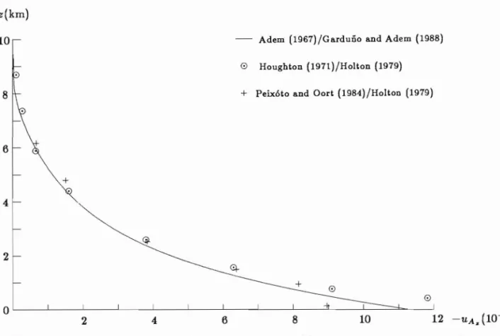
and h as used in section 2.

Using these values in formulas (15) and (18) we obtain the normal vertical distribution of the H20 content (-UA.. ) as a function of height, which is shown by the cori.tinuous line of Fig. 1.

To compare the computed values of uA.. with observed ones we use the formula

UA

= -

pq (22)

.. pa

where p is the density of humid air and q the specific humidity. As usual, we assume p the same as for dry air, and

q=m (23)

where m is the mass mixing ratio. Similarly, we take R the same for dry and moist air, The data used are from Houghton (1979), and Peix6to and Oort (1984). Houghton gives m as a function of latitude and pressure coordinate; we take the values corresponding to 30° N in latitude, inasmuch as this parallel is representative of the Hemisphere, by dividing it in two equal areas. Peix6to and Oort give q also as a function of latitude and pressurej we take again the values for 30° N, because this latitude is the mean position of the 2.5 cm isoline of precipitable water which is the global average. Observed uA.. is evaluated with (22), taking p from Holton (1979).

z(km)

Adem (1967)/Garduño and Adem (1988)

10

o Houghton (1971)/Holton (1979)

8 + Peix6to and Oort (1984)/Holton (1979)

6

+

4

2

o

O'----l---'----'---"---...I...---'----"'---'---''----l---=~-'

2 4 6 8 10 12 -UA. (10-6 cm)

Fig. 1. The H2 0 content in the atmosphere (-ÜA.) as a function of height (z). The continuous line corresponds to the computed values using formulas (15) and (18). The encircle doto and crosses correspond to the Houghton (1979) - Holton (1979) and Peix6to and Oort (1984)- Holton (1979) observed values. respectively.

b) Normalvalue 01 precipitable water

Using the computed UAT (T) in formula (14) we obtain

UA

=

2.4 cm

this result is in good agreement with the observed value of UA which is equal to 2.5 cm (Peixáto and Oort, 1984).

e) Normal atmospheric spectra

We define a spectrum as the graph of absortivity against wave length. Here we will show the present climate spectra for H₂ 0, for CO₂ and for their combination as it was explained in Seco 2.

The computations are carried out in the following way:

Using formula (15) in (19) and (21), we obtain TA

=

275.55 K and PA

=

816.28 mb, respectively.

In order to evaluate the absorptivities (aA and aB) due to H20 and CO2 , we apply formula (1)

and expression (2) with the corresponding parameters. We use the computed values of UA, TA and

PA, and those of UB, TB and PB, for U, T and P, respectively. The coefficients C_í are given by

Smith (1969), who lists them as functions of the wave number, n, for each 5 cm-l interval. aA(n) _{Fig. 2. Ce}

<2na aB(n) are transformed to become functions of the wave length (.A) in the way explained at the (part B

-165

INTERAOTIVE LONG WAVE SPEOTRUM FOR THE THERMODYNAMIC MODEL

A

:m)

12 14 16 18 20 22 ,\(jlm)

nputed 9) and

aB B

1.0

0.8

o and

0.6

0.4

resent

0.2

~ively.

la (1)

0.0 L-l-_--l.-_----L_----l_ _ __.l::=~== _

ti and

12 14 16 18 20 22 ,\ (jlm)

en by

:­

aA(n)

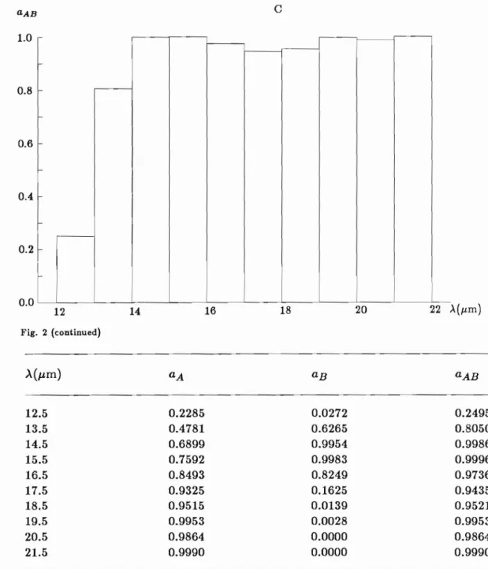
Fig. 2. Oomputed normal atmospheric absorptivity as a fundion of wave length, with l¡<m resolution. For H 20 (part Al, 00 2

at the (part

Bl

and H20 + 00 2 (part O).

1.0

0.8

0.6

0.4

0.2

0.0

e

1.0

0.8

0.6

0.4

aA an

we assun spectrurr for A

< ]

1982) th spectral

The rl

H20,

ce

values ca shown in

Figun and H2 (

microme

TABLE I. aA, aB and aAB are the present c1imate absoptivities due to H:¡O, CO:¡ and H:¡O + CO:¡, respective\y, corresponding to the wave length >'(¡lm) at intervals oC one micrometer.

The validity intervals of Smith's (1969) formulas are (12.5, 50J.lm) for H20 and (12.2, 19.8J.lm) for

C02. We will compute the absorptivity from A = 12J.lm on. In order to complete a one-micrometer step in the cases when there is a gap in the interval, we assume that the absorptivity is equal to zero in such gap; e.g., for the step (12, 13J.lm), we use aB = O in (12, 12.2J.lm ).

Once evaluated aA(A) and aB(A) for each one-micrometer step, we compute the combined absorp­

Fig. 3. A

ponding

m)

for >meter

;0 zero

bsorp-INTERAOTIVE LONG WAVE SPEOTRUM FOR THE THERMODYNAMIC MODEL 167

aA and aB are computed in the intervals (12, 50¡.tm) and (12, 20¡.tm), respectively. For A

>

20¡.tm we assume aB

=

O. Furthermore, from (1) we obtain aA

=

1 for A

>

22¡.tm. Therefore the combined spectrum is also saturated in the same region. Formula (1) and expression (2) are not applicable for A

<

12¡.tm. For this reason, we assume as in previous papers (Adem, 1962; Adem and Garduño, 1982) that for 8

<

A

<

12¡.tm, aAB = O; and that for A

<

8¡.tm, aAB = 1. Therefore the relevant spectral results discussed in this paper are in the interval (12, 22¡.tm).

The results of the computations are shown in Table 1 where the computed absorptivities due to H20, C02 and H20

+

C02 are shown in the second, third and fourth columns respectively. The values correspond to the wave length at intervals of one micrometer identified by their central values, shown in the first column.

Figure 2 shows the values of Table 1. Parts A, B and C are the absorptivities due to H20, C02 and H20

+

C02, respectively. In the three parts of the figure the abscissa is the wave length in micrometers and the ordinate is the absorptivity.

d) Comparation with other spectra

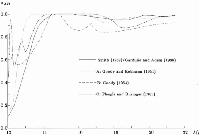
We looked for normal atmospheric spectra reported by other authors in order to compare them with that of Fig. 2C.

After a wide search we found only three different spectra:

A: The one computed by Goody and Robinson (1951).

B: The one, by Goody (1954).

C: The one given by Fleagle and Businger (1963).

1 . 0 / = - - - = . . : . . : =...

, I \ ., :"./"".: .

...~. ~

/

/ \ \ /"

' / " , - ' / \

----.--.-::"-

-

---- ­

/

-_...

"'-

-­

/

_/

/

/

/

I

l\ / /

, , !

\¡ /

0.6 \\ '.•' / _{- - - Smitb (1969)/Garduño and Adem (1988)}

i

V,-,/

A: Goody and Robinson (1951)

- - - - -B: Goody (1954)

0.4

- ' - ' - 0 : Fleagle and BUBinger (1963)

0.2

O . O ' - - - - L - - - - ' - - - ' - - - ' - - - ' - - - ' - - - ' - - - ' - - - ' - - - '

12 14 16 18 20 22 A(¡¡.m)

The spectrum Bis reproduced by Goody and Walker (1972). Fleagle and Businger (1963) report _{for H 20} the spectrum

e

without a clear information about its origino They mention the work of Goody and _The

_Sr

Robinson (1951), but spectra A and

e

are not the same. Kondratyev (1969) reproduces the spectrum _{(upper h}

A, attributing it to Goody (1954) instead of Goody and Robinson (1951). Houghton (1977) has an

(Peixóto

illustration of spectrum B without explaining its source. _hatched,

The spectra A, B and

e

are shown in Fig. 3, together with the spectrum of Fig. 2C, which is and T _{A :}

plotted as a curve instead of a histogram, in the interval from 12 to 21¡.tm. This figure shows that

Simila anyone of the four spectra does not coincide with any other anywhere, except between 14.5 and 15¡.tm,

duplicat€ where aH of them are saturated. We can see also that our spectrum is in very good agreement with

which ar, the spectrum A for A ::::: 15¡.tm, and in good agreement with the spectrum

e

between 13 and 14.5¡.tm,

cases we and again with spectrum A between 12 and 12.5¡.tm.

The spec Spectrum A is lower than ours from 15¡.tm on, probably because Goody and Robinson (1951)

computed it with an amount of 2 cm of water in the atmosphere, instead of the value 2.4 cm used by uso For A ::::: 15¡.tm _{the main absorber is H20 as can be seen in Fig. 2, and by reducing the H20}

content the spectrum is lowered as will be illustrated beHow. Goody and Robinson (1951) do not give data about the amount of CO 2 used in calculating the spectrum A.

The information given by Goody and Walker (1972), and by Fleagle and Businger (1963) about the spectra B and

e,

respectively, is not enough to explain discrepancies.

e) Spectra sensitivity

Now we illustrate the sensitivity of our spectra with respect to the gases (H20 and C02) content in the atmosphere. In order to show also the improvement obtained with an increment in the wave length resolution, we compute these spectra with steps of O.5¡.tm. These are plotted in Figs. 4 and 5

aA

Fig. 5. 001 261 cm ( O.314pm

Beside (with IJ.ll

results 01 00₂ con1

Comp~

(1969) fo more det wings, W

this is th new spec

12 14 16 18 20 22 ,\ (¡.¡m)

Fig. 4. Computed speetra íor H 2 0, with O.5¡.¡m resolution. The upper histogram corresponds to 2.50 cm, and the lower one to 2.25 1961). T cm oí H20. The hatched area indicates the difference between both cases.

1.0

0.8

0.6

0.4

0.2

0.0

F"""'" =

=~

=

~ ~

•

~

=

169

INTERAOTIVE LONG WAVE SPEOTRUM FOR THE THERMODYNAMIC MODEL

port and ;rum

LS an

eh is that

5/lm,

with

5/lm,

L951) used H₂0 o not

Lbout

mtent wave and 5

I to 2.25

for H 20 (Le., the graph of aA against >.) _{and for CO2 (Le.,} aB vs

>'),

respectively.

The spectra of Fig. 4 correspond to two cases: the absorptivity due to 2.5 cm of precipitable water (upper histogram) and for 2.25 cm (lower one). The value of UA = 2.5 cm is the actual average (Peixóto and Oort, 1984), thus we illustrate the effect of diminishing the H 20 content by 10%. The hatched area is the respective spectrum decremento Both cases are computed with P A

=

816.28 mb and TA

=

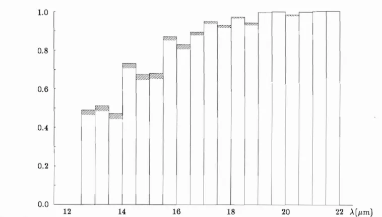
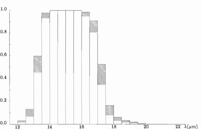
275.55 K, which are the values determined in subsection 6c.

Similarly, Fig. 5 shows the spectrum of C02 for its actual content (lower histogram) and for the duplicated one (upper histogram). The values of these contents were taken as UB

=

261 and 522 cm, which are the same ones used by us in previous papers (Adem and Garduño, 1982, 1984). In both cases we used the values PB

=

660.15 mb and T_B

=

263.43 K, which were determined in Seco 3. The spectral increment due to the doubling of CO 2, which is the hatched area, il3 equal to 0.374j.Lm.

1.0

0.8

0.6

0.4

0.2

0.0

14 16 20 22 A(jLm)

Fig. 5. Oomputed spectra for 002, with O.Sl'm resolution, using Smith's (1969) approach. The lower histogram corresponds to 261 cm of 002 , and the upper one to 522 cm. The hatched area, which indica tes the difference between both cases, is equal to O.374I'm.

Besides the spectra of Fig. 5 (with 0.5j.Lm resolution), we show in Fig. 6 the corresponding spectra (with 1j.Lm resolution) which were computed previously by us (Adem and Garduño, 1982), using the results of Yamamoto and Sasamori (1958, 1961). The spectral increment due to the increase of the C02 content from 261 to 522 cm, which is the hatched area, is in this case equal to O.303j.Lm.

.

,

1.0

0.8

0.6

0.4

0.2

12

-14 16 18 20

Fig. 6. Computed speetra for C02, with l.O,.m resolution, using Yamamoto and Sasamori's (1958, 1961) approach. The hatched area, which indicates the difference between both cases, is equal to O.303,.m.

Although its comparison with another one is not illustrated, the speetrum of H 20 has similar advantages than that of C02.

7. Final reIIlarks and conclusions

An attempt has been made to develop a parameterization of an interaetive long wave speetrum due to the atmospheric contents of water vapor and carbon dioxide adequate for use in a thermodynamic elimate model.

The numerical computations show that the speetrum for present elimate is realistic and that it is also sensitive to changes in the H20 and CO 2 contents. Furthermore, the parameterization allows to express the speetrum in terms of the surface temperature, the horizontal extent of eloudiness, and the mid-tropospheric temperature, variables which are ineluded in the elimate thermodynamic model. Therefore we hope that such parameterization can be used in such a model to simulate in a more realistic way the elimate. Preliminary experiments (Garduño and Adem, 1987, 1988) have shown that this is possible. However more complete experiments, using this parameterization, to compute the effect of an increase of the atmospheric CO 2 content and a change in the solar constant, will be carried out. The parameterization will also be used to possibly improve the simulation of the

elimates from the last glaciation, 18,000 years ago, to present (Adem, 1988).

This speetral formulation should be extended for A

<

12J.Lm, which is a regio n of great thermal importance for elimate. Similady, it is necessary to have absorptivity formulas for other atmospheric components, mainly 03, although it would be essential in this case, to extend the elimate model to inelude at least a stratospheric layer.

Acknow

We are ir and num,

Adem, J.

Adem, J. Wea.l

Adem, J. Geof. J

Adem, J.,

the lasl

Adem, J. atmosp

Adem, J.,

CO2 • (

Cerni, T. applica

EIsasser, Meteorl

Fleagle, R 346 pp. Garduño,

anaHtic de 1986 Garduño,

solar co Ensena(

Goody,

R.

Goody, R. Quart.

Goody, R.

Holton, J.

pp.

Houghton,

pp.

Kondratye

Liou, K. N

latched

imilar

m due namlC

~t it is allows iiness, 'namic late in ) have Ion, to

~stant,

of the

hermal spheric odel to

INTERACTIVE LONG WAVE SPECTRUM FOR THE THERMODYNAMIC MODEL 171

Acknowledgelllents

We are indebted to Alejandro Aguilar Sierra for his assistance in the programming, laser grafication and numerical computations, and to Francisco Hernández Acevedo for his valuable discussions.

REFERENCES

Adem, J., 1962. On the theory of the general circulation of the atmosphere. Tellus, 14, 102-115. Adem, J., 1967. Parameterization of atmospheric humidity using cloudiness and temperature. Mon.

Wea. Rev., 95, 83-88.

Adem, J., 1982. Simulation of the annual cycle of c1imate with a thermodynamic numerical model. Ceof. Int., 21, 229-247.

Adem, J., 1988. Possible causes and numerical simulation ofthe Northern Hemisphere c1imate during the Iast degIaciation. Atm6sfera, 1, 17-38.

Adem, J. and R. Garduño, 1982. Preliminary experiments on the climatic effect of an increase oí the atmospheric CO2 using a thermodynamic model. Ceof. Int., 21, 309-324.

Adem, J. and R. Garduño, 1984. Sensitivity studies on the c1imatic effect of an increase of atmospheric CO2 • Ceof. Int., 23, 17-35.

Cerni, T. A. and T. R. Parish, 1984. A radiative model of a stable nocturnal boundary layer with application to the polar night. J. Clim. Appl. Meteorol., 23, 1563-1572.

EIsasser, W. M., 1940. An atmospheric radiation chart and its use. Supplement to Quart. J. Roy. Meteorol. Soc., 66, 41-56.

Fleagle, R. G. and J. A. Businger, 1963. An introduction to atmospheric physics. Academic Press. 346 pp.

Garduño, R. and J. Adem, 1987. Resultados preliminares del modelo termodinámico con absortividad analítica en el infrarrojo. Memoria de la Reunión Anual de la UGM, en Morelia, Mich., noviembre de 1986.

Garduño, R. and J. Adem, 1988. Sensibilidad del modelo termodinámico respecto a la constante solar con interacción radiativa del vapor de agua. Memoria de la Reunión Anual de la UGM en Ensenada, B. C. N., noviembre de 1987.

Goody, R. M., 1954. Physics of the stratosphere. Cambridge Univ. Press.

Goody, R. M. and G. D. Robinson, 1951. Radiation in the troposphere and lower stratosphere. Quart. J. Roy. Meteorol. Soc., 77, 151-187

Goody, R. M. and J. C. G. Walker, 1972. Atmospheres. Foundations of Earth Sci. Ser.

Holton, J. R., 1979. An introduction to dynamic meteorology. 2nd ed., Academic Press, N. Y., 391 pp.

Houghton, J. T., 1979. The physics of atmospheres. Cambridge University Press. London, G. B. 203 pp.

Kondratyev, K. Ya., 1969. Radiation in the atmosphere. Academic Press., 912 pp.

Liou, K. N., 1980. An introduction to atmospheric radiation. Academic Press. N. Y., 392 pp.

'

Atm6·fera ( Manabe, S. and R. T. Wetherald, 1967. Thermal equilibrium of the atmosphere with a given distri­

bution of relative humidity. J. Atmos. Sci.,24, 241-259.

Manabe, S. and R. T. Wetherald, 1975. The effects of doubling the CO₂ concentration on the climate of a general circulation model. J. Atmos. Sci., 32, 3-15.

Paltridge, G. W., 1974. Global cloud cover and earth surface temperature. J. Atmos. Sci., 31, 1571-1576.

Peixóto, J. P. and A. H. Oort, 1984. Physics of climate. Rev. Mod. Phys., 56, 365-428.

Petukhov, V. K., 1974. The long-period process of heat and moisture exchange in the presence of broken clouds. IZ1J. Acad. Sci. USSR, Atmos. Oceanic Phys., 10, 219-227.

Ramanathan, V., 1976. Radiative transfer within the Earth's troposphere and stratosphere: a sim­ plified radiative-convective model. J. Atmos. Sci., 33, 1330-1346.

Schlesinger, M. E., 1984. Climate model simulations of CO2-induced climatic change. Adv. Geophys.,

26, 141-235. Dos experi

oceánico y

Sellers, W. D., 1973. A new global climatic model. J. Appl. Meteorol., 12, 241-254. _{tropical er}

la inmovili

Sellers, W. D., 1976. A two-dimensional global climatic model. Mon. Wea. Rev., 104, 233-248. _{que surge} Sergin, V. Y. and S. Y. Sergin, 1976. Paper 1 in "The simulation of the glaciers-ocean-atmosphere

planetary system" (S. Y. Sergin, ed.) 5-51. Far East Sci. Cent. USSR, Acad. Sci., Vladivostok. (In Russ.)

Two numE

Smith, W. L., 1969. A polynomial representation of carbon dioxide and water vapor transmission. the other in latitude

E.S.S.A. Tech. Rep. N.E.S.C. 47. planet, a t

Yamamoto, G. and T. Sasamori, 1958. Calculation of the absorption of the 15J.l carbon dioxide bando Sci. Rept. Tohoku Univ., Fifth Ser. 10, No. 2.

1. Intr. Yamamoto, G. and T. Sasamori, 1961. Further studies on the absorption of the 15J.l carbon dioxide

bando Sci. Rept. Tohoku Univ., Fifth Ser. 12, No. 1. One of t

the Indi the frarr moveme if SimplE

phenom.

2. Mod

2.1 Mas¡