Robust Model Error Estimation for Nonlinear Systems in H Infinity Framework

Robust Model Error Estimation for Nonlinear

Systems in H-Infinity Framework

Swetha Amit1, Raol, J. R.2

1

Asst. Professor, Dept. of Telecommunication, Ramaiah Institute of Technology and Research Scholar, Jain University, Bangalore. 2

Prof. Emeritus, Ramaiah Institute of Technology, Bangalore.

Abstract: Conventionally invariant embedding approach is used for determination of model discrepancy or error in nonlinear dynamic systems. In this paper, a robust approach based on H-infinity (HI) theory is presented. It is combined with the invariant embedding (IE) and the algorithms for continuous time and discrete time systems are presented. These estimators are evaluated with examples of nonlinear systems implemented in MATLAB.

Keywords: Deterministic discrepancy, model error, H-Infinity, invariant embedding, robust estimator.

I. INTRODUCTION

Mathematical modelling and system identification play very significant role in analysis of non-linear dynamic systems. When accurate models are not available, the approximate models are used in tracking and data fusion applications, especially in usual Kalman filter algorithm [1], which however, cannot determine explicitly the deterministic discrepancy, also called as model error [2]. This model error can be accurately determined by using the approach of invariant embedding, in deterministic setting [2]. In fact, a known (deficient or linear) model is used in the state estimation procedure, and deterministic discrepancy of the model is determined, using the measurements in the model error estimation procedure [3-5], assuming the data are from a nonlinear system. Once, this model error time history is available, one can fit another model to it and estimate its parameters using regression method; then adding the previously used deficient model and the new additional model (from the regression analysis) would yield the accurate model of the underlying (nonlinear) dynamic system (which has generated the data in the first place) [6].

The main aim of the proposed work is to provide a link between estimation of model error by (two-point boundary value problem and) using invariant embedding method (TPBVP/IE) and HI norm to arrive at a robust estimator. The method of combined IE and

H (HI) is discussed for continuous- as well as discrete-time systems. In essence, the robust estimators based on the classical LS

criterion in HI setting are presented. The performance of these algorithms is illustrated with simulations carried out in MATLAB.

II. H-INFINITY FRAMEWORK

The H norm provides a measure of a worst-case system gain. For a stable SISO linear system with transfer function ( ), the H

norm is defined as [7]:

‖ ‖ = max | ( )| (1)

or, in the event that the maximum may not exist, it is defined as

‖ ‖ = | ( )| (2)

In (1), | ( )| is a factor by which the amplitude of a sinusoidal input with frequency is magnified by the system, and is seen that

the H norm is simply a measure of the largest factor or gain.

The H norm can be usefully interpreted in terms of the effect of G on the space of inputs with bounded L2 norms. Let ( ) be a

signal with Laplace-transform ( ) such that the L2 norm given by ( ) =∫ ( ) is bounded. Then the system output

̃( ) = ( ) ( ) has L2 norm which is bounded by ‖ ‖ ‖ ‖ because,

‖ ‖ = ∫ | ( ) ( )| (3)

= ∫ | ( )| | ( )| (4)

≤ | ( )|. ∫ | ( )|

=‖ ‖ ‖ ‖ (5)

Hence,

‖ ‖ ≥‖ ‖

Thus, the H norm can be characterised as,

‖ ‖ = ‖_{‖ ‖}‖ , ≠0 (7)

The H norm gives the maximum factor by which the system magnifies the L2 norm of any input. Therefore, ‖ ‖ is also called the

gain of the system. Let ( ) have the state-space representation

̇( ) = ( ) + ( ) (8)

( ) = ( ) + ( ) (9)

so that the system transfer function is given as

( ) = ( − ) + (10)

The H norm of an error system matrix is given as [7, 8]:

for continuous system: ‖ ̃‖ = ∫ ̃( ) (̃ ) =∫ ̃( ) ̃( ) (11)

for discrete system: ‖ ̃‖ =∑ ∫ ̃( ) ̃( ) = ∮ ∫ ̃( ) ̃( ) (12)

For ̂ the transfer function matrix from the system disturbances to the estimate error; and one has ̃= − as estimate error,

and = as input disturbance [8]. For an H norm criteria, the transfer function (the peak energy gain), from the input

disturbances to the estimate error, ̂ , has a system gain with an upper bound

‖ _̂ ‖ < (13)

The performance bound criterion can also be written as

ǁ ̂ǁ

[ǁ ǁ ]< (14)

This criteria represents a family of solutions where the peak gain of the transfer function from the input disturbances to the estimate error is less than an upper bound . Hence, the performance criteria can be rewritten as:

(ǁ − ̂ǁ )− < 0 (15)

First the approach of IE is briefly discussed, then HI setting is combined with IE and the new robust estimators are presented.

III. INVARIANT EMBEDDING METHOD

In invariant embedding approach the particular solution that is sought is embedded in a general class and once this general case is solved, the particular solution can be obtained by using the special conditions, which have been kept invariant, in final analysis. Let the resultant equations from the TPBVP be given as [1, 6]

̇= ( ( ), (( ), ) (16)

̇_{=ψ( ( ), (( ), ) (17)}

The equations (16) and (17) represent the TPBVP with associated boundary conditions as: ( ) = and = . Now, though

the terminal condition = and time are fixed, one considers them as free variables. This makes the problem more general,

which includes the specific problem. It is known from the nature of the TPBVP that the terminal state depends on and

. Therefore, this dependency can be represented as

( ) = ( , ) = ( ( ), ) (18)

With → +∆ , one obtains by neglecting higher order terms

+∆ = + (̇ )∆ = +∆ (19)

One also gets, using (17) in (19)

+∆ = + ( , , )∆ (20)

and therefore,

∆ = ( , , ) ∆ (21)

Additionally, like (19), one obtains

+∆ = + ̇ ∆

and hence, using (16) in (22), one gets

+∆ , +∆ = , + , , ∆

= , + ( , , )∆ (23)

Using Taylor’s series:

+∆ , +∆ = , + ∆ + ∆ (24)

Comparing (23) and (24):

∆ + ∆ = ( , , )∆ (25)

or, using (21) in (25):

∆ + , , ∆ = ( , , )∆ (26)

Equation (26) simplifies to

+ , , ∆ = ( , , ) (27)

It is seen that (27) links the variation of the terminal condition ( ) = ( , ) to the state and co-state differential functions, (16)

and (17), and now in order to find an optimal estimate ( ), one needs to determine ( , ) as

= ( , ) (28)

Equation (27) can be transformed to an initial value problem by using approximation

, = + ( ) (29)

Substituting (29) in (27):

( )

+ ( )+ ( ) , , = ( , , ) (30)

Next, expanding and about , , and , , to obtain

, , = , , + , , , −

= , , + , , (31)

and

, , = , , + , , (32)

After considerable algebraic development, avoided here for brevity [1, 6], one finally obtains the following composite IE based estimator:

( )

( ) +

( )

+ [ , , + , , ] = , , + , , ( ) (33)

In (33), c = , and equation (33) can be separated by substituting the specific expressions for in (33); and this is done

after specifying the dynamic systems for which one needs to obtain the estimators. This is done for the robust algorithms next.

IV. ROBUST CONTINUOUS TIME ALGORITHM

The general optimal control problem concerns the minimization of some function (functional) J, the performance index (or cost functional). Let the mathematical description of dynamic system be given as

̇= ( ( ), ( ), ) + ( ) (34)

( ) = ( ) + ( ) (35)

The basic cost function is given by [9]

=∫ ( )− ( ) ( )− ( ) + ( ( ) ( )) (36)

In (36), ( ) is the model discrepancy/error to be determined simultaneously with ( ), ( ) is the spectral density matrix of noise

and ( ) is the spectral density matrix of the deterministic discrepancy. In [9], more generalized IE estimators at alpha level were

presented and evaluated. Here, the similar approach is used, however, the estimators are extended to HI frame work. The cost function for the combined approach, the classical least squares (LS) and the HI based is formulated as

= || − ̂|| − || || (37)

=∫ ( )− ( ) ( )− ( ) − ( ( ) ( )) (38)

Let the mathematical description of dynamic system be given as

̇= ( ( ), ) + ( ) (39)

( ) = ( ) + ( ) (40)

In (39), ( )is the state vector, and the control input is dropped, and ( ) is the measurement vector with noise ( ). The

un-modelled part of the model is represented by ( ), which is assumed to be piecewise continuous, and is termed as deterministic

discrepancy, or model error. The term ( ) can be determined using an optimization method by minimizing the cost function J:

=∫ ( )− ( ) ( )− ( ) − ( ( ) ( )) (41)

In (41), the second term is influenced by the H-infinity framework, and that would yield a robust model error estimator. The Lagrange multiplier is used to incorporate the constraint of the system dynamics (39), and the modified cost function is obtained as

=∫ ( )− ( ) ( )− ( ) − ( ( ) ( )) + ( ̇( )− ( ( ), )− ( )) (42)

From (42), the Hamiltonian is defined as

= ( ( )− ( )) ( )− ( ) − ( ) ( )− [( ( ( ), ) + ( )] (43)

= − ( ( ), ( ), )

In (43) one has

= ( )– ( ) ( )– ( ) − ( ) ( ) (44)

By straightforward development paralleling [1,9] (the details are avoided here), one obtains the following equations

= =− + (45)

̇_{= − =− −2 ( )− ( ) (46)}

and

= 0 =− + (47)

=− (48)

Thus, the TPBVP is

̇= ( ( ), ) + ( ) (49)

̇_{= −2} ( )− ( ) − (50)

=− (51)

( ( ), ( ), ) = ( ( ), ) + ( ) (52)

( ( ), ( ), ) =−2 ( )− ( ) − (53)

and,

= = 2 − ( ) (54)

= (55)

The TPBVP results in the composite equation similar to (33); with associated boundary conditions as ( ) = and = . The

separation of the state estimator and the ‘covariance’ estimator results into

̇_{( ) = 2} ( ) ( )− ( ) + ( ( ), ) (56)

̇

( ) = ( ) −2 ( ) ( ) − + ( ) + ( ) ( )

(57)

Dividing (57) by and setting ⟹0, one obtains

̇_{( ) = ( )} −2 ( ) ( )− + ( ) (58)

One also gets an explicit expression for model error (discrepancy) as

( ) = 2 ( ) ( )− ( ) (59)

V. ROBUST DISCRETE TIME ALGORITHM Consider a nonlinear system given by

( + 1) = ( ( ), ) (60)

( ) =ℎ( ( ), ) (61)

Writing (60), (61) more explicitly with the model error, and measurement noise, one obtains

( + 1) = ( ( ), ) + ( ) (62)

( ) =ℎ( ( ), ) + ( ) (63)

The model error is estimated by minimizing the cost function criteria

= ∑ ( )− ℎ( ( ), ) ( )− ℎ( ( ), ) − ( ) ( ) (64)

Using the concept of Lagrange multiplier to handle the constraint within the function J, one obtains

= ∑ [ ( )− ℎ( ( ), ) ( )− ℎ( ( ), ) − ( ) ( )] + [ ( + 1)− ( ( ), )− ( )]

(65) The Euler-Lagrange conditions [1] along with robust scheme yield the final estimator equations as

( + 1) = ( ( ), ) + 2 ( + 1) ( + 1) [ ( + 1)− ℎ( ( + 1), + 1] (66)

( + 1) = [ + 2 ( + 1) ( + 1) ( + 1)] ( + 1) (67)

( + 1) = ( ( ), ) ( ) ( ( ), )− (68)

( ) = 2 ( ) ( ) [ ( )− ℎ( ( ), )] (69)

with ( ) = ( ( ), )_{( )}

( ) ( ) and

=− ( ) (70)

VI. EVALUATION OF THE ALGORITHMS

Considering the following nonlinear continuous time system [1]

̇ _{( ) = 2.5 cos( )−0.68 ( )− ( )−0.0195 ( ) (71)}

̇ _{( ) =} ( ) (72)

The model error is determined by eliminating the following terms from (71) in turn: (i) (t), (ii) , , , and utilizing the

deficient models in the corresponding estimation algorithm. Then, a regression model is fitted to the discrepancy ( ) = ( ) +

( ) + ( ) to estimate the parameters of the continuous-time nonlinear system. Values Q=diag(0.001, 30) and R=18 are

used for this example for achieving convergence. The term  is used that would generate a robust estimator in finding the states of

the system and the model error. The parameters are estimated from the model discrepancies using LS method. Table 1 shows the estimates of the coefficients compared with the true values for the two cases. The estimates compare well with the true values of the parameters. It is to be noted that in all the cases, from the estimated model discrepancy, the parameter that is removed from the model is estimated. Figure 1 shows the comparison of the simulated and estimated states and Figure 2 shows the comparison of the estimated model discrepancies compared with the true model error. The match is very good and it indicates that the model discrepancy is estimated accurately by the algorithm.

Next, considering a nonlinear discrete system [1]

( + 1) = 0.8 ( ) + 0.223 ( ) + 2.5 cos(0.3 ) + 0.8 sin(0.2 )−0.05 ( ) (73)

( + 1) = 0.5 ( ) + 0.1 cos(0.4 ) (74)

The model error is determined by eliminating the following terms from (73) in turn: (i) , (ii) , , and (iii) , , . To the

model error thus estimated, a regression model is fitted: ( ) = ( ) + ( ) + ( ) + ( ) to estimate the

parameters of the discrete nonlinear system. 100 samples of data are generated using (73) and (74). It is to be noted that although the

term containing is not present in the true model of the system, it is included to check the performance of the algorithm. Table 2

shows the parameters estimates compared with the true values for the three cases by introducing HI framework with suitable gamma values. The estimates compare very well with the true values of the parameters. It is to be noted that in all the cases, from the

estimated model discrepancy, the parameter that is removed from the model is estimated. In all the cases, the term is estimated

and estimated model states. Figure 4 shows the estimated model discrepancy d(k) compared with the true model discrepancies for all the cases. The good match indicates good estimation of the model discrepancy.

VII. CONCLUSION

New estimator algorithms based on the combined approach of invariant embedding and the robust H-infinity frame work for continuous time as well as discrete time nonlinear systems are presented. These algorithms also obtain the model errors in nonlinear systems. The performances of these estimators are evaluated using numerical simulations carried out in MATLAB. The results are found to be very encouraging.

REFERENCES

[1] Raol, J. R., Girija G., and J. Singh. Modelling and Parameter Estimation of Dynamic Systems. IET/IEE Control Series Books, Vol. 65, IET/IEE society, London,UK,2004.

[2] Datchmendy, D.M., and Sridhar, R. Sequential estimation of states and parameters in noisy nonlinear dynamical systems. Trans. of the ASME, Jl. of Basic Engineering, pp. 362-368, USA, June 1966.

[3] Mook, D. J., and Junkins, J. L. Minimum model error estimation for poorly modelled dynamic systems. AIAA 25th aerospace sciences meeting (AIAA-87-0173), Reno, Nevada, USA, 1987.

[4] Mook,D.J. Estimation and identification of nonlinear dynamic systems, AIAAJl., Vol.27, No.7, pp.968-974, USA, July1989.

[5] Crassidis, J. L, Markley, F. L., and Mook, D. J. A real time model error filter and state estimator, In Proc. of AIAA Conf. on Guidance, Navigation and Control, Arizona, USA, Paper No. AIAA-94-3550-CP, Aug. 1-3, 1994.

[6] Parameswaran, V., and Raol, J. R. Estimation of model error for nonlinear system identification, IEE Proc. Control Theory and Applications, Vol. 141, No. 6, pp. 403-408, Nov., 1994.

[7] B. Hassibi, A.H. Sayed and T. Kailath.Linear estimation in Krein spaces - Part I: Theory, IEEE Trans. Automatic Control, Vol. 41, No. 1, pp. 18-33, Jan 1996. [8] Rawicz, P. L. HI/H2/Kalman Filtering of Linear Dynamical Systems via Variational Techniques with Applications to target tracking, Ph.D. thesis, Drexel

University, December 2000.

[9] Swetha, A., and Raol, J. R. Generalized model error estimators for nonlinear systems. International Journal of Enhanced Research in Science, Technology & Engineering (IJERSTE- ISSN: 2319-7463), Vol. 5 Issue 7, pp. 77- 89, July2016

.

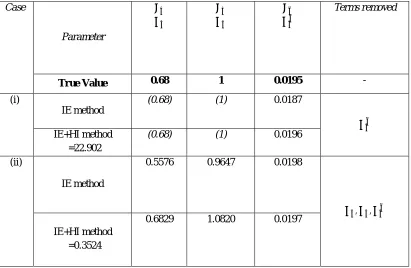
Table 1: Nonlinear parameter estimation results-CTS-case (i) and case (ii)

Case

Parameter

Terms removed

True Value 0.68 1 0.0195 -

(i)

IE method

(0.68) (1) 0.0187

IE+HI method

=22.902

(0.68) (1) 0.0196

(ii)

IE method

0.5576 0.9647 0.0198

, ,

IE+HI method

=0.3524

Figure 1: Time history match – states for case (i) and case(ii)

Figure 2: Time histories of model discrepancies d(k) case (i) and case(ii)

Table 2: Nonlinear parameter estimation results – Discrete-time system

Case Parameter Terms

removed

True values 0.8 0 -0.05 0.223 -

(i) IE method (0.8) -1.03e-5 -0.0498 (0.223)

IE+HI method = 0.5

(0.8) -0.0000 -0.05 (0.223)

(ii) IE method 0.7961 -8.3e-6 -0.0498 (0.223)

, IE+HI method

= 7.5

0.8 -0.00 -0.0499 (0.223)

(iii) IE method 0.8000 -3.07e-7 -0.05 0.2224

, ,

IE+HI method = 0.2

Figure 3: Time history match-states X1 and X2