Analysis of Heat Exchanger Process with Long Dead Time

Analysis of Heat Exchanger Process with Long

Dead Time

Shanu Khan

#

Electronic Instrumentation & Control Department, Global College of Technology Jaipur

Abstract- This paper presents the analysis of time delayed system controlled by a Proportional Integral controller and smith predictor to compensate the long dead time occurred in a process. For a test bed purpose a heat exchanger model is used. In order to generate modelling of shell and tube heat exchanger a Levenberg marquardt algorithm is used which trains artificial neural network 10 to 100 times faster than the usual back propagation algorithm. The generated first order plus dead model show the delayed time of -23.6 sec. Smith predictor is used to adjust the settling time more quickly as compare to Proportional integral controller and compensate the process. The generated result shows more effectiveness as compared to the previous result using MATLAB simulation software. Frequency analysis for the robustness is performed.

Keywords- Artificial neural network, proportional Integral controller, Levenberg marquardt algorithm, Shell and tube heat exchanger, Smith predictor

I. INTRODUCTION

Systems with delays can be usually encountered in the real world. When the system involves propagation and transmission of information or material, the delay is certain to occur. The presence of delays complicates the system analysis and the control design. Such process may be called as dead time process. For processes with long time delays it is often difficult to achieve good control using just PID control strategies. Such application may handled by smith predictor. Dead times appear in many processes in industry and in other fields, including economical and biological system. They are caused by some of the following phenomena like the required processing time for sensors; such controllers need some time to implement a complicated control algorithm or process. The non linear system like heat process model is affected by the uncertainties and cannot be modeled easily. The process may exhibits time delay in the system which need to be control for closed loop specification. This paper presents the modeling of heat exchanger using Levenberg marquardt algorithm which trains artificial neural network 10-100 times faster than the usual back propagation is a steepest decent algorithm [3]. After modeling of shell and tube heat exchanger a First order plus dead time

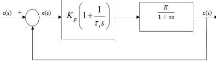
[image:2.612.331.554.500.570.2]

(FOPDT) model is generate by using two point and three point system identification processes [4]. A smith predictor is designed to control the long dead time process. PI controller is limited to high overshoot and large settling time as compared to the more effective Smith Predictor control strategy. Simulation results show capabilities of the system as well as the disturbance rejection.Figure 1 shows the simple PI controller structure.

Fig 1. Simple PI Controller

The transfer function of PI controller is given by

















2

1

( ) 1

1

( ) 1

1 1

i i

p i i p i p

i i

s s

e s

KK s

r s s KK s KK

s s

 

  

 



 

    

( ) = ( )

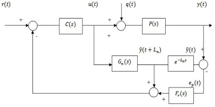
[image:3.612.46.260.201.308.2]

Where G(s) is a delay free transfer function and is the time delay.

Fig 2: Structure of Filtered Smith Predictor (FSP)

In figure 2, the filter should be designed to attenuate oscillations in the plant output especially at the frequency where the uncertainty errors are important and it is given by



0.202 *1 1



F

s





Here F is used as a filter to remove dead time estimation

II. MODELING OF HEAT EXCHANGER

The Mathematical model of Shell and Tube Heat Exchanger is developed by using Levenberg Marquardt Algorithm. This algorithm train’sartificial neural network 10 to 100 times faster than the usual back propagation algorithm is the Levenberg-Marquardt algorithm. While back propagation is a steepest descent algorithm, the Levenberg-Marquardt algorithm is a variation of Newton's method.

 

₂

 

1

 

 

 x   _ V x _ V x

 

 

2

 

1







N _i  _i

i

S x e x e x

 

   

2

  T

V x J x J x

              2 1 2 1 2 1 2  _{  }              _{  }     _{  }         n

N N N

n

e x

e x e x

J x x x x

e x e x e x

x x x

   

1

   

 

   x JT x J x  JT x e x

   

1

   

 

  _ T  _ T

x J x J x I J x e x

   





2

1   



M m

y m d m

M S E

M













2

2

2 1 1

2 1 ˆ        







M M

m m m

m m

M i m

y y y y

R y y





 





2 2 1 1 2 1 ˆ        







M M

m m m

m m

M i m

y y y y

R

y y

Where,

y

_m = the observed dependent variable

ˆ

_m

y

= the fitted dependent variable for the independent variable

m

x

y

= mean,

y

_m

y

m

M





x

_m= the independent variable in the

th

m

trial





2 1 M m m

y

y







r e p r e s e n t s t o t a l s u m o f s q u a r e s , w h i l e





2

1

ˆ

M m m m

y

y





[image:4.612.35.273.110.293.2]

Fig 3. Instrumentation diagram of Shell and Tube Heat Exchanger

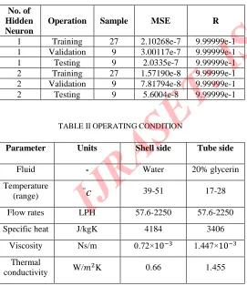
TABLE I PERFORMANCE EVALUATION OF TRAINING, VALIDATION AND TESTING

No. of Hidden Neuron

Operation Sample MSE R

[image:4.612.341.549.150.300.2]

1 Training 27 2.10268e-7 9.99999e-1 1 Validation 9 3.00117e-7 9.99999e-1 1 Testing 9 2.0335e-7 9.99999e-1 2 Training 27 1.57190e-8 9.99999e-1 2 Validation 9 7.81794e-8 9.99999e-1 2 Testing 9 5.6004e-8 9.99999e-1

TABLE II OPERATING CONDITION

Parameter Units Shell side Tube side

Fluid - Water 20% glycerin Temperature

(range)

c

 _{39-51 17-28}

Flow rates LPH 57.6-2250 57.6-2250 Specific heat J/kgK 4184 3406

Viscosity Ns/m 0.72×10 1.447×10 Thermal

conductivity W/ K 0.66 1.455

Fig. 4: Regression plots for actual and predicted results by feed-forward neural network model for training, validation, testing

samples and all data set

[image:4.612.20.291.370.684.2]

R Square is a measure of the explanatory power of the model. Here for best model chosen R Square is1, for training, 1 for validation and 1 for testing respectively as shown in figure 4. In figure 4 the dashed line is the perfect fit line where outputs and targets are equal to each other. From the graph 5, it can be realized that the best hidden unit with 99% accuracy is with just one neuron with one trial for this model.

[image:4.612.337.552.451.614.2]

neurons. The training stops when MSE do not change significantly.

First the FOPDT Model is given by

( ) 1

p s

K

P s e

s     

And for shell and tube heat exchanger model it is given by

 

23.6

12.56 1 s p e G s s   

There are many admissible transfer functions for the same process defined by each possible combination of, K_pand.

Here for study of this process two representative plant models considered i.e.

 

 

24.2 2 3 1 .2 1 1 .5 6 1

0 .4 1 3 .5 6 1

s p s p e G s s e G s s      

T h e s te p r e s p o n s e o f th e F O P D T w ith lo n g d e a d tim e is g iv e n in fig u r e 1 . H e r e th e d e la y p r o v id e d in th e s y s te m is 2 3 .6 s e c

F ig 6 . S te p r e s p o n s e o f F O P D T M o d e l

F ig 7 .W ith I n c r e a s in g G a in

N o w d if fe r e n t v a lu e s o f K_p i.e . 3 , 0 .2 7 a n d 0 .4 a r e u s e d a n d

v a r ia tio n in s te p r e s p o n s e is s h o w n in F ig u r e 7 . F r o m F ig u r e 7 , it is c le a r th a t in c r e a s in g th e p r o p o r tio n a l g a in K_p s p e e d s u p th e

r e s p o n s e b u t a ls o s ig n ific a n tly in c r e a s e s o v e r s h o o t a n d le a d s to in s ta b ility . T h is s y s te m h a s a lo n g d e a d tim e . N o w w h e n a P r o p o r tio n a l in te g r a l c o n tr o lle r is a p p lie d o n th is s y s te m w ith

0 .2 7 8 1

p

K  a n dTi 1 0 .2 , th e r e s u lt o b ta in e d is s h o w n in

F ig u r e 8 .

F ig 8 . S te p r e s p o n s e w ith Kp 0 .2 7 8 1 a n d Ti 1 0 .2

0 20 40 60 80 100 120

0 0.1 0.2 0.3 0.4 0.5 0.6 0.7 0.8 0.9 1

From: u To: y

Step Response

Time (sec)

Time (sec)

0 20 40 60 80 100 120

0 0.5 1 1.5 2 2.5

0 100 200 300

-0.2 0 0.2 0.4 0.6 0.8 1 1.2 1.4 From: ysp

0 100 200 300

From: d

Step Response

[image:5.612.349.543.471.641.2]

[image:6.612.311.544.163.567.2]

From Figure 9, it is clear that Smith Predictor provides much faster response as compared to proportional Integral controller and here also Smith Predictor rejects the disturbance earlier as compared to Proportional integral controller. Moreover the settling time and various parameters are given in table III.

Fig 9. Step response, PI v/s Smith Predictor

The Smith Predictor provides much faster response with no overshoot as clearly shown in the result obtained. Here the result getting from smith predictor much improved then the PI controller

TABLE III COMPARISON OF DIFFERENT PARAMETERS IN CONTROLLERS

S.

No. Parameters PI Controller Smith Predictor

1 Settling Time 196 Sec. 36.5 Sec. 2 Rise Time 32.8 Sec. 8.59 Sec.

3 Peak

Amplitude 1.19 1.02

4 Overshoot 18.7% 1.64%

The difference is also see in the frequency domain by plotting the closed-loop Bode response from Y_sp to Y . Note the higher

bandwidth for the Smith Predictor. Figure 10 show the closed loop Bode- plot of given transfer functions. Also smith

predictor controller rejects the disturbance earlier as compared to PI controller. Overshoot and settling time are less as compared to PI controller.

Fig 10. Bode Plot of PI v/s Smith Predictor

Fig 11. Step respone of PI v/s Smith Predictor

CONCLUSION

In this paper modeling and analysis of shell and tube heat exchanger process is done using Levenberg marquardt algorithm. When compared to the classical proportional controller, the Smith Predictor greatly improves the systems response to set-point changes as given in table III.

0 100 200 300

-0.2 0 0.2 0.4 0.6 0.8 1 1.2 1.4

From: ysp

0 100 200 300

From: d

Step Response

Time (sec)

Smith Predictor PI Controller

-40 -30 -20 -10 0 10

From: ysp To: y

10-3 10-2 10-1 100

-1800 -1440 -1080 -720 -360 0

Bode Diagram

Frequency (rad/sec)

Smith Predictor PI Controller

0 100 200 300

From: d

Step Response

Time (sec)

0 100 200 300

-0.4 -0.2 0 0.2 0.4 0.6 0.8 1 1.2 1.4

[image:6.612.343.543.378.551.2]

[1] Hagan and Menhaj, 1994: Training feed forward networks with the Marquardt algorithm. IEEE Trans. on Neural Networks, 5(6), pp. 989993.

[2] Pandharipande S L, Siddiqui M A, Dubay A & Mandavgane S A, Indian Journal of Chemical Technology, Volume 13, November 2006, pp. 634-639

[3] M.R. Matausek and A.D. Micic. “A Modified Smith Predictor for Controlling a Process with an integrator and Long

Dead Time” IEEE transactions on automatic control, Vol.41, No.8, pp.1199-1203, August 1996.

[4] G.Saravanakumar, R.S.D.WahidhaBanu, V.I.George” Robustness and Performance of Modified Smith Predictors for Processes with Longer Dead-times” ACSE Journal, Vol. 6, Issue (3), pp.41-46,Oct.,2006.

[5] Hossam A. Abdel Fattab, Ahmed M. Gesraba and Adel A.

Hanafy “Control of Integrating Dead Time Processes with Long

Time Delay” American Control Conference Boston,

Massachurelts, pp.4964-4970, June 30-July 2, 2004

[6] G. Alevisakis and D. Seborg “An Extension of the Smith predictor to Multivariable Linear Systems Containing Time