Enhancement to TV Greedy Algorithm to Minimize Sensor Movement for Target Coverage and Network Connectivity in Mobile Sensor Networks

Enhancement to TV-Greedy Algorithm to

Minimize Sensor Movement for Target Coverage

and Network Connectivity in Mobile Sensor

Networks

Pallawi M.Bhandurge1, S.A. Hashmi2 1

M. Tech Scholar (Computer Networks and Internet Security), Department of Information Technology, MGM’s College of Engineering, Nanded (M.H.), India

2

Asst. Professor & Head, Department of Information Technology, MGM’s College of Engineering, Nanded (M.H.), India

Abstract: Coverage of interest points and network connectivity are two main challenging and practically important issues of Wireless Sensor Networks (WSNs). Although many studies have exploited the mobility of sensors to improve the quality of coverage and connectivity, little attention has been paid to the minimization of sensors’ movement, which often consumes the majority of the limited energy of sensors and thus shortens the network lifetime significantly. To fill in this gap, this work addresses the challenges of the Mobile Sensor Deployment (MSD) problem and investigates how to deploy mobile sensors with minimum movement to form a WSN that provides both target coverage and network connectivity. To this end, the MSD problem is decomposed into two sub problems: the Target Coverage (TCOV) problem and the Network Connectivity (NCON) problem. We then solve TCOV and NCON one by one and combine their solutions to address the MSD problem. To solve TCOV problem, the TV-Greedy algorithm based on Voronoi partition of the deployment region, is proposed to reduce the total movement distance of sensors. For NCON, an efficient solution based on the Steiner minimum tree with constrained edge length is proposed. The enhancement to TV-Greedy algorithm is proposed which further optimizes the solution when targets are in close proximity to each other. The combination of the solutions to TCOV and NCON, as demonstrated by extensive simulation experiments and performance measures, offers a promising solution to the original MSD problem that balances the load of different sensors and prolongs the network lifetime consequently.

Keywords: Wireless sensor networks, target coverage, network connectivity, mobile sensors, TV-Greedy

I. INTRODUCTION

Wireless Sensor Network (WSNs) is a new emerging application of ad-hoc networks which provide high monitoring quality for massive geographical areas with relatively inexpensive equipment. Wireless Sensor Networks (WSNs) are currently used in a wide range of applications including environmental monitoring and object tracking to improve system performance, provide convenient and efficient method and can also fulfil functional requirement. Ensuring coverage and connectivity is a fundamental objective of wireless sensor network. The coverage of sensor network represents the quality of supervision that the network can provide, that is how well the region of interest is being monitored by sensors, and how effectively a sensor network can detect intruders [2]. In many applications, sensors are not mobile and remain stationary after their initial deployment.

The coverage of such a stationary sensor network is determined by the initial network configuration. Once the deployment strategy and sensing properties of the sensors are known, then the network coverage can be calculated and remains unchanged over time. Similarly connectivity is also necessary for sensor in WSN to collect data and report data to the sink node.

II. PROPOSEDSYSTEM A. System definition

Sensor movement is major factor that affects network lifetime since, it often consumes majority of the limited energy supply of sensors. This dissertation topic mainly focuses on minimization of sensors’ movement to provide target coverage and network connectivity. For this, the Mobile Sensor Deployment (MSD) problem is defined to deploy mobile sensors to provide target coverage and network connectivity at minimum movement cost [1]. The formal definition of the MSD problem is as below.

B. Mobile Sensor Deployment (MSD) problem

Given m targets with known locations and n mobile sensors deployed randomly in the task area, the MSD problem seeks the

minimum movement of mobile sensors such that the following objectives are achieved after mobile sensors reach their new positions:

The MSD problem concerns two issues, namely target coverage and network connectivity. Hence it is further divided into two sub problems and solved independently. First, mobile sensors are deployed to cover targets with minimum movement. These mobile sensors are called coverage sensors. Then, the rest sensors are deployed to provide connectivity between coverage sensors and the sink. The definitions of the two sub-problems are given below.

1) Target Coverage (TCOV) problem: Given m targets with known locations and n mobile sensors deployed randomly in

the task area, How to determine the sensors to be deployed and their new positions such that all the targets are covered and the total cost of movement of sensors is minimum.

2) Network Connectivity (NCON) problem: Given a sink that collects data sensed from targets by sensors, the set of

coverage sensors determined by TCOV and the remaining mobile sensors in task area, How to determine the remaining sensors to be deployed and their new positions such that coverage sensors and the sink are connected and the total cost of movement of sensors is minimum.

C. System Model

In the system model addressed in this study, there are m targets T = {t1 ,. . . , tm} with known locations to be covered and n mobile

sensors S = {s1 ,. . . , sm} randomly deployed in the task area. The system model works as follows:

1) Every mobile sensor knows its own position via a mounted GPS unit or a localization service in the network. We also assume

that, there is a control center, e.g., a sink, which collects sensors’ location information and broadcasts movement orders to mobile sensors.

2) The task area is free of obstacles against movement. For the case with obstacles, a sensor is able to choose an appropriate

shortest path to the destination to bypass the obstacles on the way. In this work, we focus on determining which sensors should move and WHERE they should move to in order to guarantee both target coverage and network connectivity.

3) Network model. Disk model [3] is adopted for both sensing and communication of sensors with the sensing radius rs and the

communication radius rc, respectively. Each target can be covered by more than one sensor, and each sensor can cover more

than one target. A target is said covered if and only if there is at least one sensor in the disk of radius rs centered at the target.

The disk is defined as the target’s coverage disk, and the circle of the coverage disk is called the target’s coverage circle.

4) Mobility model. The free mobility model [4] is adopted. In this model, sensors are able to move continuously in any direction

and stop anywhere. The distance that a sensor moves is used to present the sensor’s energy consumption incurred in the

movement. The movement distance of sensor s to cover target t is dist(s, t) - rs, where dist(s, t) is the Euclidean distance

between s and t. Similarly, the movement distance of sensor si to connect with sensor sj is dist(si, sj) – rc, where dist(si, sj) is the

distance between si and sj. In the obstacle-free scenario, in order to minimize the movement distance of a sensor to a target, the

sensor should move along the straight line from its initial position to the target until it reaches the target’s coverage circle.

III. SOLUTIONTOTCOVANDNCON

The two main sub problems - Target Coverage and Network Connectivity are solved independently one by one and then solutions to them are combined to get solution to whole MSD problem.

A. Solution to Target Coverage(TCOV) problem

Voronoi based TV-Greedy algorithm is that it accurately identifies the sensors that can cover a target based on Voronoi diagram of targets, thereby reducing the coverage cost of targets.

Before, going into details of the TV-Greedy algorithm, the key terms related to it are explained as below.

1) Voronoi Diagram: Voronoi diagram is the partitioning of a plane with points into convex polygons such that each

polygon contains exactly one generating point and every point in a given polygon is closer to its generating point than to any other [5]. It is created by taking pair of points close to each other and drawing a line between them which is equidistant to the two points and perpendicular to the line connecting the two points [6]. All the points on the lines in diagram are equidistant to the two generating source points.

Fig.1. Voronoi diagram

2) Own Server Group (OSG): If a sensor is located inside a target’s Voronoi polygon, the sensor is said to be Server to that

target, and the target is regarded as Client of its servers. The group of target’s servers is called as Own Server Group (OSG) of target.

That is the sensors that are present in the target’s voronoi polygon form the Own Server Group of the target.In Fig. 2, the blue filled

circles represent the Own Server Group of the given target marked as red filled triangle. The sensors which are present in the target’s voronoi polygon forms the OSG of the target.

Fig.2. Own server group

3) Chief Server: Out of the servers in target’s OSG, the sensor which is closest to the target is called the Chief Server of that

target.In Fig 3, red filled circle represents the chief server of the given target marked as red filled triangle.

4) Candidate Server Group (CSG): Two targets are neighbors, if their Voronoi polygons share an edge [6]. The sensor in a target’s OSG that is closest to its neighbor target is called as an Aid Server for that neighbor target. A target’s candidate server

group (CSG) is the union of its own Chief Server and all the Aid Servers from neighbors.In Fig 4, the green filled circles represent

the CSG of the given target marked as red filled triangle. Only the server from CSG of a target will be dispatched to cover it.

Fig.4. Candidate server group

5) TV-Greedy Algorithm:

Input: T = t1 , t2 , . . . , tm ;//The position of all targets

S = s1 , s2 , . . . , sn ;//The position of sensors

rs ;//The coverage radius

Output: tmc; //The total movement cost

Step 1 Generate the Voronoi diagram (VD) of targets.

Step 2 Using Voronoi polygon, determine neighbors for each target.

Step 3 Determine the OSG for each target using S and VD.

Step 4 For each OSGi do Steps 5 and 6.

Step 5 Determine the Chief Server for Target ti.

Step 6 Identify the Aid Servers for ti ‘s neighbor targets.

Step 7 For each Target ti do Steps 8 to 13.

Step 8 Check if ti is already covered. If yes then set cost(ti) = 0 and go to Step 13. Else go to Step 9.

Step 9 Produce CSGi of target ti. If CSGi is not Empty then go to Step 10. Else go to Step 11.

Step 10 Move the nearest server from CSGi to cover target ti and set cost(ti) = movement distance and go to Step 13.

Step 11 If there exists neighbors’ chief servers that could be shared then move the nearest chief server to cover ti. Set cost(ti) =

movement distance and go to Step 13. Else go to Step 12.

Step 12 Regenerate the CSG of ti by searching aid servers of the ti’s 2nd or higher order neighbors and move the nearest aid server

to cover ti . Set cost(ti) = movement distance and go to Step 13.

Step 13 Set tmc = tmc + cost(ti).

Step 14 Return tmc

B. Solution to Network Connectivity (NCON)Problem

After the TCOV problem is solved, we get the coverage sensors for all the targets and their new location after movement to cover the targets. Next we need to solve problem of the connectivity of sensors and the sink, which is required for transmitting the sensed data to the sink. If the sink and the coverage sensors are already connected, then the connectivity problem is already solved. Otherwise, NCON problem need to be solved.

The basic idea of solving NCON problem is to relocate the rest mobile sensors to some locations where they can act as relay nodes and transfer data from coverage sensors to the sink.

The ECST-H algorithm solves NCON problem in two steps. First, it constructs an edge length constrained Steiner tree spanning all

the coverage sensors and the sink, such that each tree edge length is no longer than rc . The Steiner tree is required to minimize the

number of sensors that need to move. Second, it moves the rest mobile sensors to the generated Steiner points to connect the coverage sensors and the sink. The second step can be thought of as a special case of TCOV where the Steiner points are considered as “target”s and the coverage radius is taken as zero. Then we can apply TCOV to dispatch sensors to cover that “target” s. Following are the key terms related to the ECST algorithm.

1) Minimum Spanning Tree: It is a subset of the edges of a connected, edge length undirected graph that connects all the vertices together, without any cycles and with the minimum possible total edge length i.e., it is a spanning tree whose sum of edge

length is as small as possible [7].Fig 5 shows the minimum spanning tree for the vertices marked as red filled circles.

Fig.5. Minimum Spanning Tree

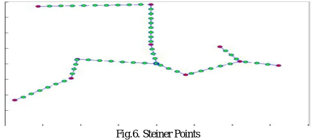
2) Steiner Points: They are the extra intermediate vertices added in minimum spanning tree in order to restrict the maximum

length of an edge in spanning tree.Fig 6 shows the Steiner points marked as green filled circles added to the edges of minimum

spanning tree of vertices marked as red filled circles.

Fig.6. Steiner Points

3) Euclidean minimum Spanning Tree( ECST) Algorithm

Input: S = s1 , s2 , . . . , sn ;//The set of mobile sensors

Scov ;//The set of coverage sensors

sink(x,y);//The location of the sink

rc ;//The communication radius

Output: SP;//The set of Steiner points

Step 1 Let the vertices of graph be V = Scov .

Step 2 Construct a complete graph using V where each vertex is connected to every other vertex. Call it as G = (V,E).

Step 3 Construct an Euclidean minimum spanning tree Tems of G in which the sink is the root.

Step 4 For each vertex Vi in V and its parent Vip do steps 5 and 6.

Step 5 Separate the edge E(Vi , Vip) into [dist(Vi , Vip)/rc] parts.

Step 6 Add location of each separating point to SP.

4) Extended Hungarian algorithm (ECST-H):

Input: S = s1 , s2 , . . . , sn ; //The set of mobile sensors

Scov ;//The set of coverage sensors

sink(x, y);//The location of the sink

rc ;//The communication radius

Step 1 Determine Steiner Points using ECST. SP = ECST (S, Scov , sink(x, y), rc).

Step 2 Move the rest mobile sensors to the Steiner points using Extended-Hungarian (SP, S/Scov).

Step 3 Return movement cost.

C. Enhanced TV-Greedy Algorithm

Greedy algorithm reduces the total movement cost of the sensors. It can be further reduced by enhancing the existing TV-Greedy algorithm a little bit. This approach is based on grouping or clustering. It is mainly focused on sharing of the sensors to cover multiple targets. The basic idea behind this approach is one sensor can be shared by group of targets i.e. multiple targets. This approach is the enhanced version of existing TV-Greedy algorithm hence we called it as the Enhanced TV-Greedy Algorithm. It is useful when target are scattered randomly and number of sensors are less.

Input: T = t1 , t2 , . . . , tm ;//The position of all targets

S = s1 , s2 , . . . , sn ;//The position of sensors

rs ;//The coverage radius

Step 1 Determine Target Groups TG that can share sensors.

Step 2 For each target group TGi , Determine Shared points SPi where sensors can be dispatched to cover TGi .

Step 3 Generate the Voronoi diagram (VD) of targets.

Step 4 Using Voronoi polygons, determine neighbors for each target.

Step 5 Determine the OSG for each target using S and VD.

Step 6 For each OSGi do Steps 7 and 8.

Step 7 Determine the Chief Server for Target ti .

Step 8 Identify the Aid Servers for ti’s neighbor targets.

Step 9 For each Target ti do Steps 10 to 13.

Step 10 Check if ti is already covered. If yes then set cost (ti) = 0 and go to Step 15. Else go to Step 13.

Step 11 Produce CSGi of target ti. If CSGi is not empty then go to Step 12. Else go to Step 13.

Step 12 Move the nearest server from CSGi to cover target ti and set cost(ti) = movement distance and go to Step 13.

Step 13 Set tmc = tmc + cost(ti).

Step 14 For each target group TGi do steps 15 to 17.

Step 15 From the coverage sensors assigned so far to the targets in target group (In Step 10 to 13), Determine the nearest sensor that

can be dispatched to one of the points in SPi to cover target group TGi .

Step 16 Move the nearest sensor determined in Step 15 to cover TGi . Set cost(TGi) = moving distance.

Step 17 Set tmc = tmc + cost(TGi). For each target ti in target group TGi , Set tmc = tmc - cost (t i)

Step 18 Return tmc

In Enhanced TV-Greedy algorithm, the first step of the algorithm is to determine target group that can share the sensor. The sensor can be shared by the targets for coverage if and only if the distance between the targets is less than the twice of coverage radius. So, if distance between targets is less than twice of coverage radius then they can form the target group. Second step is to determine the shared points for each target group where the sensor can be dispatched to cover all the targets in target group. Shared points are the points that are shared by all the targets in the group, so that moving sensor to that shared point will cover all the targets in the group. Third step is to generate the voronoi diagram for targets. Then for each target determine Own Server Group (OSG), Chief server, Aid server and Candidate Server Group (CSG). Next find whether the target is already covered or not, if it is covered then no need to move the sensor and movement cost will be zero for the target. If the target is not covered then the nearest sensor from its CSG will dispatched to cover it. Movement cost will be the moving distance of the sensor.

The main difference between TV-Greedy and Enhanced TV-Greedy algorithm is that in existing TV-Greedy algorithm first CSG for the target is determined and the sensor in CSG is dispatched to cover the target. Only If CSG is empty then and only then the algorithm checks for sharing of sensor possibilities. But there can be the case where the CSG is not empty and still the sensor can be shared by the targets for coverage and thus total movement cost can be reduced. This overhead is reduced in enhanced TV-Greedy algorithm. In enhanced TV-Greedy algorithm, we first check that sharing of sensor can be possible or not despite of CSG is empty or not empty. If sharing is possible then sensor is shared by group of target. Coverage sensor on the basis of least distance is dispatched to cover the target. Thus total movement cost is reduced.

IV. PERFORMANCEMEASURES

The performance of the algorithm is measured in terms of the total movement distance of sensors. To evaluate the performance of TV-Greedy and ECST-H algorithms, we conduct a set of simulation experiments using matlab. For this, we used below configurations.

Network Area: 400m x 400m

Coverage Radius (rs): 10m

Communication Radius (rc): 15m

There are two network parameters that may impact the movement distance of sensors: the number of targets (m) and the number of

mobile sensors (n). The impact of both the parameter is studied on all the algorithms. For each value of these network parameters,

we randomly generate 20 network states and report the mean performance result.

A. Performance of TV-Greedy algorithm (Solutions to TCOV)

The performance of TV-Greedy algorithm is measured in two scenarios. In the first scenario, targets are scattered sparsely such that

the distance between any two targets is greater than 2rs. In the second scenario, targets are scattered randomly and densely. In both

the scenarios, we study the impact of number of mobile sensors and targets on TV-Greedy algorithm.

1) The Impact of the Number of Mobile Sensors: To evaluate the impact of number of mobile sensors, number of targets is

Fixed to 30. Whereas the number of sensors is varied from 100 to 400. With these parameters, simulations are run in matlab no of times.

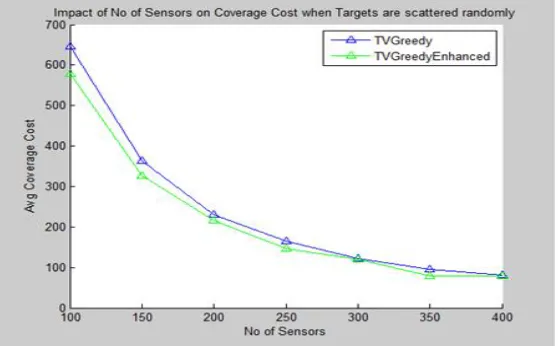
Fig. 7 depicts the performance of TV-Greedy and Enhanced TV-Greedy algorithm when Target are scattered randomly. For both the algorithms, as the number of sensor increases the movement coverage cost decreases. With more sensors, each target can be covered by nearer sensor, which reduces the total movement distance. Enhanced TV-Greedy algorithm incurs less coverage cost compare to TV-Greedy, since in Enhanced TV-Greedy algorithm a single sensor is shared by more than one target thus reduces the movement distance or coverage cost.

Fig. 7. Impact of no of sensors on coverage cost when target are scattered randomly

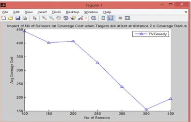
Fig.8. Impact of sensors on coverage cost When Targets are at least at dist 2*coverage radius

2) The Impact of the Number of Target: To evaluate the impact of number of Targets, number of mobile sensors is fixed to 300 and number of targets is varied from 10 to 40. With these parameters, simulations are run in matlab no of times.

Fig. 9 depicts the performance of both the algorithms showing impact of number of target on coverage cost when target are scattered randomly and number of sensors are fixed. In above graph, X-axis represents the number of target varies from 10 to 40 and Y-axis represents the average coverage cost. As shown in the graph, the movement distance increases when the number of target increases.

The reason is that more targets need to be covered as number of target (m) increases, which requires more sensors to be moved and

consequently incur longer movement distance. The enhanced TV-Greedy algorithm as compared to TV-greedy perform better because as the number of targets increases the distance between the targets decreases and chances of sharing the same sensor by the multiple target is increased.

Fig.9. Impact of No. of Targets on Coverage Cost When Targets are scattered Randomly

Fig. 10 represents impact of number of targets on the performance of TV-Greedy algorithm when targets are at distance of twice of its coverage radius from each other. As shown in figure, when the number of targets increases, the coverage cost increases since more target will require more sensors to move to cover it.

B. Performance of ECST-H Algorithm

he performance of ECST-H algorithm is tested based on the positions of coverage sensors generated by TV-Greedy and Enhanced TV-Greedy algorithms. We measured the impact of number of targets and mobile sensors on ECST-H algorithm.

1) Impact of the Number of Mobile Sensors on ECST-H: The following Fig. 11 shows the impact on the movement distance

of ECST-H when number of targets are fixed to m = 30 and number of sensors (n) are varied from 200 to 400 with increment 50.

ECST-H (T) and ECST-H (TE) represents the result of ECST-H when the TV-Greedy and Enhanced TV-Greedy method is used to obtain coverage sensors in the first stage respectively. X-axis represents the number of sensors varying from 100 to 400 and Y-axis represents the movement cost required to connect the coverage cost and sink. As shown in figure, for both the graph, when the number of sensors increases movement cost decreases since with more sensors the closest sensor will move to cover the target, thus reducing the movement of sensor. The possibility of target is already being covered, increased when number of sensors is increased. In Enhanced TV-Greedy algorithm the movement cost is slightly decreased as compared to TV-greedy due to sharing of sensors for coverage.

Fig.11. Impact of sensors on movement distance in ECST-H

2) Impact of the Number of Targets on ECST-H: The following Fig. 12 depicts impact on the movement distance of ECST

-H when number of targets varies from 10 to 40 with increment of 5 and m = 30 and number of sensors (n) remain fixed to 300.

Fig. 12. Impact of no of Target on Movement distance in ECST-H

ECST-H(T) and ECST-H(TE) represents the result of ECST-H when the TV-Greedy and Enhanced TV-Greedy method is used to obtain coverage sensors in the first stage respectively. X-axis represents the number of targets varying from 10 to 40 and Y-axis represents the movement cost required to connect the coverage cost and sink. For both the algorithm (ECST-H(T)and ECST-H(TE)), we observe that as the number of targets increases, movement distance of sensors also increases. This is because more targets require more coverage sensors to cover them. This results in a Steiner tree with more no of Steiner points. The increase in number of Steiner points leads to more number of sensors for movement to connect coverage sensors and the sink. For ECST-H(TE) the cost is slightly decreased since when number of targets increases the possibility of forming target groups and sharing of sensors also increases which reduces the movement cost.

V. CONCLUIONANDFUTURESCOPE

Connectivity (NCON) problem are solved individually. For the TCOV problem, TV-Greedy algorithm is proposed based on Voronoi diagram. For a special case of TCOV where coverage radius is zero, an extended Hungarian method is provided to achieve an optimal solution. In TV-Greedy algorithm, the voronoi diagram of target is used to find the coverage sensor, which determines possible sensors to cover targets and avoid blind competition among the mobile sensors. Since the targets are statically located, the generation of the Voronoi diagram of targets is required only once and re-computation of the Voronoi diagram is not required. Due to grouping of targets based on their proximity to targets, TV-Greedy algorithm minimizes the total movement distance. For the NCON problem, an edge constrained Steiner tree algorithm is proposed to find the location of mobile sensors to connect coverage sensors and sink. Then we use the extended Hungarian to dispatch rest sensors to Steiner points in optimal way. Thus combination of solution to TCOV and NCON offers promising solution to original MSD problem, balancing the load of different sensors and prolong the network lifetime. As a contribution to TV-Greedy algorithm, we have proposed the Enhanced TV-Greedy algorithm which focuses on grouping of targets close to each other and allows sharing of coverage sensor between them to further reduce the movement distance of the sensors. This decreases number of coverage sensors and increases network lifetime.

Simulation experiments done in mat lab have shown that, the solutions based on TV-Greedy algorithms have low complexity and are very close to the optimum solution. The simulation results prove that the performance of Enhanced TV-Greedy algorithm, which is proposed as contribution to this work, is better in performance than existing TV-Greedy algorithm when the targets are scattered randomly in the given task area.

In the future, this work can be extended to address the problem of target coverage and network connectivity in a distributed network. In a distributed mobile sensor network, the main challenge is that, mobile sensors can communicate only with sensors in proximity. Also network changes can be frequent due to sensor failures. For distributed network, the sensor deployment decisions need to be done locally and then applied to whole network. However, the problem is that the algorithms that provide optimal solution locally may not be optimum when looked at in combination with other local solutions. It remains the future work to design a distributed variant of the proposed algorithms to solve the MSD problem in distributed WSNs.

REFERENCES

[1] Zhuofan Liao, Jianxin Wang, Shigeng Zhang, Jiannong Cao, and Geyong Min, ” Minimizing Movement for Target Coverage and Network Connectivity in Mobile Sensor Networks,” IEEE transaction on parallel and distributed system, vol.26, no.7, july 2015.

[2] B. Liu, O. Dousse, P. Nain, and D. Towsley, “Dynamic coverage of mobile sensor networks,” IEEE Trans. Parallel Distrib. Syst., vol. 24, no. 2, pp. 301–311, Feb. 2013.

[3] X. Bai, S. Kumar, D. Xuan, Z. Yun, and T. H. Lai, “Deploying wireless sensors to achieve both coverage and connectivity,” in Proc. 7th ACM Int. Symp. Mobile Ad Hoc Netw. Comput., 2006, pp. 131–142s.

[4] R. Tan, G. Xing, J. Wang, and H. C. So, “Exploiting reactive mobility for collaborative target detection in wireless sensor networks,” IEEE Trans. Mobile Comput., vol. 9, no. 3, pp. 317–332, Mar. 2010.

[5] Aurenhammer, F. and Klein, R. "Voronoi Diagrams." Ch. 5 in Handbook of Computational Geometry (Ed. J.-R. Sack and J. Urrutia). Amsterdam, Netherlands: North-Holland, pp. 201-290, 2000.

[6] Aurenhammer, Franz (1991), "Voronoi Diagrams – A Survey of a Fundamental Geometric Data Structure,". ACM Computing Surveys. 23 (3): 345–405. [7] Robert Sedgewick and Kevin Wayne. Minimum Spanning Tree lecture notes. Computer Science 226: Algorithms & Data Structures, Spring 2007. Princeton