Proposed Mechanism for the Differentiation of
Calcium Signaling in Synaptic Plasticity
II. Evolutionary Algorithms for the Optimization of
Methods in Computational Chemistry
Thesis by
William Chastang Ford
In Partial Fulfillment of the Requirements
for the Degree of
Doctor of Philosophy
California Institute of Technology
Pasadena, California
2012
© 2012
William Chastang Ford
to my Mom, Nicole, Natalie, Mike,
Abstract
In Part 1 of this thesis, we propose that biochemical cooperativity is a
funda-mentally non-ideal process. We show quantal effects underlying biochemical
coop-erativity and highlight apparent ergodic breaking at small volumes. The apparent
ergodic breaking manifests itself in a divergence of deterministic and stochastic
models. We further predict that this divergence of deterministic and stochastic
results is a failure of the deterministic methods rather than an issue of stochastic
simulations.
Ergodic breaking at small volumes may allow these molecular complexes to
function as switches to a greater degree than has previously been shown. We
propose that this ergodic breaking is a phenomenon that the synapse might
ex-ploit to differentiate Ca2+ signaling that would lead to either the strengthening or
weakening of a synapse. Techniques such as lattice-based statistics and rule-based
modeling are tools that allow us to directly confront this non-ideality. A natural
next step to understanding the chemical physics that underlies these processes is
to considerin silicospecifically atomistic simulation methods that might augment
our modeling efforts.
in silicomethods that might be used to describe biochemical processes at the
sub-cellular and molecular levels. While we have applied evolutionary algorithms to
several methods, this thesis will focus on the optimization of charge equilibration
methods. Accurate charges are essential to understanding the electrostatic
interac-tions that are involved in ligand binding, as frequently discussed in the first part
Contents
Abstract iv
List of Figures xvii
List of Tables xix
List of Source Code xxi
I
Quantal Effects in Biochemical Cooperativity and a Proposed
Mechanism for the Differentiation of Calcium Signaling in
Synap-tic PlasSynap-ticity
1
1 Motivation for the Use of Quantal Effectors in Chemical Reaction
Net-works 2
1.1 My Historical Interest in Stochastic Modeling . . . 2
1.2 Simulating More Than Quintillion States of Macromolecular States
on a Personal Computer . . . 3
1.3 Overview of Part I . . . 4
2 Introduction to Rate Theory 6
2.1 Chemical Reaction Theory . . . 7
2.1.1 Mass-Action . . . 7
2.1.2 Rate Theories Derived From Mass-Action . . . 10
2.2 “Reaction Rate Constants” and Non-Ideal Reactions . . . 11
2.3 Reaction Effectors . . . 13
2.4 The Consequences of a Model with Many States: Combinatorial Complexity . . . 14
3 Quantal Effectors on Lattices 16 3.1 Introducing Quantal Effectors . . . 17
3.2 Distinguishing Reactions with Quantal Effectors from Higher-Order Reactions . . . 18
3.3 Cooperativity . . . 19
3.4 Ising Models of Chemical Systems . . . 20
3.5 Rule-Based Modeling for Biochemists . . . 21
3.6 Unification of These Ideas withQuantal Effectors . . . 23
4 Synaptic Plasticity: A Process That Occurs in Small Volumes 26 4.1 Synaptic Plasticity . . . 27
4.2 An Agnostic Approach to Modeling Calcium Calmodulin Kinase II . 27 4.3 Essential Features of a Molecular Switch that Can Differentiate Ca2+ Signals . . . 28
4.3.1 CaMKII is Likely Bistable . . . 29
4.3.2 The Synapse is a System of Limited Resources . . . 29
4.4 What to Look for in the Case Studies . . . 29
5 Method Development 32 5.1 Deterministic Models of Chemical Reactions . . . 32
5.2 Stochastic Simulations . . . 34
5.2.1 Gillespie’s Stochastic Simulation Algorithm . . . 35
5.2.2 Functional Elements of Macromolecules . . . 38
5.3 Additional Details . . . 39
5.3.1 Hardware . . . 39
5.3.2 Software . . . 40
5.3.3 Optimization . . . 40
5.3.4 Data Digitization . . . 40
5.3.5 Deterministic Methods . . . 40
6 Case I. Glycine Protonation 42 6.1 Model Description . . . 44
6.1.1 Standard Scheme . . . 44
6.1.2 Standard Formulation of Glycine/H+ with Differential Equa-tions . . . 46
6.1.3 Standard Formulation of Glycine/H+ with Stochastic Equa-tions . . . 47
6.1.4 Modified Scheme of Glycine/H+ Employing Quantal Effectors 48 6.1.5 Modified Formulation of the Glycine/H+Model . . . 50
6.2 Computational Results . . . 51
6.3 Discussion . . . 52
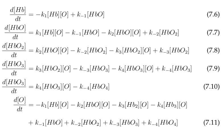
7 Case II: Kinetic and Thermodynamic Models for Oxygen Uptake by Hemoglobin 55 7.1 Kinetic Model . . . 59
7.1.1 Standard Deterministic Formulation of Gibson’s Model of Hemoglobin/O2 . . . 60
7.1.2 Standard Stochastic Formulation of Hemoglobin/O2 as Out-lined by Gibson . . . 62
7.1.3 Modified Scheme of Gibson’s Hemoglobin/O2 Binding Model 63 7.1.4 Computational Results . . . 67
7.2 Thermodynamic Model . . . 67
7.2.1 Standard Deterministic Formulation of Ackers’ Model of Hemoglobin/O2 . . . 71
7.2.2 Standard Stochastic Formulation of Ackers’ Model of Hemoglobin/O2 . . . 73
7.2.3 Modified Stochastic Formulation of Ackers’ Model of Hemoglobin/O2 . . . 75
7.2.4 Computational Size or Summary of Our Models . . . 82
7.2.5 Computational Results . . . 83
7.3 Discussion . . . 85
8 Case III: A Simple Cooperative Dimer and Implications for Calcium
Calmod-ulin Kinase II 91
8.1 The Properties of a Highly Cooperative Protein with Two Binding
Sites . . . 92
8.2 When #A = 1 and #X = 1 . . . 92
8.3 When #A = 2 and #X = 2 and the Idea of Inaccessible States . . . 94
8.4 Revisiting the Ackers’ Model . . . 94
8.5 Ergodic Breaking or Incomparable Ensembles? . . . 96
8.6 How Does This Relate to Calcium Signaling in the Dendritic Spine? . 98 9 Conclusions 100 Appendices 102 Example Source . . . 104
Case I: Glycine Protonation . . . 104
Case II: A Kinetic Model of O2/Hb Association . . . 109
Case IIB: Traditional Deterministic Representation of Hb/O2+2 as pre-sented by Ackers[2005] . . . 116
Case IIB: Traditional Stochastic Representation of Hb/O2+ 2 as pre-sented by Ackers[2005] . . . 122
Case IIB: Modified Stochastic Representation of Hb/O2+2 as presented by Ackers[2005] . . . 132
II
Evolutionary Algorithms for the Optimization of Force-Fields
in Computational Chemistry
141
10 Motivation to Use Evolutionary Algorithms to Optimizein SilicoCode 142
11 Introduction to Evolutionary Algorithms 144
11.1 A Brief History of Evolutionary Algorithm Methodologies . . . 145
11.2 The Chromosome . . . 145
11.3 The Population and Generations . . . 146
11.4 Evolving a Population . . . 146
11.5 Updating, Crossover . . . 147
12 Evolutionary Algorithm Optimization of Charge Equilibration 148 12.1 Optimization Constraints . . . 148
12.2 Initialization . . . 151
12.3 Evaluation . . . 151
12.4 Evolving Our Population . . . 152
12.5 Adaptive Mutation Severity . . . 153
12.6 Mutation Frequency . . . 154
12.7 Training Sets . . . 154
12.8 Final Considerations . . . 155
13 Results 157 13.1 Our Performance . . . 157
13.2 Discussion . . . 159
13.3 Conclusions . . . 167
Appendices 169
Example Source . . . 169
C code for an Evolutionary Algorithm to optimize QEq . . . 169
The integrater for Source Code 9 . . . 181
Index 185
Bibliography 191
List of Figures
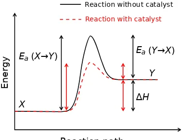
2.1 The relationship between activation energy (Ea) and enthalpy of
for-mation (∆H) with and without a catalyst, plotted against the reaction
coordinate. Ea(X− > Y)and Ea(X− > Y) are the activation ener-gies for the forward and reverse reactions, respectively. The highest
energy position (peak position) represents the transition state. With
the catalyst, the energy required to enter transition state decreases,
thereby decreasing the energy required to initiate the reaction. Wikipedia
[2009] . . . 13
3.1 Lattice model of glycine. The red arrow represents either a
mag-netic field or a very low pH. On the right side of the arrow, we show
the comparable states of glycine. We can model the protonation of
glycine as a function of some force (solvent pH) with the same
equa-tions that we would use to model a ferromagnetic system as shown
on the left. The direction of the arrows are equivalent to a state of
protonation of the lobes of glycine. . . 25
4.1 A zoomed in view of, The Synapse Revealed. Created by Graham
Johnson 2004< graham@f ivth.com >for The Howard Hughes
Med-ical Institute Bulletin . . . 31
6.1 Relationship of Gibbs Free Energy with Cooperativity. Adapted from
Williamson et al. [2008] . . . 43
6.2 Standard formulation of a Chemical Reaction Network representing
Glycine protonation. . . 45
6.3 Modified formulation of a Chemical Reaction Network representing
Glycine protonation. . . 49
6.4 Simulation of glycine protonation. (Red) No charge repulsion. (Blue)
A deterministic model of glycine protonation with charge repulsion.
(Green) A stochastic simulation of glycine protonation with charge
repulsion. Adapted from Figure 2-9a of Wyman and Gill [1990]. . . 54
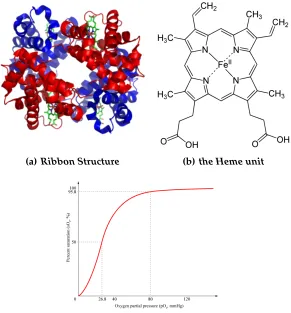
7.1 a) A ribbon structural representation of hemoglobin showing the two
α and twoβ subunits, each with an embedded heme group. b) The
square-planar, top-down view of the primary heme group with Fe(II)
bound in the center of the porphyrin ring. Not shown are the two
apical open coordination sites above and below the ring to complete
the octahedral configuration. c) The characteristic sigmoidal oxygen
uptake curve exhibited by hemoglobin, which is also taken as an
in-dicator of cooperativity. . . 57
(a) Ribbon Structure . . . 57
(b) the Heme unit . . . 57
(c) Prototypical Saturation Plot . . . 57
7.2 Various fits to data obtained from Gibson [1970] . . . 68
7.3 A) A schematic diagram of the possible modes of interaction of hemoglobin with oxygen, according to the model of Adair and interpreted by Imai [1981]. B) Ackers’ detailed model of hemoglobin thermodynamics [2006]. . . 87
7.4 Percentage of hemoglobin bound vs. the total concentration of oxy-gen. The actual oxygen is modified in this plot as the original data did not account for the total oxygen in the system. . . 88
7.5 see next page . . . 89
(a) [Heme]=40nM . . . 89
(b) [Heme]=0.27µM . . . 89
7.5 (cont.) Data fitting of the conceptual model of Ackers and Holt (ref insert 10) to the data of Mills et al. [1976]. The original data is in red and the computer-generated deterministic fits are in blue. . . 90
(c) [Heme]=5.4µM . . . 90
(d) [Heme]=38µM . . . 90
8.1 A comparison of deterministic and stochastic models of a system out-lined in Equations 8.1 and 8.2. Initial conditions are #A=1 and #X=1. . 93
(a) Stochastic Simulation . . . 93
(b) Deterministic Simulation . . . 93
8.2 A comparison of deterministic and stochastic models of a system
out-lined in Equations 8.1 and 8.2. Initial conditions are #A=2 and #X=2. . 95
(a) Stochastic Simulation . . . 95
(b) Deterministic Simulation . . . 95
8.3 see next page . . . 97
(a) 1 Hb@ 38µM [Heme] . . . 97
(b) 2 Hb@ 38µM [Heme] . . . 97
8.3 A comparison of deterministic and stochastic models of a system out-lined in Equations 8.1 and 8.2. Initial conditions are #A=2 and #X=2. . 98
(c) 4 Hb@ 38µM [Heme] . . . 98
12.1 Gameplan . . . 149
13.1 Determination of an initial scaling factor for atomic radii. The scaling factor at minimum error is approximately 1.46. . . 160
13.2 Boxplots of population performance as a function of generation for our initial set of inorganic molecules. . . 161
13.3 Optimization of our inorganic set of molecules. . . 162
(a) Electronegativity . . . 162
(b) Hardness . . . 162
13.4 Boxplots of population performance as a function of generation for our set of organic molecules . . . 163
13.5 Boxplots of population performance as a function of generation for
our set of organic molecules. This plot reproduces the data shown in
Figure 13.4 with outliers excluded . . . 163
13.6 Optimization of our organic set of molecules . . . 164
(a) Electronegativity . . . 164
(b) Hardness . . . 164
13.7 Standard deviations of EA-derived gQEq charges and
quantum-mechanical-derived charges (blue) vs. standard deviations of charges from the
previous model gQEq and quantum-mechanical-derived charges (red) 165
13.8 Mean absolute errors of EA-derived QEq charges and
quantum-mechanical-derived charges (blue) vs. mean absolute errors of charges from the
previous model QEq and quantum-mechanical-derived charges (red) . 166
List of Tables
6.1 A standard tableau depicting the reactions required to determine the
speciation of glycine as a function of pH. . . 46
6.2 A standardized formulation for glycine protonation vs. pH. The data
elements are valued from zero to infinity. . . 46
6.3 A “rule-based” type reaction scheme for glycine/H+ . . . 50
6.4 A modified formulation of the data model for glycine protonation . . 50
7.1 Kinetic and thermodynamic data obtained by Gibson for the
stoichio-metric reaction of oxygen with hemoglobin . . . 60
7.2 A standard formulation of the reaction scheme of Hb/O2 by Gibson . 60
7.3 A standardized formulation for Gibson’s oxygenation of hemoglobin.
The data elements are real valued from zero to infinity. . . 61
7.4 A standardized formulation for Gibson’s oxygenation of hemoglobin.
The data elements are integers valued from zero to infinity. . . 63
7.5 The modified formulation for hemoglobin oxygen complexation states 64
7.6 The standard formulation for hemoglobin oxygen complexation states 76
7.7 This table provides a numerical comparison of the relative
complex-ity in the problem formulations for two protein systems exhibiting
kinetic and thermodynamic cooperativity. The numbers separated by
a slash (/) are for either the bidirectional or unidirectional case, in
that order. . . 83
7.8 A modified formulation of the reaction scheme of Hb/O2by Gibson . 84
7.9 A modified formulation of Ackers’ Hb/O2 . . . 84
7.10 Deterministic fits of the mechanism of Ackers and Holt [2005] to the
data of Mills et al. [1976] . . . 85
11.1 A binary chromosome . . . 146
11.2 A real valued chromosome . . . 146
12.1 An example of our population of real-valued chromosomes whose
value represents a scaling rather than a specific value . . . 151
12.2 Data from Rapp´e & Goddard [1991] . . . 152
12.3 Initial training cases . . . 155
13.1 Original parameters and our optimized values for electronegativity . . 158
13.2 Original parameters and our optimized values for hardness. . . 159
Algorithms and Source Code
1 A snippet of code from Source Code 4 . Line 1 converts a molar
quantity to discrete values. . . 51
2 A snippet of code from Source Code5. This snippet focuses on the
reaction rate function that implements Gibosn’s findings. The
vol-ume of the box is calculated such that 1µMof hemoglobin equals 1
hemoglobin in the system. . . 65
3 A snippet of code from Source Code8. The following code
imple-ments Acker’s cooperative scheme of Hb/O2+2 complexation. . . 78
4 Glycine protonation represented as a system of ordinary
differen-tial equations, the stochastic simulation algorithm, and “rule-based”
techniques . . . 104
5 Gibson’s kinetic model of Hb/O2, applied to his own data as
re-ported in [1970] . . . 109
6 A deterministic model of Hb/O2 dynamics as presented by Ackers
KinpySrinivasan . . . 116
7 A standard stochastic model of Hb/O2 dynamics as presented by
Ackers . . . 122
8 A modified stochastic model of Hb/O2 dynamics as presented by
Ackers . . . 132
9 C code for an Evolutionary Algorithm to optimize QEq . . . 169
10 The integrater for Source Code 9 . . . 181
Part I
Quantal Effects in Biochemical
Cooperativity and a Proposed
Mechanism for the Differentiation of
Calcium Signaling in Synaptic
Chapter 1
Motivation for the Use of Quantal
Effectors in Chemical Reaction
Networks
1.1
My Historical Interest in Stochastic Modeling
My motivation for the work contained in Part I of my thesis started before I
matriculated at Caltech. I spent two years studying stochastic chemical reaction
networks under the late Dr. Joel Stiles at the Pittsburgh Supercomputing
Cen-ter. Joel was a co-author of a software package used to perform particle-based
reaction-diffusion simulations of biochemical systems in arbitrarily complex
three-dimensional space. Joel called this “Microphysiology.”
Much of my PhD has been spent developing methods in computational
chem-istry. As an undergraduate, I began working with a simulation package called
MCell, a stochastic reaction-diffusion simulation package. I transitioned into
de-veloping methods of stochastic simulation and optimization that will be discussed
later in Part II of this thesis.
1.2
Simulating More Than Quintillion States of
Macro-molecular States on a Personal Computer
An early project that I worked on involved modeling a ”full-state” model of
calcium / calmodulin / calcium calmodulin kinase II. This model, as conceived,
contained more than 1019states and was the most complex (high number of states
vs. the number of molecular constituents) proposed model of a biochemical
sys-tem that I was aware of. I devised of a method to model it that is similar to past
methods applied to hemoglobin. I initially implemented this method as a
wrap-per around MCell, a reaction diffusion simulating code. I treated the system as if
hemoglobin were in a lattice, and I manipulated reaction rates as a function of the
states of the other subunits. The rate law for the nodes of the lattice is a function
of the occupation of the subunits of CaMKII’s neighbours. This is analogous to the
”lattice-based” methods of Terrance L. Hill and other theoretical chemists.
In the process of building these models of Ca/CaM/CaMKII, I became aware
that other modelers were doing something similar to what theoretical chemists had
done in the past, but without explicitly building upon their work. “Rule-based
modeling” has reformulated a solution to patch-up the problem of combinatorial
explosions without addressing its cause, our formulation of solutions. I will
ad-dress the fact that we are growing out of the simplistic description of chemical
reac-tion networks that mass-acreac-tion requires. This is the impetus to develop a language
to explicitly describe chemical reactions that are governed by non-ideal
tions as quantal chemical reactions. We need to develop a more general language
and understanding of quantal chemical interactions that is not domain-specific, or
taught only to graduate level chemists, physicists, or computer scientists.
1.3
Overview of Part I
In Chapter 2 of this thesis, I will review our recent standard treatments of
chem-ical reaction networks. In Chapter 3, I will then draw similarities between the use
of lattice statistics and rule-based modeling for the simulation of biochemical
sys-tems.
In Chapter 4 I will discuss a biological system where our later findings might
provide useful insight.
In Chapter 5, I will review the computational methods that I use that should be
accessible to undergraduate students. I will also propose that we should not look
toward differential methods as a reference point by which to base the validity of
the use of stochastic models to represent systems that are inherently stochastic.
In the following chapters, I will present several case studies that give insight
into a general treatment of non-ideal systems. When possible, I will refer to
fea-tures that are analogous to other formulations. In the first case, the pH-dependent
protonation of the zwitterion of glycine is modeled, and the various solutions are
compared.
In the second case, the complexation of four dioxygen molecules by hemoglobin
is modeled in an effort to account for the apparent cooperative relationship, or the
enhanced binding affinity with respect to the successive uptake of oxygen, that is
observed experimentally between the four different subunits of the hemoglobin
molecule. In the third case, I will lay out the foundation for building “toy models”
of calcium (Ca2+), calmodulin (CaM), and calcium-calmodulin kinase II (CaMKII).
I will subsequently refer to these as Ca2+ / CaM / CaMKII models as they were
the impetus for the other case studies. I first witnessed the quantal effects of
coop-erativity when modeling a system of Ca2+/ CaM / CaMKII. I initially described it
in a candidacy report that I wrote in the beginning of 2009.
Chapter 2
Introduction to Rate Theory
The idea of a rate constant is a misconception. Enzymes can catalyze
reac-tions after association with their substrate. The association of a non-competitive
inhibitor, often distal to an active-site of a protein, can decrease the reaction rate
of that protein. Even the state of local subunits of a macromolecule may affect the
reactivity of other subunits. Though it is glossed over, this phenomena is non-ideal
and bound by those consequences. In this portion of my thesis, we will develop the
idea of quantal effectors as they apply to cooperative chemical reactions. The
ma-jor proposition of this work is that although we can model large systems with the
equivalent of many quadrillion states, we are still bound by the fact that we are
modeling quantal effects.
In collision theory of gas-phase kinetics, there is the assumption that in a dilute
gaseous environment, the propensity for the collision or association of an A-B pair
to result in a reaction is not affected by the existence of other non-reacting elements.
At the same time, it states that the rate of this reaction is governed by AeEART. In
biochemistry, EA is known to be affected at times by non-reacting molecules (for
example, neighboring subunits in a macromolecular complex). Transition state
theory deals with this complication by including the addition of a non-reacting
effector in another reaction, thereby allowing a reaction to proceed with a different
EA.
We circumvent the assumption that reactants cannot be affected by non-reactants
by including the various combinations that might affect a reaction rate explicitly.
Alternatively, instead of explicitly stating each and every combination that might
affect a reaction rate, we implement reaction-rate functions, such as the Arrhenius
equation or a “rule-based modeling” type of relationship.
2.1
Chemical Reaction Theory
2.1.1
Mass-Action
For a detailed account of the history of the law of mass action see Lund [1965].
Rate of Reaction∝k[A][B]
where kis the reaction rate constant, [A] is the concentration of one reactant, and
[B] is the concentration of another reactant in a bimolecular reaction.
The following relationship is relevant and can be found in MacQueen [1967].
∆Gθ =−RTlogeK (2.1)
∆Gθ =∆Hθ−T ∆Sθ (2.2)
K = exp −
∆Gθ RT
= exp−∆H θ
RT exp ∆Sθ
R (2.3)
The particulars of the function are not as important as gaining an appreciation for
the form of the function (for further details see Wright [2004]).
Chemical reactions have been described thermodynamically using
Maxwell-Boltzmann statistics for more that a century. Maxwell-Maxwell-Boltzmann statistics are
de-rived from the theory that reactions can be broken up into specific classes and
described by the stoichiometry or the order of the reaction Gillespie [1976].
• For example:
– Zero Reactants / Zeroth-Order Reaction / “Birth Processes”
∗ → reaction products
rate =k.
– One Reactant / First-Order Reaction/ “Unimolecular Processes”
Sj → reaction products
rate =k[Sj].
– Two Reactants / Second-Order Reaction/ “Bimolecular Processes”
Sj +Sk → reaction products(j 6=k)
rate =k[Sj][Sk]
2Sj → reaction products
rate =k[Sj]2.
– Three Reactants / Third-Order Reaction/ “Termolecular Processes”
Si+Sj +Sk → reaction products(i6=j 6=k)
rate =k[Si][Sj][Sk]
Sj + 2Sk → reaction products(j 6=k)
rate =k[Sj][Sk]2
3Sj → reaction products
rate =k[Sj]3.
While higher-order reactions are theoretically possible, we typically consider
reactions to be decomposable into zero-, first-, or second-order processes. The
the-ory behind this is that it is improbable for more than two independently diffusing
particles to interact or collide with one another at the exact same time. For
dently diffusing particles, this is most likely true. In the case of macromolecules,
reactive units tend to diffuse together.
Various updates that have been made to the initial theories have brought us
closer to modeling the physical realities of chemical systems.
2.1.2
Rate Theories Derived From Mass-Action
Consider the following equation to represent the general form for a reaction
rate function.
k= (pEF)e−RTE (2.4)
k= (pEF)e−(ERT1+E2)
k= (pEF)e−RT∆He ∆S
R
Equation 2.4 has components pEF, E, R, T, ∆H, and ∆S, which equal the
pre-exponential factor, energy, a gas constant, temperature, change in enthalpy, and
change in entropy, respectively. The form of this function is seen in the Arrhenius
equation, collision theory, and transition state theory.
lnk =−(Ea
RT) + lnA
k =Ae(−RTEa) (Arrhenius equations)
k=pZe(−RTEa)
k=PrZe(−
Ea
RT) (Collision theory)
k =κkT h
Q6=∗
QxQyze (−E0
RT) (Transition state theory)
2.2
“Reaction Rate Constants” and Non-Ideal Reactions
Above, I use quotes when discussing rate constants because the term is a
mis-nomer and interferes with our ability to talk about non-ideal reactions in a more
general context. Reaction rates are not always constant and should be thought of
as functions that are affected by both macroscopic factors and microscopic factors,
akin to extrinsic and intrinsic properties of systems.
The most famous rate function is the Arrhenius equation:
k=Ae−RTEa (2.5)
wherekis the reaction rate constant,Ais a pre-exponential term,EAis the energy
of activation,Ris the gas constant, andT is the temperature. The Arrhenius
equa-tion treats the rate of the reacequa-tion as a funcequa-tion of temperature and can be thought
of as a reaction rate equation or as a “rule” that describes the relationship of rate
and temperature. “Rule” is a term coined in rule-based modeling while “reaction
rate equation” is a more descriptive term. Typically, chemists do not implement
this function consistently.
• Often when chemists consider a change in temperature, they explicitly
in-voke this equation or similar equations. This is because it is the same reaction
under different conditions. The explicit treatment results in understanding that
the rate of reaction is a function of temperature.
• Often when chemists consider a change of energy of activation, they ignore
the dynamic nature of reaction rates. An example of this is the treatment
of auto-catalytic systems such as hemoglobin/O2. We explicitly elaborate
out all non-ideal effects that lead to changes in reaction rates. In doing so,
we treat the binding ofO2 to hemoglobin’s four sites as as many as sixteen
different reactions.
A non-ideal reaction exhibits behavior that allows other molecular elements
that are neither reactants or products to affect its rate of progression. These
non-ideal interactions occur at the individual level and are not directly compatible with
common calculus-based models. This class of interactions that are discrete in
na-ture can be described by mass-action if every non-ideal interaction is elaborated
out. This treats a single complicated reactions as a set of reactions. For highly
non-ideal systems, this results in a large number of simple reactions. This is termed
combinatorial complexity.
Rule-based modelers often state that their method resolves the combinatorial
complexity of chemical reactions. This definition speaks to treating the symptoms
of a problem without realizing the fundamental cause. We will discuss this further
in the section on “rule-based modeling.”
2.3
Reaction Effectors
Reaction path
E
n
e
rg
y
X
Y
(X→Y)
Ea Ea(Y→X)
∆H
Reaction without catalyst
[image:34.612.230.419.174.318.2]Reaction with catalyst
Figure 2.1: The relationship between activation energy (Ea) and enthalpy of for-mation (∆H) with and without a catalyst, plotted against the reaction coordinate. Ea(X− > Y) and Ea(X− > Y) are the activation energies for the forward and reverse reactions, respectively. The highest energy position (peak position) rep-resents the transition state. With the catalyst, the energy required to enter transi-tion state decreases, thereby decreasing the energy required to initiate the reactransi-tion. Wikipedia [2009]
In biochemistry, there are promoters and inhibitors of chemical reactions that
affect the rate of reactions, but do not necessarily interact directly with the reacting
elements. We will refer to this class of molecules and molecular domains as
“ef-fectors”. They may affect the reaction coordinate of reacting biological molecules
by altering the activation energy, as depicted in Figure 2.1. The Arrhenius
equa-tion (2.5) shows us that a change inEAleads to a change in the rate constant of a
reactionk.
Enzymes, a subgroup of biological effectors, are the biological equivalent of
catalysts. Figure 2.1 illustrates an example of how one might describe the action
of a catalyst. Enzymes and catalysts are modeled as if they lower the activation
energy of a reaction.
2.4
The Consequences of a Model with Many States:
Combinatorial Complexity
For more than a century, rate equations have been used to describe systems
by posing questions in the following form: “How much of a molecule in some state
X exists at time T?” This is the result of the population-based framework that is
required when invoking the law of mass-action. Biochemists and biophysicists
have sought to use these models to help understand a variety of processes, from
gene transcription, to oxygen delivery to tissues, to cell signal transduction.
The molecules that are modeled in these processes exist in various states, and
each state is typically represented by an individual data element. For example,
a molecule bound to a substrate exists in a different state than a molecule of the
same type in its unbound form or bound to a different substrate. Furthermore,
macromolecules in which multiple subunits act as effectors of other subunits are
often described as a combination of the individual states of the subunits, such that
the number of states of the macromolecule is equal to:
(possible states ofsubunit1)×(possible states ofsubunit2). . .×(possible states ofsubunitn).
Thus, a homo-oligomer can to be described byabdata elements, whereaequals
the number of states in which a single subunit can exist, andbequals the number of
subunits in a macromolecule. One example of this is cooperative binding, where
inter-subunit interactions allow for increasing binding affinity upon subsequent
binding events.
Modelers have grown accustomed to building models in which the number
of data elements (i.e., the model’s data-space) equals the number of states of all
molecules modeled in the system (i.e., the model’s state-space). Following this
dogma, as the number of subunits in an oligomer increases, the number of data
elements needed to describe its states increases exponentially. This is sometimes
referred to as a combinatorial explosion (ab). In this work, we present a framework
in which we are able to represent the full state-space of approximately ab states
with a significantly smaller data-space, a×b. In the following chapters we will show that the combinatorial complexity is a function of the theory of mass action
rather than a truth of real chemical reaction networks.
As an aside: It is more impressive to model chemical reaction networks
with-out defining reactants, products, effectors, and reactions. By employing reactive
molecular dynamics force-fields such as Reaxff (van Duin et al. [2001]), one can
model complex biochemical systems without predefining many of the features
re-quired in standard or modified models of chemical reaction networks. Code for
optimization of Reaxff will be provided at the end of the second part of this thesis.
Chapter 3
Quantal Effectors on Lattices
In this chapter, we introduce the terminology used to describe molecular
ele-ments that exhibit explicitly non-ideal behavior. We define these terms here so that
we might describe the quantal effects that we see in future chapters. We will
in-troduce quantal effectors that behave in an explicitly discrete manner. We will also
discuss their early description as cooperative effectors and how they were treated
in the mass-action framework. Next we will touch on statistical mechanics,
specif-ically lattice theory as it has been applied to hemoglobin to model cooperative
effects.
Following this discussion of discretization of hemoglobin subunits to points on
a lattice, we will discuss how these ideas have been re-framed and extended by
rule-based modelers. Finally, we will attempt to unify the insights made toward
the understanding of hemoglobin with a general theme that we have revisited:
that we do not have an appropriate language to describe molecular elements that
affect reactions in a discrete manner, but are neither reactants nor products.
3.1
Introducing Quantal Effectors
Cofactors, promoters, and non-competitive inhibitors can and should be
con-sidered “effectors” of reactions. We have excluded competitive inhibitors from
this list because they directly interact with the binding site of at least one of the
reacting molecules and, therefore, could play a very different role than effectors.
A very important subclass of effectors are the subunits/domains of molecules and
macromolecules that affect the reactivity of other subunits/domains. We will refer
to these as “quantal effectors”.
Quantal effectors are molecular entities that are explicitly non-ideal. Naming
these elements quantal effectors gives the user insight into the quantal behavior
that may become apparent under certain conditions. An alternative name that is
equally or more apt is non-ideal effector. Such a term is important because it is
not domain-specific, and it provides insight into general truths. Domain-specific
terms—such as lattices, agents, and rules—have specific meanings that are difficult
to distinguish from the methods with which they are associated.
Since the early 20th century, we have been aware of complex reaction
dynam-ics shown by molecular complexes. In 1925, Adair showed that hemoglobin has
multiple binding sites for oxygen and that these sites potentiate one another when
bound. While the reacting dynamics of hemoglobin can be coaxed into a
mass-action type of model, it is non-ideal in that hemoglobin subunits autocatalyze one
another in a non-ideal manner that is only partially governed by mass-action, as
quantal effectors.
3.2
Distinguishing Reactions with Quantal Effectors
from Higher-Order Reactions
Adding a quantal effector to a reaction may appear to be equivalent to
increas-ing the molecularity of the reaction, but it is explicitly not equivalent. The quantal
effector is more likely to affect only a small subset of the ensemble.
Consider a termolecular reaction that is ideal in that it obeys mass-action
dy-namics. Termolecularity implies that the reaction occurs due to the diffusion of
three particles colliding with one another at the same instant of time. There are
two points to consider here:
• The probability of collision is much lower for three particles diffusing in a
solution than it is for a macromolecule with multiple sites and a particle
dif-fusing in a solution.
• In a reaction, any elements that are representative members of the class of
reactants may interact with one another. Often in macromolecules subunits
maintain their associations, resulting in less promiscuous reaction schemes.
Ising models of chemical systems tend to maintain their node/connection
structure.
Therefore, quantal effectors should be considered more likely and and less
promis-cuous than true higher-order reactions.
3.3
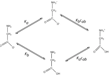
Cooperativity
Cooperative binding requires that a molecule, such as hemoglobin or glycine,
has more than one binding site. In Binding and Linkage [1990], Wyman refers to
the phenomena of charge repulsion between the protonation sites of glycine as
“linkage” rather than “negative cooperativity” based upon the belief that an
al-losteric shift is required for a cooperative event to occur. It should be noted that
the allosteric model of hemoglobin/O2that was proposed by Monod, Wyman, and
Changeaux in [1965] earned them a Nobel prize. In this thesis, we are not
attempt-ing to challenge the notion of allostery beattempt-ing essential to hemoglobin cooperativity.
We do not wish to use multiple words to describe phenomena whose
mathemat-ical treatment would be equivalent. Therefore, we will lump “cooperativity,”
“al-lostery,” “causal rules,” “linkage,” and “coupling” into one general phenomena
governed by non-ideal interactions. We call this phenomena “cooperativity” out
of respect for its early description (Adair [1925b]).
We generalize cooperative processes to be those reactions that are explicitly
non-ideal, in that an element that is not a product or reactant affects the progress
of a reaction. Again, we refer to these elements as quantal effectors. For example,
the charge repulsion that a protonation site of glycine experiences due to the other
site being occupied is a negative cooperative effect. In this case, the protonated
terminus that is not taking part directly in the subsequent protonation inhibits
the reaction. Conversely, if the binding of the ligand oxygen at one binding site
of hemoglobin increases the affinity for another oxygen at a different site on the
same macromolecule, this is considered to be positive cooperativity. The quantal
effects in this case are the other subunits, meaning that for each binding site of
hemoglobin, there are three quantal effector sites that might affect reactions at that
site in an explicitly non-ideal manner.
At this point, we can relate the idea of cooperativity back to some concepts of
rate theory that were presented earlier. In the reportEnergetics of Subunit Assembly
and Ligand Binding in Human Hemoglobin [1980], Gary Ackers suggests that “the
dominate driving forces for cooperativity may be a combination of hydrogen bond
formation, preferentially stabilizing the tetramer with large negative∆Sand small
∆H, and Bohr proton release, yielding large positive enthalpies and moderate but
negative entropies”.
3.4
Ising Models of Chemical Systems
In 1925, Ising proposed a model for the study of ferromagnetic systems. The
Ising model has since been applied to many fields, including biochemistry and
computational neuroscience (Hopfield [1982]). Lattice models of cooperative
sys-tems typically break up the molecular subunits of a macromolecule into nodes on
a lattice. The points on a lattice have independent probabilities of transitioning
until they are connected. Once connected, the states are either positively or
neg-atively coupled, and the states of connected nodes are affected by the “coupling
coefficient”. An illustration depicting the relationship of Ising models to a lattice
model of a molecule, glycine, is presented as Figure 3.1.
While there are many papers that treat cooperative systems using lattice
meth-ods, we will focus on a single paper that models hemoglobin as a set of points on
a lattice using the relationships proposed by Pauling [1935]. Chay and Ho [1973]
use lattice statistics to model hemoglobin as a two-dimensional Ising model with
N = 4. They modeled different cooperative relationships between the subunits of
hemoglobin in an attempt to elucidate the underlying mechanisms of its
coopera-tivity. Their work is similar to what Pauling did in 1935 using mass action
equa-tions. The models of Chay are explicit examples of treating cooperative
relation-ships as non-ideal processes. The non-ideal relationrelation-ships represent the cooperative
and causal relationships between molecular subunits of a macromolecule.
3.5
Rule-Based Modeling for Biochemists
Rule-based modeling is a field of simulation that, by citation, seems to derive
from Gillespie’s stochastic simulation algorithm [1976, 1977]. I contend that they
also derive from the understanding of chemical physics that underlies lattice
statis-tics of cooperative macromolecules. Both lattice statisstatis-tics and rule-based modeling
break up macromolecules into their constituent parts and explicitly consider the
relationships between them. It is interesting that few, if any, rule-based
model-ing packages refer to the lattice-based statistical methods that they mirror. Lattice
statistics is a field that is still active, and it is faced with issues of intractability that
could be resolved with solutions from rule-based modeling.
Many rule-based modeling packages do not attempt to give their rules a
phys-ical basis. Moleculizer (Lok and Brent [2005]) is a package that does explicitly
attempt to employ physical reasoning for its rules. For example, Lok and Brent
[2005] presented a stochastic model for the effects of oligomerization on the
chem-ical reaction rates of the corresponding monomer using a classchem-ical collision theory
formulation as follows:
cµ=V−1πd212(8kT /πm12)1/2exp(−uµ/kT) (3.1)
where cµis the stochastic reaction rate parameter, m12is the adjusted mass,kis the
Boltzmann constant,d12 is idealized collision cross-section diameter, V is the
vol-ume of the system, anduµis analogous to the energy of activation. The approach
taken by Lok and Brent is based on classical molecular collision theory.
One oddity of rule-based modeling is that the different camps of rule-based
modelers do not have a unifying language to talk about the formulation of their
models. I began rule-based modeling in 2006 without knowledge of the
commu-nities of rule-based modelers that began developing around 2004. My first models
involved pausing stochastic simulations, altering their rates as a function of the
states of the subunits of a “toy hemoglobin”, and then restarting the simulation.
When I discovered the rule-based modeling communities, I was frustrated that I
could not clearly determine if we were doing analogous work.
This is because the language that the communities use is either partially
self-generated (Lok and Brent [2005]), rooted in abstract computer science (Danos and
Laneve [2004]), or both (Blinov et al. [2004]). For example, Moleculizer (Lok and
Brent [2005]) refers to molecular subunits asmols, while Kappa(κ) (Danos and
Lan-eve [2004]) and BioNetGen (Blinov et al. [2004]) refer to subunits asagents. This is
part of the impetus to create a unified language to describe these non-ideal
rela-tionships that lead to cooperative behavior.
Furthermore, various pieces of software have been developed to perform
rule-based modeling without presenting generalized outlines and derivations of their
methods, in the vein of what Gillespie has presented [1976, 1977]. These programs
appear to treat molecules as individuals, rather than populations. This is an
im-portant point because they are essentially reversing the step in many mass-action
based derivations of chemical reaction theory that break up complicated reactions
into several simple reactions to fit into a population-based framework. This is a
relevant point that is seemingly absent in rule-based modeling literature.
3.6
Unification of These Ideas with
Quantal Effectors
To unify these ideas, it is important to look at the fundamental truths that these
methods are trying to address. The language that we use to describe chemical
reac-tions is limited by the view that reacreac-tions contain only reactants and products. In
the 1970s, theoretical chemists, and more recently rule-based modelers, redefined
rate laws to include the state of particles that are neither reactants or products. A
fundamental feature of these particles is that they affect the reaction rate in a
fun-damentally non-ideal manner that is quantal in nature. Hence, we refer to them as
“quantal effectors”.
Furthermore, at very small numbers, the simple non-ideal relationships
be-tween these complex elements can lead to behavior that is similar to
ergodic-breaking. In quantum mechanics, quantal effects are a cause of ergodic-breaking,
given that theensemblesconsidered are comparable. This again supports the name
quantal effectors, as it is informative and corrects the misconception that
determin-istic and stochastic treatments should always converge. In this thesis, we will
de-fine the quantal effector limit beyond which one could safely expect
macroscopic-like behavior.
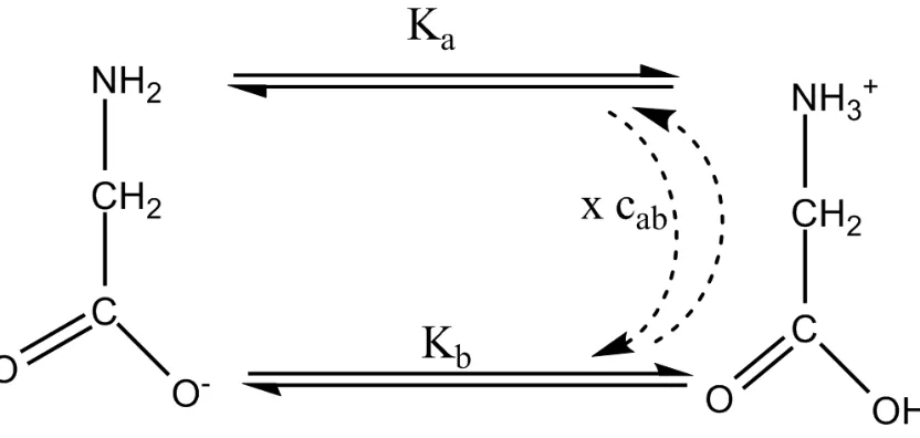
NH
3+-CH
2
-
COOH
NH
3+-CH
2
-
COO
-NH
2-CH
2-
COOH
NH
2-CH
2-
COO
-Figure 3.1: Lattice model of glycine. The red arrow represents either a magnetic field or a very low pH. On the right side of the arrow, we show the comparable states of glycine. We can model the protonation of glycine as a function of some force (solvent pH) with the same equations that we would use to model a ferro-magnetic system as shown on the left. The direction of the arrows are equivalent to a state of protonation of the lobes of glycine.
[image:46.612.171.418.198.473.2]Chapter 4
Synaptic Plasticity: A Process That
Occurs in Small Volumes
While much of this thesis will discuss hemoglobin and glycine, it is not
bio-physically realistic to think about these molecules as naturally existing in small
volumes with limited availability of ligand. We use them as tools to understand
biological cooperativity on the smallest scale because they are useful tools in
de-veloping an understanding of cooperative biological processes that occur in small
volumes. Having been a neuroscientist for the past 15 years, I have my biases.
Synaptic plasticity is a process that occurs in small volumes and is thought to be
at least partially mediated cooperative processes. A key component in synaptic
plasticity is the differentation of low Ca2+ for the weakening of the strength of a
synapse and high Ca2+ influx for the strengthening of synaptic connections. In
subsequent chapters, I will use the life molecule, hemoglobin, to understand the
mind molecule, calcium calmodulin kinase II (CaMKII).
4.1
Synaptic Plasticity
To the best of our knowledge, the synapse is the center of learning and memory
(Bliss and Lomo [1973]). The synapse is a subcellular structure that has both a
small volume and is diffusionally restricted under certain conditions (Bloodgood
and Sabatini [2005], Sabatini et al. [2002]).
A beautiful rendition of the synapse—“The Synapse Revealed”—can be seen in
Figure 4.1.
4.2
An Agnostic Approach to Modeling Calcium
Calmod-ulin Kinase II
Calmodulin (CaM), a ligand of CaMKII, has two lobes, the N-terminal and
C-terminal lobes. Each lobe can bind up to two Ca2+ ions, and even partially ligated
CaM has the ability to phosphorylate CaMKIIin vitro(Shifman et al. [2006]).
There-fore, CaM can exist in at least nine different states, as the two lobes can each exist in
the states of unbound, singly bound, and doubly bound to calcium. Each species
of CaM can interact with a subunit of the dodecameric macromolecule CaMKII.
It has been reported that CaMKII itself can be phosphorylated in many
posi-tions including the following: T253 (Dosemeci and Reese [1993]), T286 (Lai et al.
[1987], Miller and Kennedy [1986]), T305 (Colbran and Soderling [1990]), and T314
(Colbran and Soderling [1990]). Interestingly, dynamics that are apparentin vitro
(Miller and Kennedy [1986]) may not exist in vivo(Mullasseril et al. [2007]). The
system is further complicated by the fact that that CaMKII exists as a
heteroge-neous mix of more than one isoform (α and β) in the synapse. While I have
pre-viously generated large models of CaMKII including many, but not all of these
features, a true elucidation of a robust mechanism by which the synapse might
differentiate between various calcium signals has not been shown.
4.3
Essential Features of a Molecular Switch that Can
Differentiate Ca
2+Signals
Much of the work in synaptic plasticity research is directed toward
understand-ing the switch-like behavior of CaMKII (Miller and Kennedy [1986]). In this thesis,
we propose that the key to understanding how CaMKII might ignore weak
Cal-cium signals while reacting to strong ones is a ubiquitious feature of positively
cooperative molecules under a situation of limited resources. Furthermore, we
agree with Lisman in that the “ensemble” that many bench-top experiments create
is incomparable to the “ensemble” that exists in the cell (Sanhueza et al. [2011]).
We hypothesize that two key features of the Ca2+/CaM/CaMKII complex,
bista-bility of CaMKII and limited resources of Ca2+, allow for signaling differentiation
that in isolation is a thermodynamically robust bench-top experiment.
4.3.1
CaMKII is Likely Bistable
In 2000, Zhabotinsky showed that CaMKII exists primarily in one of two states.
In order for one to apply experimental results to a system including CaMKII to
infer features of its activity in the synapse, the experiments should be performed
under conditions that would be equivalent in size and molecular composition to
the synapse. We will show that it is possible to predict non-ensemble behavior
of CaMKII in the synapse based upon a simple understanding of cooperativity
due to quantal effects mediated by quantal effectors. If one were to consider a
synapse to be comparable to a bench-top experiment, this quantal behavior would
be comparable to ergodic breaking.
4.3.2
The Synapse is a System of Limited Resources
There are not many Ca2+ ions in the synapse (Sabatini et al. [2002]). A low
maintained local level of Ca2+ should be sufficient to circumvent the activation of
CaMKII, even at local concentrations that might be thought sufficient to activate
it. There are many analogies that can be drawn between a cooperative molecule in
the synapse and the quantum mechanical treatment of a particle in a box.
4.4
What to Look for in the Case Studies
1. In Case I, glycine is useful because in our modified lattice model, it is directly
analogous to spin pairing of electrons in a shell.
2. In the first half of Case II, Gibson’s kinetic model of hemoglobin is discussed
briefly to show that we can match kinetic as well as thermodynamic data.
3. In the second half of Case II, Ackers’ thermodynamic model of hemoglobin is
discussed to exemplify the scope of the problem. This system shows quantal
behavior of positively cooperative models in small spaces.
4. In Case III, we will conclude with a “toy” model to show what the sufficient
conditions are for non-ensemble-like behavior, and how this relates to the
aforementioned points.
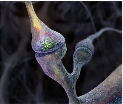
Figure 4.1: A zoomed in view of, The Synapse Revealed. Created by Graham Johnson 2004< graham@f ivth.com >for The Howard Hughes Medical Institute Bulletin. Mr. Johnson’s illustration of two synapses. The green spheres represent synaptic vesicles and are located in the presynaptic side of the synapse. The side directly opposing the presynaptic side is referred to as the postsynaptic side of the synapse in this case it is also known as a dendritic spine.
Chapter 5
Method Development
In this chapter, we initially discuss traditional calculus-based and stochastic
methods of modeling chemical reaction networks. We then review and elaborate
on an alternative method of stochastic modeling that has been named rule-based
modeling.m Rule-based modeling was built for biochemists, but it often employs
language that makes it inaccessible to biochemists and computational chemists.
In this chapter, we redefine rule-based modeling for experimental and theoretical
chemists. We do this without difficulty by referring to the history of fundamental
components of rule-based modeling that existed before the coining of the term
rule-based modeling for biological systems. Finally, we outline the theme by which
rule-based modeling can be unified with existing chemical theory and its likely
niche in the greater context of computational chemistry.
5.1
Deterministic Models of Chemical Reactions
In the late 19th century, scientists began to create mathematical models of the
evolution of chemical species in reactions using mass-action (Lund [1965]). The
use of calculus-based methods, such as differential equations, to model chemical
species were a natural extension of this work. This type of modeling is termed
de-terministic because, given a model and a set of initial conditions, it will reproduce
the same results on repeated trials. This is not the case for stochastic models which
will be discussed later.
A standard deterministic approach is employed to provide a solution to a
sys-tem of coupled differential equations that are defined by a detailed chemical
reac-tion mechanism. Let us consider the stoichiometric reacreac-tion of A with B forming a
discrete reaction product C:
A+BGGGGGGBFGGGGGGk1 k−1
C (5.1)
where k1 is the forward second–order “rate constant” andk−1 is the reverse
first-order “rate constant.” The equilibrium constant for the reaction of Equation 5.1 is
given by the law of mass-action, as follows:
K1 = k1 k−1
. (5.2)
The complete kinetic description of the simple reaction of Equation 5.1 is as
fol-lows:
dA
dt =−kon[A][B] +kof f[C] (5.3) dB
dt =−kon[A][B] +kof f[C] (5.4) dC
dt =kon[A][B]−kof f[C] (5.5)
where [A]and[B]are the concentrations of reactants and[C]is the concentration
of the reaction product. In a conventional formulation, the concentration units for
an aqueous-phase reaction are expressed in units of moles per liter (i.e., mole L−1
or M); for a homogeneous gas-phase reaction, they are expressed in units of the
numbers of molecules per cubic centimeter (i.e., molecules cm−3). The forward
rate constant kon then has the corresponding units of either L mole−1 s−1 or cm3
molec−1 s−1, while the reverse rate constantk
of f has units of s−1in both cases.
5.2
Stochastic Simulations
A fundamental feature of stochastic simulations of particles is that they allow
for complex interactions, such as those which might be described as non-ideal.
Furthermore, they have a history that is nearly as old as the study of hemoglobin
itself. A few years after Pauling [1935] proposed his model of hemoglobin/O2
dynamics, Delbruck, who was also at Caltech at the time, proposed the use of
stochastic methods for the study of autocatalytic systems. As early as the 1950s
(Singer [1953], Renyi [1953]), it was shown that deterministic methods could not
reproduce stochastic results. Singer’s result was strongly based on statistical
fluc-tuations leading to irreproducible results. Renyi showed that as molecular number
approached one, deterministic methods deviated from stochastic results, but that
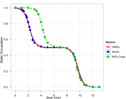
the differences were minimal. In Case Studies III and IV, I will give results that
show both minor and dramatic deviations.
A nice feature of stochastic simulations is that we are not confined by the same
limits as deterministic calculus-based models. We are not confined to talking about
the average evolution of populations, and we can explicitly treat non-ideal
interac-tions with reaction rate funcinterac-tions or “rules”. The implementation of such non-ideal
interactions was discussed by Pauling as early as 1935, but only explicitly
elabo-rated in statistical models by Chay in 1973.
Gillespie’s stochastic simulation algorithm (SSA) has become synonymous with
stochastic simulation of chemical reaction networks. Gillespie’s method is an
ex-act method, meaning that it represents the probabilistic distribution without
ap-proximation. Gillespie [1976] proposed a generalized algorithm that can be used
to reproduce the computational results of a deterministic model for well-mixed
chemical reactions using stochastic approaches. In order to evaluate the merits of
using the stochastic approach to quantitatively model cooperative chemical
sys-tems, we will use Gillespie’s SSA to fit observed experimental results, and then
compare these results to those obtained with a standard numerical integration of
the coupled ordinary differential equations that describe the details of the chemical
or biochemical reaction mechanism.
5.2.1
Gillespie’s Stochastic Simulation Algorithm
According to Gillespie’s SSA, reaction propensity functions are defined and
evaluated for each reaction under consideration. The reaction propensity provides
a measure of the likelihood that a chemical reaction or a single step in an overall
reaction mechanism will occur (i.e., high propensity is equivalent to a high reaction
probability). The reaction propensity functions are used to generate a
time-to-the-next-event function.
The reaction propensity is directly related to the probability that a specific
re-action or a single step in a rere-action mechanism will actually occur. The rere-action
propensity is formulated in terms of a reaction parameter which is analogous in its
general form to the corresponding reaction rate, a deterministic rate.
The intrinsic reversibility (e.g., a reversible chemical reaction that reaches true
equilibrium or reaches a steady-state condition such that∆G = 0,∆G◦= -RT(ln K),
and -d[A]/dt = -d[B]/dt = d[C]/dt) of the reaction of Equation 5.1 allows for the
reaction propensities of the forward and reserve steps to be written in a
straight-forward manner. For example, the reaction propensity for the straight-forward bimolecular
reaction between A and B is written as
propensity2 =kon(A×B) (5.6)
where kon is a second-order stochastic reaction parameter, A is the total number
of molecules of type Ain the reacting system during a single time-step iteration,
and B equals the total number of molecules of type B in the system during the
same iteration. Therefore, the productA ×B gives the total number of possible combinations of reaction events that can occur during a single time–step.
In the case of the reverse unimolecular reaction step, the corresponding reaction
propensity is given by:
propensity1 =kof f(C) (5.7)
wherekof f is a first-order stochastic reaction parameter andCis the total number
of molecules of typeC in the reacting system over a single iteration or time-step.
In order to determine an appropriate time-step, we take the sum of the reaction
propensities to generate total propensity (TP) as follows:
total propensity(T P) =X i
(reaction propensity). (5.8)
This total propensity is then used to generate an exponential random variable that
is equated to the time that the next individual molecular reaction will occur (τ).
The characteristic time-stepτ is thereby obtained from the following relationship:
τ =
1 (T P)ln
1 U RN
(5.9)
whereURNis a uniformly distributed random number between 0 and 1. It should
be noted that, as the total propensity of the system increases,τ decreases.
After the time-step τ is determined, the time to the next reaction event is
cho-sen. In turn, the reaction event that is to occur is chosen randomly with a bias
toward reactions with a greater propensity. Finally, the number of molecules are
updated appropriately to reflect the reaction that occurred.
Gillespie’s SSA approach [1976] was employed for the stochastic modeling
com-parison to the corresponding deterministic solutions. The SSA was implemented
in Scipy.
1. Computation is initiated at time t = 0 with the iteration number also set to zero.
2. The reaction propensities are calculated. 3. The appropriate time–stepτ is determined.
4. Given the computed reaction propensities, the specific reaction events during a single iteration are determined.
5. The current iteration is increased by 1 until an END value is reached at a maximum set time, or a limiting number of iterations is reached.
6. The total number of molecules in the reacting system is updated based upon the specific chemical reaction that is allowed to occur and the sequence is looped back to step 1 above.
Stochastic simulations were run to equilibrium for 200 repetitions and the data
was averaged. Sample codes are provided in the Appendix.
While the SSA was derived from statistical mechanics, lattice-like models were
not explored until approximately thirty years later in the form of rule-based
mod-eling.
5.2.2
Functional Elements of Macromolecules
Typical biochemists might have little intuition concerning the π−calculus or κ−calculus, referred to by Danos and colleagues [2004]. Furthermore, renaming molecules as agents is by no means required. It has been generally understood
since the early 19th century that macromolecules are composed of functional
ele-ments that affect the rates of reactions.
Again, the earliest application of a stochastic approach to model an autocatalyst
such as hemoglobin is attributed to Delbruck [1940]. Using Delbruck’s approach,
we normalize the molecular numbers to one Hb macromolecule. This is
analo-gous to constructing a finite element around a single molecule. Additionally, my
work is closely related to other rule-based modeling packages in that the most
fundamental algorithms should be similar. These similarities relate to the
realiza-tion that reacrealiza-tion rates are dynamic and that biochemical systems are non-ideal.
One important difference that we will highlight is that differential equations and
stochastic simulations predict different behavior for cooperative systems in small
volumes. Another difference in my approach is that we will provide source code
that others may run to gain insight into rate laws for non-ideal systems.
5.3
Additional Details
5.3.1
Hardware
Kinetic simulations were run on the following systems:
• A custom-built computer with the following specifications:
– Intel Quad Core Duo
– 8Gb of RAM
– Abit IP-35Pro motherboard
– running Ubuntu Linux
• An iMac running an intel core i5 processor
5.3.2
Software
Software codes written in Python Pyt23, Scipy, Matplotlib, and Pylab were used
for both deterministic and stochastic modeling.
5.3.3
Optimization
Code optimization was constrained by the data of Mills and Ackers et al. [1976]
using the Nedler-Mead method or the downhill simplex method . This algorithm
is contained in Scipy(Sci) in the function scipy.optomize.fmin.
5.3.4
Data Digitization
Four data-sets of Mills [1976] were digitized using the open source application
g3data.
5.3.5
Deterministic Methods
The corresponding systems of differential equations that correspond to the
de-tailed reaction mechanisms for two different experimental case studies were
nu-merically integrated using the variable-coefficient ordinary differential equation
solver, with a fixed-leading-coefficient implementation (VODE) . This method was
also implemented via Scipy through the integrate.ode method. Sample codes are
provided in the appendices. In some cases, Kinpy (Srinivasan) was used to
auto-generate complicated reaction schemes.