Robust Stabilization of Non-minimum Phase System with Periodic Control

(1)

International Journal of Emerging Technology and Advanced Engineering

Website: www.ijetae.com (ISSN 2250-2459,ISO 9001:2008 Certified Journal, Volume 5, Issue 4, April 2015)

252

Robust Stabilization of Non-minimum Phase System with

Periodic Control

Arindam Chakraborty

1

,

Jayati Dey

2

1, 2_{Department of Electrical Engineering, NIT Durgapur, Durgapur 713209, India}

Abstract— In the present work, implementation of continuous-time high frequency periodic controller is done for stabilization of non-minimum phase system having both right half plane (RHP) pole and zero. This work considers non-minimum phase cart-inverted pendulum system as a test bench. The robustness property of the periodic controller is compared with that of a linear quadratic regulator (LQR) and sliding mode control (SMC). The periodic controller is designed and shown to stabilize the cart-inverted pendulum system even in presence of plant parameter variations, external disturbances and measurement noise. Further, it is revealed that the periodic controller can cope up with the disturbance caused by rail inclination which is a common problem met by mobile robots while moving on an inclined plane.

Keywords—Cart-inverted pendulum, Non-minimum phase system, Periodic Controller, Robustness, Stabilization

I. INTRODUCTION

To ensure robust stability for non-minimum phase system having both RHP poles and zeros, is a challenging problem in control system. It becomes sometimes unachievable when the RHP poles and zeros are in close vicinity to each other. Linear time-invariant (LTI) controllers cannot provide robustness for such systems [1], [2]. This is due to the fact that the plant RHP zeros remain present in the loop transfer function which results in poor robustness margins. Further, additional poles and zeros appearing in loop transfer function due to pole-placement may render the closed-loop system response undesirable from robustness point of view.

On the contrary, some valuable results in literature show that time varying controllers can ensure robustness for non-minimum phase systems. Among them, the continuous-time high frequency periodic controllers presented in [3], [4] is capable to place the RHP zeros in the left half plane (LHP) leading to ―loop zero placement‖. This competence of the periodic controller, in turn, results in ensuring robustness of the compensated system leading to infinite gain margin (GM).

This paper employs the continuous-time high frequency periodic controller for robust stabilization of cart-inverted pendulum system in real-time. The cart-inverted pendulum is chosen since this system is a common example of non-minimum phase system. Linearization around the upright equilibrium point of the cart inverted pendulum system reveals that the system not only is unstable but non-minimum phase also, since it contains RHP zero. Moreover, the RHP poles and zeros are in close vicinity to each other.

Several control techniques involved in inverted pendulum system, ranging from simple conventional controllers to modern nonlinear control theory [5-12]. Among them the time variant controllers cannot achieve satisfactory loop robustness. In [13], the time varying periodic controller presented in [4] has been tested in real-time on cart-inverted pendulum system, and has been shown to achieve remarkably high GM. However the efficacy of periodic controller for phase margin and other robustness aspects even under plant uncertainties is not verified before.

(2)

International Journal of Emerging Technology and Advanced Engineering

253

 

1 1 m r m

A g BC BH

x x

G t L C g F t K C F t K

z        z

              _ _ _ _ _ _ _ _          

 

1 1 1 1 ( – ) m m r m m

q B g B

v d

Q q F  t K G   t L g F  t K 

        _ _ _ _  _  _   _  _    

,

 





 

0 x t

y t C d

z t

 

 _ _

 

(3)

 

  1 1 1 1 1 1 r r r r

n m n r

m

A BH _x

x

GC  F LC G CA b G H b  L F 

             __ _                      1 1 0

0 0 0

( ) ( )

r

m r F m

v v d d

Q G

Q   G  L    

        _                      

,

y t

 



C 0



x d

  

 _{ }

[image:2.612.65.550.559.725.2]

 

(4)

Fig. 1. The 2 DOF Periodic Controller [et. al. Das, Dey] In addition, this work attempts to verify the effectiveness

of the periodic controller on rejection of the disturbance caused by rail inclination. The problem of rail inclination is considered due to the fact that the two wheel mobile robots works in the principle of cart-inverted pendulum system. Considering the gravity of the pendulum according to the inclined angle, the dynamics of the system gets changed and the mobile robot motion is required to be controlled to keep the inverted pendulum upright while the mobile robot is changing the location.

II. BRIEF OVERVIEW OF PERIODIC CONTROL

Consider a SISO, LTI plant Gp

 

s B s₀( ) /A s₀( )of order n and relative order rwith

 

1

0 1 1 0

n n

n

A s s as a sa

 

1

0 1 0

n r n r n r n r

B s b_ s  b_ s  b s b ,

r



1

With its state space representation as

,

xAx Bu y Cx Du   (1)

Let us consider that the plant is compensated by a periodic controller of order m with unity feedback (Fig. 1) which is represented [4] as follows

 

m1



–



m1

z_F t K__z G _ y  Q _v_

_G  r

  

t L_ y 



Qv

uHz g _m_₁



y – 



q_m_₁v z , Rm , (2) W here y is the output of the plant including disturbance d, u is the output of the controller, v is the reference input,  is the noise,z denotes the controller

states, 1 ,0_   1 and 0m1 1 m1 m1

T I F F              , ( 1) [0_{m m} _m]

K _{ } k ,H[0_{1 (}__m_₁₎ 1], [ ₁ ₂ ]T m

G g g  g ,

1 2

[ 0 0]T

m r

L l l  l _  , [ ₁ ₂ ]T

m

F f f  f ,

1 2 [ m]T

Q q q q , ₁ [0₁_ ₁_ ₁]T

m m m

G _  _{ } g _ , ₁ [0₁_{ }₁ ₁]T

m m m

Q_  _{ } q _ ,

 

t cos( t)

 





,

 

 

t sin(



t)as is evenr and

 



t

 



t



cos as ris odd.

Combining (1) with (2) the closed loop system equations become (3) as shown at bottom of this page.

Now aassuming d, to be step or slowly varying (compared to) continuous periodic functions andv t( ) to be either (i) step whence it is additionally required that

1 0

m

q _  or (ii) slowly varying (compared to) continuous periodic function. Then, for any  0 and for allt0, there exists an ₀ such that for all   ₀the

(3)

International Journal of Emerging Technology and Advanced Engineering

[image:3.612.343.521.151.248.2]

254

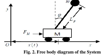
Fig. 2. Free body diagram of the System.

TABLE I

NOMINAL PLANT PARAMETERS

Parameter Symbol Value

Cart Mass M 2.4kg

Pendulum Mass _m 0.23kg

Pendulum Length Lp 0.36m

Acceleration due to gravity g 9.81_m _sec2

Pole Moment of inertia I 2

0.03kgm

Voltage to force factor _K

M 8N/V

where  1 ( 1)  1 1 1 ( 1)

0 Φ

0

T

m m m

m

I



      

 

  

 

 

and km dt

e 

   .

Since the amplitude of an ac signal ( sintorcost) passing through an integrator gets reduced by a factor equal to its frequency, it then follows from Fig. 1 that the choice of li 0, r2, ensures that the controller output contains oscillations of O(1) amplitude only. Obviously then the plant output would contain the periodic oscillations

of_O



1r



_.

The characteristic polynomial obtained from the averaged system (4) is

 

s A s F s0

   

Z s

 

   (5)

 

   





1

   

2

0 1 0

m

m n r

s B s G s g s b A

Z        s L s (6)

 

2 2

1

2 2 2 1

2 ... 1

m m

m

s f f s f f s

F         s    s (7)

 

2 2 2

1 2 1 2 ....

m m

s g g s g s

G        _   





1

r m m

m m r m

g l s g s

    

 



 

 (8)

   

( ) 1

1 2

1r r [ ... _{m r} m r ]

L s      l l s l _ s   (9) It is seen from (6) that Z s( ) is associated with the plant multiplication gain which is here considered to be of nominal value 1. When the multiplication gain tends to ∞, the closed poles terminate at loop zeros which are nothing

but the roots of the Z s( ). Hence Z s( )is known as loop zero polynomial. It now follows from (6) that the original plant zeros do not remain invariant and, in fact, the entire loop zeros can be placed arbitrarily (except when B s₀( )and

0( )

A s both have common RHP roots). This is referred to as "loop zero-placement". This allows one additional freedom

in the choices of Z s( ) polynomial so as to ensure that all the loop zeros are suitably placed in the left half plane (LHP). Now from (6) and (7), (8), and (9), 2m r 1 number of the controller parameters,g_i's andl_i's, assign the coefficients of



m n r 



th order loop zero polynomialZ s( ). Then one must have 2m r       1 m n r 1 m n. Therefore for loop zero and closed-loop pole placement, one may choosemn [4].

III. SYSTEM MODELLING

The Cart-inverted pendulum system made by ―FEEDBACK INSTRUMENTS LIMITED‖, UK, is used as the experimental. The cart-inverted pendulum system consists of a cart moving along a 1m rail. A driving mechanism with dc motor and belt-pulley transmission and an aluminum rod which is free to rotate about a pivot hinged to the cart. The back and forth movement of the cart caused by pulling the belt in two directions by applying voltage (2.5V) to the DC motor. By applying a voltage to the motor the force with which the cart is pulled, can be controlled.

Referring to Fig. 2 the mathematical model of the system is found by using Euler-Lagrange‘s equations as follows.

The kinetic energy (

K

_E) and potential energy (

P

_E) of the system are, respectively,



2 2 2



2 2

1 1 1

2 cos

2 2 2

E p p

K  m x  L x L   I  Mx (10)

cos

E p

P mgL . (11)

The symbols appearing in (10) and (11) are enlisted in Table I, along with their numerical values for the inverted pendulum system as described.

The Lagrangian of the entire system is

2 2 2 2 2

1 1 1

2 cos

2 mx mL xp mLp 2Mx 2I

   

_ _    _ _

 

     

L

cos p mgL

[image:3.612.327.563.552.716.2]

(4)

International Journal of Emerging Technology and Advanced Engineering

[image:4.612.48.285.530.689.2]

255

Fig. 3. Stabilizing Control Scheme The Euler-Lagrange‘s equation for the cart and the

resultant system is given by

( ) _M

d

bx F dt x  x 

 

L L

(13)

( ) 0

d

dt   

  _

 

L L

(14)

From (13)-(14), the non-linear mathematical model of the cart and pendulum system is obtained, and is given by (15) and (16)





2 1

[ _p sin cos ]

p

mL g x d

I mL

  



    , (15)



2



1

[ _M _p cos sin ]

x F mL bx

M m

   

     . (16)

The mathematical model described in (15) and (16) are used to model the open-loop inverted pendulum whereas the same non-linear model is used for the design of the swing-up controller. The inverted position of the pendulum corresponds to the unstable equilibrium point



 ,

  

 0, 0 . After linearization one obtains,



2



p p p

ImL mgL mL x d  , (17)



Mm x bx mL



  pFM . (18)

The control input uF_M K_M is the motor voltage to be applied, wherekis the motor voltage to force factor considered. From (17) and (18) the state-space form of the system can be found with negligible frictions

M

XAXBF , yCX (19)









2

0 1 0 0

( )

0 0 0

0 0 0 1

( )

0 0 0

p p

c p c p p

c p p p

L m g

I M m M m L A

M m L m g

I M m Mm L

   _     _ _             _ _    ,









2 2 2 0 ( 0 ) p p

c p c p p

p p

c p c p p

I m L

I M m M m L

B

L m

I M m M m L

                           ,

1 0 0 0

0 0 1 0

C  _

 , the state vector





T

X x x  

and the output vectory



x 



T.

Substituting the numerical values in (19), one obtains

0 1 0 0

0 0 0.0199 0.4471 0.0028

0.3976

0 0 0 1 ,

0 0 0.0275 14.2002 0.0874

0.5504 A B      _ _               _      _      

. (20)

IV. STABILIZATION WITH PERIODIC CONTROLLER

[image:4.612.344.560.619.711.2]

The system described by (20) has been remodeled as in Fig. 3 where u to cause  and  in turn cause to x and the corresponding transfer functions are given below







2

0.3976 3.6853 3.6853 ( )

( ) 0.5504

s s

x s

s s

  



 , (21)







( ) 0.5504

( ) 3.7683 3.7683

M

s

F s s s

 

 



. (22)

It is clear from (21) and (22) that x s( ) /F_M

 

s has a close proximity of RHP pole (at 3.7683) and zero (at 3.6853). The inner loop gains used in design are

1 95.74

K   andK₂ 307.62. The resulting compensated transfer function for inner and outer loop becomes

 

  

49.560.5504



3.13



M

s

F s s s

 

 



, (23)











2

0.3976 3.6853 ( 3.6853) ( )

( ) 49.56 3.13

M

s s

x s

F s s s s

 



  . (24)

The periodic controller design for G s_p( )x s( ) /F_M

 

s

is based directly on the design procedure discussed in Section II. Here m n 4 and r2.

In order to relocate the loop zeros in the LHP for satisfactory loop robustness and for an acceptable response

(5)

International Journal of Emerging Technology and Advanced Engineering

256

  

s s 49.56



s 1 j



s 0.5



     



s 5.63 2j



s 3.6853 (



s 1.85)

     , (25)

  







2

3.6853 ( 3.5) 4.5

s s s

F    s . (26)

This choice has been done allowing maximum number of LHP pole-zero cancellation. The resulting loop zero polynomial is found, following (5), to be

  

49.56



3.6853



2.0869



Z s  s s s



s 0.3201 (



s 2.8813 3.5572 )j

    . (27)

The controller parameters hence are obtained by

equating the coefficients of _sk_,

k0 to 6 for Z s( ) given in (6) and (27) with (7), (8) and (9), as

1 1397.7, 2 5796.2, 3 1643.8, 4 160.5 , 5 2.6,

g  g  g  g  g  

1 533.0289, 2 144.6365,3 4 0,

l  l  l  l f₁ 162.9496,

2 163.1952, 3 61.0237,

f   f   f₄ 16.1853 with

1 2 3 0, 4 1

k k k  k  and 1 .2661.

V. IMPLEMENTATION OF PERIODIC CONTROLLER

The inverted pendulum system used here is associated with upper limit of the sampling rate be 333Hz depending upon the sensor and ADC resolution, whereas the speed of response of the system determines the lower limit to be 25Hz. The periodic controller designed above is implemented on the cart-pendulum system described in Section III, for the controller frequency,₀25Hz.

A. Robustness with gain margin

A measure of closed-loop robustness

is  _ sup_

 

jω _, where 

 

jω is the sensitivity transfer function. For a satisfactory result, _ is required to be



2

which simultaneously satisfies GM



2

and phase margin 0

30

[image:5.612.326.562.136.307.2]

 [1-2]. The sensitivity transfer function for cart-inverted pendulum system compensated with the periodic controller designed in Section IV is found as

Fig. 4. The Sensitivity Characteristics.

 

_

2



_

3.13 (



_

3.5)



4.5

_



2

1 0.5 5.63 2 ( 1.85)

s s s s

s j s s j s

s   

 

      . (28)

The sensitivity characteristic (Fig.4) shows that 1.57



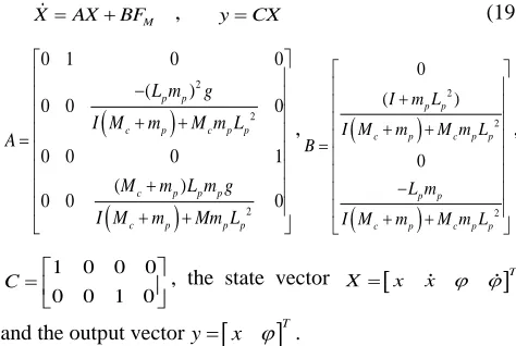
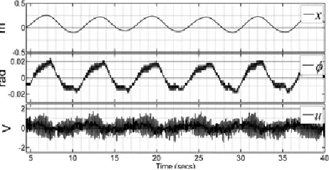
  which signifies a satisfactory robust design. The robustness of the physical cart–pendulum system compensated using the periodic controller is studied with respect to the variations of the multiplicative gain (G) in the outer loop shown in Fig.3. The , ,x u plots for nominal and other two extreme gains are shown in Figs. 5-7. The ratio of the maximum (4.31) and minimum (0.38) gain for which the pendulum remains upright under system tolerances is 11.34.

Comparison with LQR

The state feedback controller is designed based on the linear quadratic regulator principle for the linear model of the system (20).

[image:5.612.328.559.494.614.2]

(6)

International Journal of Emerging Technology and Advanced Engineering

[image:6.612.54.285.120.412.2]

257 Fig. 6. Periodic control with gain = 0.38

Fig. 7. Periodic control with gain = 4.31

Here for the systemX t

 

AX t

 

Bu t

 

, the control law is given by u t

 

 KX

 

t .The matrix gain K has been determined such that the static, full-state feedback control lawu t( )minimizes the quadratic functional

 

   

0

T T

J K X t QX t u t Ru t dt



 





_  _ , with Q is a

nonnegative-definite matrix that penalizes the departure of system states from the equilibrium and R is a positive-definite matrix that penalizes the control input. An acceptable values to achieve small settling time under physical system restriction ( 2.5 V  u 2.5V), are

found to be Qdiag 3000;0;9;0





andR1500. The

closed loop poles are placed

[image:6.612.326.562.133.535.2]

at3.7540, 3.7723, 1.3745 1.3589   j. The dominant closed loop poles with damping factor, 0.71s and natural frequency, 1.93 rad/s, resulting in a settling time of approximately 3s. With these design parameters, the feedback gains are obtained as K= [-1.22 -3.19 -66.55 -17.75].

Fig. 8. LQR with nominal gain

Fig. 9. LQR with gain=0.54

Fig. 10. LQR with gain=1.42

This controller has been implemented on real time with the system discussed in Section III. It has been observed that the ratio of maximum (1.42) and minimum (0.54) gain for which the pendulum remains upright and within system tolerance is 2.63. The , ,x u plots for nominal and other two extreme gains are shown in Figs. 8-10.

Comparison with SMC

(7)

International Journal of Emerging Technology and Advanced Engineering

258 SMC design can be divided into two subparts: (i) design of a stable switching surface (sliding surface, [12]) and (ii) design of a control law to force the system states onto the chosen surface in finite time. The sliding surface equation is obtained following [14], as _{S x}( )_{G X}T _where

( )

T T

G e P A , discussed later. The control law must be

designed such that the reaching condition S S0 is satisfied. This criterion should be fulfilled to ensure that the state will move toward and reach the chosen sliding surface. The control law that will be implemented into this sliding mode control structure is presented asu M sgn S X( ( )), where M is the design parameter and

1, 0

sgn( ) 0, 0

1, 0

S

S S

S

  

 

 



The value of G can be obtained by using Ackermann formula [15], as follows





₂ ₃ 1

0 0 0 1 * * * *

T

e  _B A B A B A B_ . Now, if the desired eigen values are   i,i n 1, n is the

order of the plant, then

  

1



2



3



P A  AI AI AI , where I is the identity matrix of same order as A. Choosing the eigen values as-1, -2,-3 one can find

[ 1.113 2.0373 11.7041 3.2885]

T

G     

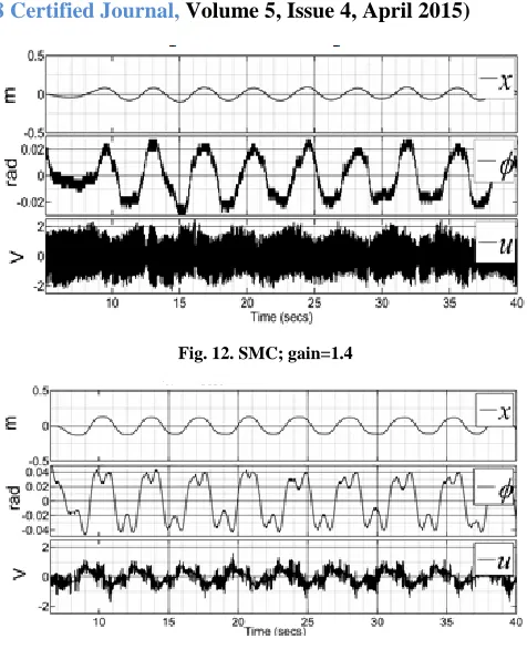
[image:7.612.324.562.120.413.2]

The value of M is figured out by debugging the MATLAB model of the inverted pendulum using trial and error method. Being the design parameter it is chosen as 10. The response for nominal and other two extreme gains are shown in Figs. 11-13. The GM of the SMC is found to be 5.38.

Fig.11. SMC nominal gain

Fig. 12. SMC; gain=1.4

Fig. 13. SMC; gain=0.26

B. Delay Margin

The maximum delay, _d is the largest of  , beyond

which the system

 

sd

p

G s e becomes unstable. Hence the system (with phase margin, PM, and corresponding gain crossover frequency,



) on the verge of instability, may be represented as _{G j}

 

 _ejd  1_{. By equating angles,} one can find





0

0 0

180

180 180

d

G j  PM 



 

 

   

With the periodic controller designed and synthesized above, the system PM and  are obtained as 45.4 and 0 0.977 rad/sec. Therefore theoretically maximum delay is

0.81

d 

[image:7.612.50.284.574.697.2]

(8)

International Journal of Emerging Technology and Advanced Engineering

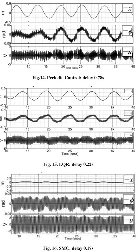
[image:8.612.50.287.137.572.2]

259 Fig.14. Periodic Control: delay 0.78s

Fig. 15. LQR: delay 0.22s

Fig. 16. SMC: delay 0.17s

On the other hand, the delay margin for LQR and SMC is found out to be 0.22s and 0.17s (Figs. 15-16).

C. Noise Attenuation

In the present work, a sinusoid of amplitude 0.05m and frequency of 83Hz is being synthetically added to the cart position at 20s and withdrawn at 41.5s. This acts as a measurement noise. It is shown in Fig.17a that although, due to the applied noise, the deviation of angle has increased by 0.0131 rad compared with the nominal; the periodic controller is successfully stabilizing the system in presence of this noise.

It is interesting to note from Fig.17a shows that in presence of the noise, the steady state value of the position and angle do not have any effect at all. This means the noise is completely attenuated by the periodic controller. This result is justified as follows.

[image:8.612.327.561.227.352.2]

The frequency response of the noise to output transfer function,

Fig. 17a. Frequency response of noise to output transfer function

Fig. 17b. Noise Attenuation

   

0

   





1

 

2

[ 1 m]

m

Y s N s B s G s   g _s  s for the designed periodic controller in the Section IV is

shown in Fig. 17b. It is observed that Y

   

j N j vs ω

characteristic attains a value of approximately at the frequency 83Hz. This signifies that the periodic controller can attenuate a noise signal of frequency 83Hz by a factor

4

10 5  .

D. Disturbance Rejection

The disturbance to output transfer function,

   

 

_{ }





1 1

2

0 [ 1 ]

m m

n r n

A s F s b L s b g Y s D

s

s   s

 

   



(9)

International Journal of Emerging Technology and Advanced Engineering

260 It is seen from the figure that the Y

   

j D j vs ω

characteristic is having a slope of -40db/decade approximately. Hence, it is expected that a step disturbance having frequency near to zero will be greatly attenuated by the periodic controller.

This theoretical anticipation is verified with the following experimentation. The external disturbances are applied on  which cause the angle deviation of 0.0157

[image:9.612.54.283.282.419.2]

rad from the nominal in both directions at 33.3s and 50.5s. At 67.8s, a disturbance for an angle deviation of 0.0209 rad from the nominal is applied.

[image:9.612.325.557.289.469.2]

Fig. 18a. Frequency response of disturbance to output transfer function

Fig. 18b. Disturbance rejection in real-time

This is the maximum disturbance that can be applied in this system as the cart position reaches at 0.5m and the control voltage to -2.5V. The controller rejects these disturbances in 7.3s for formers and 8.2s for the next. A disturbance torque is applied on the pendulum by sudden ‗pushes‘ of very short time duration. Fig.18b shows disturbance rejection property of periodic controller in real time where disturbances are applied on upright stabilized pendulum, at three different instants of time in the opposite direction of the cart movement.

E. Plant Parameter Variation

The plant parameters such as pendulum length (L), pendulum mass (m) and cart mass (M) has been changed and the robustness properties of the periodic controller designed has been examined in real time under these plant parameters variation and observed to stabilize the pendulum at its upright equilibrium point within rail limit.

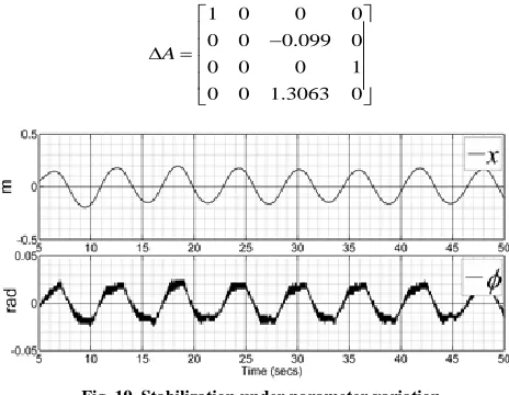
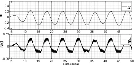
The simultaneous plant parameter additive perturbation of 21% for cart and pendulum mass and 11% for pendulum length is introduced as follows:M_u M_M,m_u  m _m,

u L

L  L  with the entire time frame. This perturbation introduces uncertainty in the system matrix as

1 0 0 0

0 0 0.099 0

0 0 0 1

0 0 1.3063 0

A

 

 _ 

 

 _ _

 

 

Fig. 19. Stabilization under parametervariation

In presence of these uncertainties, it is observed via Fig. 19 that both controllers are capable of stabilizing the system.

F. Rail inclination

Inclination of the rail is the greatest source of disturbance that occurs when controlling the inverted pendulum attached with the cart.

The angle of the inclination of the rail if changed from vertical surface of earth (_{0 ) to some angle (}0 _{), the} central angle of the inverted pendulum gets changed which actually causes the model uncertainty. Fig.20 shows that the periodic controller can cope up with such uncertainties for inclination angle,30.

VI. CONCLUSION

[image:9.612.50.288.442.576.2]

(10)

International Journal of Emerging Technology and Advanced Engineering

[image:10.612.50.285.388.502.2]

261 The performance comparison has been done with LQR and SMC. The veracity of the claim has been established through experimental results. The continuous-time periodic controller has provided superior gain (11.34, w.r.t 2.63 for LQR and 5.38 for SMC) and delay margin (0.78s, w.r.t 0.22s for LQR and 0.17s for SMC) to a non-minimum phase cart-inverted pendulum system by virtue of its loop zero-placement capability. It has been shown in real-time that the periodic controller can achieve robust stabilization even under plant parameter variation. The disturbance rejection and noise attenuation capabilities of the periodic controller have also been verified through experimentation. Further, the cart-inverted pendulum has been shown to be stabilized with the periodic controller even when the rail is inclined. This, in turn, implies that the periodic controller can stabilize a mobile robot while moving on an inclined plane. The results presented in this paper also prove the claim made in literature that a time-varying controller can achieve what a linear time-invariant controller does in the direction of disturbance rejection and noise attenuation [16], [17].

Fig. 20. Robust Stabilization with rail inclination

REFERENCES

[1] Doyle, J. C., Francis B. A. and Tannenbaum, A. R. 1992 Feedback Control Theory. New York: Macmillan Publishing Company. [2] Wolovich, W. A. 1994 Automatic Control Systems. Rochester, NY:

Saunders College Publishing.

[3] Lee, S., Meerkov, S. M. and Runolfsson, T. 1987. Vibrational feedback control: zeros placement capabilities. IEEE Trans. on Automatic Control, vol. 32, no.7, 604–611.

[4] Das, Sarit K. and Dey, J. 2007. Periodic compensation of continuous-time plants. IEEE Transactions on Automatic Control, vol. 52, no. 5, 898–904.

[5] Omatu. S. and Yashioka, M. 1998. Stability of inverted pendulum by neuro-pid control with genetic algorithm. In Proceedings of the IEEE International Joint Conference on Neural Networks. 2142-2145. [6] Ghosh, A., Krishnan, T. R. and Subudhi, B. 2011. Robust

proportional-integral-derivative compensation of an inverted cart-pendulum system: an experimental study. IET Con. Th. and App., vol. 6, no. 8, 1145-1152.

[7] Magaña, M. E. and Holzapfel, F. 1998. Fuzzy Logic Control of an Inverted Pendulum with Vision Feedback. IEEE Trans. on Education, vol. 41, No. 2,165-170.

[8] Anderson, C. 1989. Learning to control an inverted pendulum using neural networks. IEEE Control Sys. Magazine, vol. 9, no. 3, 31-36. [9] Ghanbarie A. and Farrokhi, M. 2006. Decentralized decoupled

sliding-mode control for two-dimensional inverted pendulum using neuro-fuzzy modeling. In Proceedings of IEEE International Conference on Engineering of Intelligent Systems, 1-6.

[10] Edwards, C. and Spurgeon, S. K. 1998. Sliding Mode Control: Theory and Applications, Abingdon, UK: Taylor and Francis. [11] Seshagiri, S. and Khalil, H. K. 2002. On Introducing Integral Action

in Sliding Mode Control. In Proceedings of 41st IEEE Conference on Decision and Control, 1473-1476.

[12] De Carlo, R.A., Zak, S.H. and Matthews, G.P. 1988.Variable Structure Control of Nonlinear Multivariable systems: A Tutorial. In Proceedings of IEEE, vol.76, no.3, 212-232.

[13] Das S. K. and Paul, K. K. 2011. Robust compensation of a Cart– Inverted Pendulum system using a periodic controller: Experimental results. Automatica, vol. 47, no. 11, 2543-2547.

[14] Utkin V, Guldner J, Shi J. 1999. Sliding Mode Control in Electromechanical Systems. UK: Taylor and Francis Ltd.

[15] Ackermann J, Utkin V. 1998. Sliding Mode Control Design Based on Ackermann‘s Formula. IEEE T Automatic Control, vol 43, no. 2, 234-237.

[16] Shamma J. S. and Dahleh, M. A. 1991. Time-varying versus time-invariant compensation for rejection of persistent bounded disturbances and robust stabilization. IEEE Transactions on Automatic Control, vol. 36, no.7, 838–847.