Document Clustering For Improving Computer Inspection

(1)

International Journal of Emerging Technology and Advanced Engineering

Website: www.ijetae.com (ISSN 2250-2459,ISO 9001:2008 Certified Journal, Volume 5, Issue 7, July 2015)

316

Document Clustering For Improving Computer Inspection

M. Shanthi

1

, Dr. K. Venkata Rao

2

1

M.Tech (C.S.T)2nd Year, Department of Computer Science & Systems Engineering, Andhra University, India

2_{Associate Professor, Department of Computer Science & Systems Engineering, Andhra University, India}

Abstract—Clustering is an approach that organizes a large quantity of unstructured text documents into a small number of meaningful and coherent clusters. Related to document clustering, clustering methods can be used to automatically group the retrieved documents into a list of useful categories. Document clustering has shown to be very useful for computer inspection. Numbers of files are examined in computer analysis. For computer examiners, it’s quite difficult to analyze the huge amount of data that was gathered from a computer system. In this context, automated methods of analysis are of great interest. In particular, algorithms for clustering documents can facilitate the discovery of new and useful knowledge from the documents under analysis.

There went a lot of research already and in this paper, we have experimented six known algorithms and presented their comparision.

Keywords— Clustering, Cosine Similarity, Data mining,

Text mining.

I. INTRODUCTION

A recent study reveals that the digital world as on today has its volume of data increased exponentially [1]. This shows how fast the data is growing.

This Computer Inspection involves examining large number of files obtained by each computer which will be the worst nightmare. Therefore, methods for automated data analysis, widely used for machine learning and data mining are significant. Algorithms for recognition of patterns from the information present in text documents are useful. Clustering is used when little knowledge about data is present [2], [3]. It focuses on clustering the text documents [7], [9] using various clustering algorithms [4]. The aim is to reduce the efforts of reading each and every document to assure its originality or relativity when a large set of documents are to be inspected.

Here, we employed many clustering algorithms and each algorithm has a different set of pros and cons. The rationale behind clustering algorithms is that objects within a valid cluster are more similar to each other than they are to objects belonging to a different cluster [2], [3]. Thus, once a data partition has been induced from data, the expert examiner might initially focus on reviewing representative documents from the obtained set of clusters. Then, after this preliminary analysis, (s) he may eventually decide to scrutinize other documents from each cluster.

By doing so, one can avoid the hard task of examining all the documents (individually) but, even if so desired, it still could be done.

As choosing a better clustering algorithm is a must in employing the algorithm for document clustering, we present a comparative study of the below six algorithms.

1. K-Means

2. Bisecting K-Means 3. Single Link 4. Complete Link 5. Average Link and 6. CSPA

As distance measure plays a major role in any clustering technique and that the document clustering involves measuring distance between terms, we choose cosine similarity measure.

The rest of the paper is so organized that the section 2 puts light on the algorithms and the distance measure and section 3 exhibits the experimental results, and then conclusion.

II. CLUSTERING ALGORITHMS AND COSINE DISTANCE MEASURE

Measuring distance between two clusters or between elements or element to a cluster is a primary job in clustering. As we speak about document clustering, which involves text data rather than numerical data, we have to employ cosine similarity measure. So first let us have a look into cosine similarity distance measure and then the algorithms.

A. Cosine Similarity Distance Measure

We simplify a document to a bag of words, in the following way called terms.

t Any single term d Any single document M Number of documents m Number of terms T {t1, . . . tm} C {d1, . . . dM}.

(2)

International Journal of Emerging Technology and Advanced Engineering

317

N(d) = Number of total terms occurrences in d

= ∑t n(d,t)

Q(d,t) = Natural probability distribution on CxT = n(d,t)/N

Q(d) = Natural probability distribution on C = N(d) / N

q(t) = Natural probability distribution on T = n(t)/n

And from these we derive the below conditional probabilities

And from these equations the distance measure between two terms t & s is derived as the below.

B. Data Pre-processing

Before the documents are clustered, a bag of words has to be extracted from each document. This is a step by step process

1.First all stop-words have to be removed, the current experiment is carried on English language hence, the parts of speech helps us identifying the stop words. In this experiment Articles, Adverbs, Aux Verbs, Prepositions, Conjunctions, Symbols, Punctuations, Interjunctions are all considered as stop words and are removed.

2.Now the root words are supposed to be identified and the word phrases shall be condensed to form the root that increases the word occurrence calculation properly and thus effecting the probabilities and thus enhance the distance measure. For this we have implemented the Lookup version of Stemming Algorithm.

C. Clustering Algorithms

The clustering algorithms used in our study the K-means [3] and Bisecting K-means the hierarchical Single/Complete/Average Link [5],[8] and the cluster ensemble based algorithm known as CSPA [6] are famous in the machine learning and data mining fields, and therefore they have been used in our study.

Unlike the partitional algorithm such as K-means, hierarchical algorithms such as Single/ Complete/Average Link provide a hierarchical set of nested partitions [3], usually represented in the form of a dendrogram, from which the best number of clusters can be estimated. In particular, one can assess the quality of every partition represented by the dendrogram, subsequently choosing the one that provides the best results [14]. The CSPA algorithm [6] essentially finds a consensus clustering from a cluster ensemble formed by a set of different data partitions.

K-Means:

K-Means is one of the simplest unsupervised learning algorithms that solve the well-known clustering problem. The procedure follows a simple and easy way to classify a given data set through a certain number of clusters (assume k clusters). The main idea is to define k centroids, one for each cluster. These centroids should be placed in a cunning way because of different location causes different result. So, the better choice is to place them as much as possible far away from each other. The next step is to take each point belonging to a given data set and associate it to the nearest centroid. When no point is pending, the first step is completed and an early group age is done. At this point we need to re-calculate k new centroids. After we have these k new centroids, a new binding has to be done between the same data set points and the nearest new centroid.

The algorithm is composed of following steps 1. Determine k

2. Choose k random terms as centroids

3. Pickup each term and compute distance matrix with the centroids and combine this term with the one that have the minimum distance

4. Recompute centroids

5. Repeat 3 and 4 until a consistent centroid set is formed.

(3)

International Journal of Emerging Technology and Advanced Engineering

318

Bisecting K-Means:

In bisecting k-means the entire dataset is bisected in such a way that the elements which are closer to centroid in one cluster and the remaining in other cluster. Now each cluster is bisected again as said above.

Fig2: Example of Bisecting K-Means

The algorithm is composed of following steps

1. Determine k

2. The entire term bag is considered a single cluster and its centroid is computed

3. The average distance between the min and max distance of each term to the centroid is computed.

4. The main cluster is bisected in such a way that the closest terms to the centroid are of one cluster and the farthest of the other cluster. Closest being the distance to the term and the centred is less than the computed average distance.

5. Repeat 3 and 4 until k or more clusters are formed.

Single Link:

Single Link is also called the K- Nearest Neighbourhood algorithm. Here, in each step we merge the two clusters whose two closest members have the minimum distance.

Fig3: Single Linkage

The algorithm is composed of following steps 1. Determine k

2. Each term is considered to be a single cluster

3. Compute distance matrix from one cluster to the other.

4. Combine two closest clusters (clusters with minimum distance between one another)

6. Repeat 3, 4 and 5 until k clusters are formed

Complete Link:

Complete Link is also called the K- Furthest Neighbourhood algorithm. Here, the clusters having maximum distance are merged.

1. Determine k

4. Combine two farthest clusters (clusters with maximum distance between one another)

6. Repeat 3, 4 and 5 until k clusters are formed.

Average Link:

Here, the clusters with average distance are merged.

1. Determine k

4. Combine two considerably closest clusters (clusters with distance between one another less than the average distance computed from the matrix)

6. Repeat 3,4 and 5 until k clusters are formed

CSPA:

If two objects are in the same cluster then they are considered to be fully similar, and if not they are dissimilar. This is the simplest heuristic and is used in the CSPA.

1. Determine a threshold th

2. Choose k random terms as centroids

3. Pickup each term and combine this term with the one centroid that has the distance below the th.

(4)

International Journal of Emerging Technology and Advanced Engineering

319

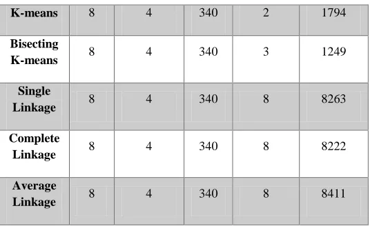
III. EXPERIMENTAL OBSERVATIONS

We have to consider a sample of text documents and the input k is given for each clustering algorithm. Then the resultant cluster counts and execution times have to be recorded.

From table I, it is shown that with a slow range of increase in the number of clusters, the time to form the clusters also increases. The Bisecting K-Means clustering algorithm has the shortest time to form the resultant clusters but the K-Means clustering algorithm results in better clusters with considerable speed which is less than the other clustering algorithms. Single Link, Complete Link and Average Link algorithms has nearly same execution times.

The below are our observations on a sample of documents collected.

TABLE I

Algorithm Input

k

Document Count

Term Count

Resultant Cluster

Count

Execution Time

(ms)

K-means 4 4 340 2 1326

Bisecting

K-means 4 4 340 3 1059

Single

Linkage 4 4 340 4 8385

Complete

Linkage 4 4 340 4 8224

Average

Linkage 4 4 340 4 8511

K-means 6 4 340 2 1538

Bisecting

K-means 6 4 340 4 1059

Single

Linkage 6 4 340 6 8272

Complete

Linkage 6 4 340 6 8181

Average

Linkage 6 4 340 6 8469

K-means 8 4 340 2 1794

Bisecting

K-means 8 4 340 3 1249

Single

Linkage 8 4 340 8 8263

Complete

Linkage 8 4 340 8 8222

Average

Linkage 8 4 340 8 8411

The following graphs are devised based on the recorded observations.

[image:4.612.311.579.131.295.2]

Fig4: Graph representing Execution Times

Fig 5: Graph representing the requested and resultant clusters 0

2000 4000 6000 8000 10000

2 4 6 8

T

im

e(

m

s)

Number of clusters

K-Means Bisecting K-Means Single Link Complete Link Average Link

0 2 4 6 8

K-Means Bisecting K-Means Single Link Complete Link Average Link K-Means Bisecting K-Means Single Link Complete Link Average Link

Cluster Formation

(5)

International Journal of Emerging Technology and Advanced Engineering

320

IV. CONCLUSION

Clustering has number of applications in every field of our life. We are applying this technique knowingly or unknowingly in our day-to-day life. One has to cluster a lot of things on the basis of similarity either consciously or unconsciously. It is very much evident from the experimental results that amongst the six algorithms, K-Means, Bisecting K-K-Means, Single Link, Complete Link, Average Link and CSPA, though the Bisecting K-Means and CSPA takes less time to form estimated clusters, the K-Means is performing considerable faster and results better clusters. Labelling is also done here so that it will be easy to search for a required document by just checking the label of that particular cluster. Hence, we can use document clustering on a large dataset of research papers as input and reduce the efforts of reading each and every document for analysis which would be beneficial for an organization working in relevance of research papers.

REFERENCES

[1] J. F. Gantz, D. Reinsel, C. Chute, W. Schlichting, J. McArthur, S.Minton, I. Xheneti, A. Toncheva, and A. Manfrediz, “The expanding digital universe: A forecast of worldwide information growth through 2010,” Inf. Data, vol. 1, pp. 1–21, 2007.

[2] B. S. Everitt, S. Landau, and M. Leese, Cluster Analysis. London, U.K.: Arnold, 2001.

[3] A. K. Jain and R. C. Dubes, Algorithms for Clustering Data. Engle- wood Cliffs, NJ: Prentice-Hall, 1988.

[4] M. Steinbach, G. Karypis, and V. Kumar. A comparison of document clustering techniques. In Proceedings of Workshop on Text Mining, 6th ACM SIGKDD International Conference on Data Mining (KDD’00), pages 109–110, August 20–23 2000.

[5] R. Xu and D. C.Wunsch, II, Clustering. Hoboken, NJ: Wiley/IEEE Press, 2009.

[6] A. Strehl and J. Ghosh, “Cluster ensembles: A knowledge reuse framework for combining multiple partitions,” J. Mach. Learning Res., vol. 3, pp. 583–617, 2002.

[7] S. Meyer zu Eissen and B. Stein. Analysis of clustering algorithms for web-based search. In D. Karagiannis and U. Reimer, editors, PAKM, volume 2569 of Lecture Notes in Computer Science, pages 168–178. Springer, 2002.

[8] Y. Zhao, G. Karypis, and U. M. Fayyad, “Hierarchical clustering algorithms for document datasets,” Data Min. Knowl. Discov., vol. 10, no.2, pp. 141–168, 2005.