Munich Personal RePEc Archive
Preference reversals in contingent and
inferred valuation methods
Stachtiaris, Spiros and Drichoutis, Andreas and Klonaris,
Stathis
Agricultural University of Athens, University of Ioannina
March 2011
Online at
https://mpra.ub.uni-muenchen.de/32800/
1
Preference reversals in Contingent and Inferred valuation
methods
Spiros Stachtiaris1, Andreas C. Drichoutis 2, Stathis Klonaris3
1
Department of Agricultural Economics & Rural Development, Agricultural University of
Athens, Iera Odos 75, 11855, Athens, Greece, email: [email protected]
2
Department of Economics, University of Ioannina, University Campus, 45110, Ioannina
Greece, email: [email protected]
3
Department of Agricultural Economics & Rural Development, Agricultural University of
Athens, Iera Odos 75, 11855, Athens, Greece, email: [email protected]
Abstract
We examine inconsistencies in preference orderings (Alevy et al. 2011) using the Contingent
valuation (CV) as well as the Inferred valuation (IV) method (Lusk and Norwood 2009a,b).
We find that when moving in the context of a food market we only observe weak effects of
inconsistencies. In addition, we find that the IV method is more susceptible to inconsistent
preference orderings than the CV method. We also find that the IV method generates higher
valuations than CV in case of consumers with high commitment costs but successfully
mitigates social desirability bias in case of low commitment costs and high normative
motivations.
Key words: willingness-to-pay (WTP),Contingent Valuation (CV), Inferred Valuation(IV),
preference reversals
2
Preference reversals in Contingent and Inferred valuation
methods
Abstract
We examine inconsistencies in preference orderings (Alevy et al. 2011) using the Contingent valuation (CV) as well as the Inferred valuation (IV) method (Lusk and Norwood 2009a,b). We find that when moving in the context of a food market we only observe weak effects of inconsistencies. In addition, we find that the IV method is more susceptible to inconsistent preference orderings than the CV method. We also find that the IV method generates higher valuations than CV in case of consumers with high commitment costs but successfully mitigates social desirability bias in case of low commitment costs and high normative motivations.
Key words: willingness-to-pay (WTP),Contingent Valuation (CV), Inferred Valuation(IV),
preference reversals
JEL codes: C9, C93, D12, Q51
I. Introduction
Eliciting people’s valuation for non-market goods has been central in the economics
literature. The Contingent Valuation method (CV) is by far the most popular valuation
method and a big bulk of the literature deals with refinements that (attempt to) address a
number of documented biases. Recently, Lusk and Norwood (2009a,b) developed a new
method for addressing the so-called social desirability bias, that is, the utility that people
derive from stating a value to please the researcher or themselves. Respondents, in the
presence of an interviewer may report socially desirable preferences, and thus misrepresent
their “true” preferences, in order to either please the interviewer or to be consistent with
social norms (Crowne and Marlowe 1960;Fisher 1993;Leggett et al. 2003;List et al.
3
acceptable" rather than speak his/her true feelings. Social desirability bias is intrinsic in CV
studies.
Lusk and Norwood (2009a) thought that instead of asking people what they are willing
to pay, to ask them what they think another (average) person would pay1. This form of
indirect questioning has been first proposed by Fisher (1993) which found that indirect
questioning affected responses in questions with normative context but not in questions with
personal motivation. This simple twist in the wording of the valuation question in Lusk and
Norwood (2009b) generated (inferred) valuations that were close to real valuations (as
compared to an experiment) and lower than hypothetical valuations (where social desirability
is prevalent). Their results were also confirmed in Lusk and Norwood (2009a) but in this
study the emphasis was put in exploring the role of normative motivations and the gap
between the lab and the field. The authors showed that goods with normative dimensions are
more prone to social desirability bias and thus the inferred valuation method is more effective
in bridging the gap between the lab and the field valuations. The role of familiarity with the
product and commitment costs were central in the analysis as well, since they found that
people overstated their preferences for relatively familiar goods with normative attributes and
understated their preferences for unfamiliar goods with low normative motivations.
Lusk and Norwood (2009a,b) coined the term Inferred Valuation (IV) to describe this
type of indirect questioning in valuation studies. The aim of the IV method is not only to
alleviate social desirability but also to moderate hypothetical bias. With the CV method
people uncover preferences possibly including normative or moral considerations. On the
contrary, with the IV method individuals are asked to predict how other people would behave
and thus infer other’s people preferences that are ideally free from normative or moral
1
4
considerations. A natural question that follows is whether this prediction of preferences could
result in more consistent and well defined preference orderings as compared to standard
preference elicitation methods such as CV.
The often cited strand of the literature that deals with non-consistent preference
orderings is the preference reversal literature (see Seidl 2002 for a review). Broadly defined,
any systematic change in preference orderings between normatively equivalent conditions
can be called a preference-reversal (Slovic and Lichtenstein 1983). The preference reversals
literature took off with the study of Slovic and Lichtenstein (1968) and the help of
economists (Grether and Plott 1979) that demonstrated the robustness of the effect. The
phenomenon is an empirical regularity such that a pricing task for lotteries reveals opposite
preferences from a choice task made out of the lotteries.
More recently, List (2002) (as well as Alevy et al., 2011) demonstrated a different
type of preference reversals; those that occur between joint and isolated evaluation modes (as
opposed to different elicitation methods e.g., the pricing and choice task mentioned above).
The evaluation mode (or “more is less”) preference reversals compare valuations of two
related goods one of which clearly dominates the other, however the salience of the
dominance is varied by having goods valued jointly and in isolation between subjects.
Preference reversals occur when the dominated good is valued more highly in the isolated
mode. List (2002) showed that preferences in the sports card market follow a “more is less”
pattern: while in a joint evaluation mode a superior bundle of sports cards is consistently
valued more highly than an inferior bundle, in an isolated mode the inferior bundle is valued
more than the superior bundle of cards. He also showed that the effect is significantly
5
Hsee (1996) (as well as Hsee et al. 1999) proposed the evaluability hypothesis as an
explanation for preference reversals between valuation modes. He suggested that preference
reversals between joint and isolated evaluations occur because one of the attributes involved
in the options is hard to evaluate independently and another attribute is relatively easy to
evaluate independently. When these attributes are presented jointly, evaluation is facilitated.
In fact, Hsee (1996) showed that when both attributes are hard to evaluate or easy to
evaluate, preference reversals disappear.
The consequences of preference reversals are significant since they refute a basic
assumption of the rational choice theory, that preferences are consistent and stable. In
contrast, they back up a behavioral decision theory which states that preferences are
constructed on the spot when asked to form a particular judgment or to make a specific
decision (Johnson et al. 2005;Lichtenstein and Slovic 2006;Payne et al. 1999;Slovic 1995).
In this sense values are not merely uncovered when elicited, they are partly constructed at
that time which implies labile preferences.
We designed two market based surveys with experimental treatments that allow us to
specifically test for evaluation mode effects. As our valuation products, we chose private
goods that have specific quality dimensions that were signaled through appropriate forms of
food labeling. Most qualitative attributes of food products can be considered as “credence”
characteristics since their quality cannot be recognised before the purchase of food but also
sometimes neither after their purchase (Caswell and Modjuzska 1996;Darby and Karni
1973). In our experiments we use “organic” (BIO) as well as “protected designation of
origin” (PDO) food products as our superior quality products. The two experiments vary the
saliency of the inferior quality product. In experiment 1, the superior quality product is either
6
experiment 2 we make the distinction between the inferior and superior quality product more
salient by introducing a much more inferior product than in experiment 1. In addition, since
the products used in experiment 1 are sold by their weight and volume, we introduced an
additional product in experiment 2 that is sold by number of items. The purpose was to
mimic List’s (2002) design that used bundles of 10 and 13 sports cards. We also distinguish
between experienced and inexperienced consumers in order to test whether market
experience alleviates market anomalies.
Thus, our experiments allow us to draw conclusions regarding: a) whether we observe
inconsistent preference orderings when we move into the food market instead of the sports
cards market b) whether or not evaluative predictions (inferred valuations) are better able to
generate consistent preference orderings and c) the success of the IV method in mitigating
social desirability bias. Section two presents our experimental design for Field Experiment 1
and Field Experiment 2 while section three presents our hypotheses and results. We conclude
at the last section.
II. Experimental design
The field experiments we designed are similar in concept to List’s (2002) and Alevy et
al.’s (2011) experiments. However, we don’t require salient payment as in the original
studies but we rather elicit hypothetical valuations. To the extent that hypothetical bias
equally affects elicited valuations under different modes (isolated vs. joint), results should
remain unaffected. In addition, since many CV studies are still conducted in hypothetical
contexts2 results from this study are important in its own right. Therefore, several of the
procedures for studying the implications of preference reversals across joint and isolated
2
7
valuation modes were similar to List’s (2002) and Alevy et al.’s (2011) experiments.
Moreover, we alter List’s (2002) and Alevy et al.’s (2011) studies by replacing the sport
cards market with the food market. The joint and isolated modes are evaluated across two
elicitations methods namely the Contingent and Inferred valuation methods. More than one
product is used for each valuation method to check for the robustness of our results.
Data were collected in supermarkets from consumers while shopping. For half of the
respondents valuations were elicited with the CV method and for the other half with the IV
method. All valuation products were exhibited in photo stimuli (see Appendix C)3. Subjects
were asked to report their willingness to pay for the good in the photo which was also
described orally. In Field Experiment (FE) 1, the superior quality products were selected to
be an “organic” (BIO) and a “protected designation of origin” (PDO) product. The inferior
quality products were the conventional counterparts.
In FE 2, we made the inferiority of the low quality products more salient by selecting
products that we presumed would be even less desirable as compared to conventional
products. For this reason we selected a seed-oil as the lower quality counterpart of the
organic olive oil. Moreover, in order to more closely mimic List’s “sell-by-items” products
(remember that 10 and 13-card bundles were offered in List (2002) and Alevy et al. (2011)),
we used eggs as our second valuation product. Eggs can be sold in packs of 4, 6, 8 and 12
eggs in super-markets or in customized packs in open-air food markets.
Field Experiment 1: Design issues
FE 1 was carried out in super markets located in city AAA (removed for peer review;
to be adjusted upon publication). The experimenter approached each participant and invited
3
8
him/her to participate voluntarily in an interview. If the respondent accepted the invitation,
then s/he was allocated to one of the two evaluation modes (joint or isolated) and to one of
the two elicitation methods (Contingent or Inferred valuation). If s/he was allocated to the
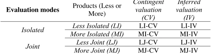
isolated mode s/he was then further allocated to the “More” or “Less” product. This 3x2
design is exhibited in Table 1. Each subject was only exposed to one of the treatments. In the
joint mode subjects evaluated the products “Less” and “More” simultaneously while in the
isolated mode subjects evaluated either the “Less” or the “More” product but not both (i.e.,
three treatments: 1. Less & More-joint, 2. More-isolated, 3. Less-isolated).
In each treatment, subjects were asked to evaluate two product categories (olive oil
and apples). Order was alternated between subjects. The specific products used are exhibited
in Table 2. Under the “More” modes, the superior quality products and the inferior
counterpart were tied together and presented as a single product, thus we refer to the “More”
product as a single product from now on. Standard socio-demographic data were also
collected. Appendix C exhibits photo stimuli of the products shown to subjects.
Our full factorial design is a 3x2x2 design4. In all, it took twelve subjects to complete
the full factorial design one time. An example is given in Appendix B (Table B1). As
exhibited, twelve subjects are required to participate in six treatments for two quality
products (BIO and PDO).
To sum up, in the “Isolated” evaluation modes subjects report their valuation either
for a quality food product (LI for Less-Isolated) or for a quality food product tied with a
smaller quantity of a conventional product (MI for More-Isolated) (see Table 2). In the
“Joint” evaluation modes subjects report their valuation for both the quality food product (LJ
4
9
for Less-Joint) as well as the quality product tied together with a conventional product (MJ
for More-Joint). This design was ran for two quality products (BIO and PDO) and two
elicitation methods (CV and IV).
We should note that while the additional conventional food product is of lower
quality than the PDO or BIO counterparts, in aggregate, the superior food quality product
tied with the lower quality product have a greater market value than the superior food quality
product itself. In the “Joint” evaluation mode, subjects evaluate the exact same products as in
treatments LIandMI but this time side by side.
No subject participated in more than one treatment. In addition, subjects evaluated the
products using either CV or IV method; that is, no subject reported valuations with both
methods. Third, each subject reported his/her valuation for one quality product, either a PDO
product or a BIO product but not both. However, each subject reported valuations for two
product categories i.e., olive oil and apples. Lastly, order of appearance of valuation
questions (and products) was alternated in order between subjects.
Field Experiment 1: The Survey
WTP was elicited in an actual market place just before subjects enter a super-market.
Interviews took place at various locations throughout the city, at stores of the three of the
biggest food retailers in the country. The interviews were conducted by a single proctor (one
of the authors) from Monday to Saturday, during morning and afternoon hours5. In total, 588
completed questionnaires were collected. Table 3 depicts socio-demographic information
from this sample.
5
10
WTP was elicited using a payment card format in which subjects selected their most
preferred choice among a series of sixteen price intervals (an example of the exact wording
of the valuation questions are exhibited in Appendix G). We chose the payment card format
instead of the single- or double-bounded approach because it exhibits more desirable
properties than the other two (Reaves et al. 1999), less yeah saying at high bid amounts
(Zhongmin et al. 2006) and more conservative estimates (Blaine et al. 2005). We designed
two payment cards, one for each product i.e., olive oil and apples (see Appendix D). The
payment card intervals were constructed using an exponential response scale to avoid range
and centering bias with classical uniform payment cards (Rowe et al. 1996). Drichoutis et al.
(2009) describe the procedure of constructing an exponential card in detail. The prices were
selected so as to cover a wide range of market prices for conventional and BIO/PDO olive oil
and apples, respectively.
To distinguish between experienced and inexperienced people we asked subjects to
self-rate their knowledge about either BIO or PDO products by asking them to indicate
whether they agree with the statement “I know a lot about these products” on a 1 to 5 scale
anchored by completely disagree and completely agree. Subjects that indicated to agree or
completely agree with the statement where categorized as familiar with the products and thus
experienced.
To isolate normative motivations for BIO and PDO products, we asked subjects to
indicate whether they agree with the statement “I should be looking to buy these products”
on a 1 to 5 scale anchored by completely disagree and completely agree. Subjects that
indicated to agree or completely agree with the statement where categorized as having strong
11
To proxy commitment costs we asked respondents to indicate how often they tend to
buy BIO or PDO olive oil and apple products on a likert scale ranging from 1 to 5 (never,
rarely, sometimes, often, always). Subjects that indicated buying often or always were
classified as having low commitment costs. An assumption in our approach is that peoples’
previous purchases of goods in a product category are an appropriate proxy of commitment
costs (similar to Lusk and Norwood 2009a). When people buy a product more often
commitment costs are low. With the IV method subjects are asked to predict WTP for the
“average consumer”. Therefore, if the person being asked thinks s/he is less price sensitive
than the “average” shopper, this may result in stating a lower WTP in the IV than in the CV.
For this reason price sensitivity was also recorded by having subjects answer a 5 point-likert
question regarding how often they take price under consideration while grocery shopping.
Answers were anchored by never and always and subjects that answered often or always
were classified as price sensitive.
Field Experiment 2: Design issues
In FE 2 we followed the same experimental design of FE 1 (see Table 1) with some
modifications for the valuation products. First, in order to make the “inferiority” of the low
quality product more salient, we tied the organic olive oil with a seed oil (instead of a
conventional oil). Seed oils are widely considered inferior quality products in the country as
compared to olive oil.
In addition, since the products used up to now are sold by their weight and volume,
we introduced eggs (instead of apples) as the second valuation product. Eggs are sold by
number of items. This allows us to more closely mimic List’s (2002) and Alevy et al.’s
12
Therefore, in each treatment subjects were asked to evaluate two product categories
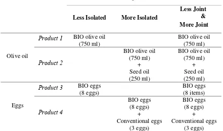
(olive oil and eggs) in alternating order. The specific products used are exhibited in Table 4.
The design in FE 2 closely mimics that of FE 1, with the exception that we only elicit
valuations for BIO products and not PDO. Appendix C exhibits photo stimuli of the products
shown to subjects.
Our full factorial design is a 3x2 design6. In all, it took six subjects to complete the
full factorial design one time. An example is given in Appendix B (Table B2). As exhibited,
six subjects are required to participate in six treatments for the organic quality product.
We should note that while the additional inferior food products are of lower quality
than the BIO counterparts, in aggregate, the superior food quality product tied with the lower
quality product have a greater market value than the superior food quality product itself. In
the “Joint” evaluation mode, subjects evaluate the exact same products as in treatments LI
andMI but this time side by side.
No subject participated in more than one treatment. In addition, subjects evaluated the
products using either CV or IV methods; that is, no subject reported valuations with both
methods. Third, each subject reported valuations for two product categories i.e., olive oil and
eggs. Lastly, order of appearance of valuation questions (and products) was completely
randomized.
Field Experiment 2: The Survey
6
13
WTP was elicited in an actual market place just before subjects enter a super-market.
Interviews were conducted by the same proctor as in FE 1. In total, 192 completed
questionnaires were collected. Table 3 depicts socio-demographic information from this
sample.
WTP was elicited using a similar payment card format to FE 1 (see Appendix D);
payment card intervals were constructed using an exponential response scale. For olive oil
the payment card was the same as in FE 1. The prices for eggs were selected so as to cover a
wide range of market prices for conventional and organic eggs.
Similar questions to FE 1 were asked to distinguish between experienced and
inexperienced subjects, to isolate normative motivations and proxy commitment costs.
III. Hypotheses and Results
Before proceeding with testing our hypotheses, insights can be gained by looking at some
descriptive statistics of the WTP responses. Figures 1a,b and 2a,b show the distribution of
responses over the 16-cell payment cards for olive oil in FE 1 and FE 2 respectively (similar
figures are available in Appendix F for apples and eggs). If one closely observes the figures,
it is apparent that for the “Joint” mode the distribution of responses for “More” is shifted
more to the right, as compared with the distribution of responses for the “Less” mode. This
indicates that WTP for the “More” product is greater than WTP for the “Less” product when
products are evaluate jointly. Surprisingly, there is a similar pattern for the “Isolated” mode
indicating the absence of a preference reversal. In addition, there is a clear shift of the
distribution of responses to the right for the inferred valuation method as compared to the
14
More or Less). This indicates that valuations elicited with the inferred method appear to be
greater than valuations elicited with the contingent method which refutes our basic
assumption that inferred valuation mitigates social desirability bias.
Before moving to the conditional analysis it is also important to investigate how the
goods and subjects in both field experiments vary along key variables i.e., experience of the
subject, normative motivations and commitment costs. Overall, results indicate that people
felt more experienced with BIO products (mean=3.43) than PDO products (mean=2.91).
p-values from a Wilcoxon-Mann-Whitney (WMN) test (p=0.0) indicate that there is a
significant difference between degree of familiarity for the two products. In addition, subjects
from FE 2 were slightly more experienced (mean=3.64) than subjects from FE 1
(mean=3.43) with respect to BIO products. A WMN test (p=0.03) indicates that the
difference is significant.
Results also indicate that people felt higher normative motivations for BIO products
(mean=2.81) than PDO products (mean=2.55). p-values from a WMN test (p=0.02) indicate
that the difference is statistically significant. However, motivations for BIO products were
not significantly different between field experiments (p=0.15 from WMN test).
With respect to commitment costs, subjects indicated lower commitment costs for PDO
olive oil (mean=2.11) than BIO olive oil (mean=1.69) and the difference is statistically
significant according to a WMN test (p=0.0)7. However, for apples it is the exact opposite
since subjects indicate lower commitment costs for BIO apples (mean=2.45) than PDO
apples (mean=1.91) and the difference is statistically significant according to a WMN test
(p=0.0). In addition, subjects in the first FE exhibited lower commitment costs for BIO olive
7
15
oil (mean=1.69) than the second FE (mean=1.33) and the difference is statistically significant
(p=0.01 from WMN test).
To formally test our hypothesis for preference reversals we adopt the definitions from
Alevy et al. (2011):
Definition 1: A strong evaluation mode effect is observed when, in aggregate,
preferences over the goods are: LI (Less, Isolated)MI (More, Isolated) and MJ (More,
Joint)LJ (Less, Joint).
Definition 2: A weak evaluation mode effect is observed when, in aggregate, preferences
over the bundles are: LI ~ MI and MJ LJ.
To test the effect of Inferred valuation on elicited valuations we can directly test whether
WTP WTP Inferred Contingent.
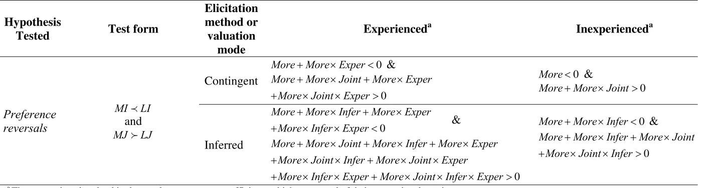
Table 5 summarizes the test forms that we adopt to test for preference reversals across
the contingent and inferred valuation methods (Appendix E shows detailed derivations).
Table E1 in the appendix shows the various linear combination forms that we use to test
whether InferredContingent (detailed derivations are exhibited in Appendix E as well). To
test these hypotheses we estimate an interval regression model (to take into account the
interval nature of the dependent variable) with robust clustered standard errors (to account
for multiple responses by the same person in the Joint treatments). The empirical
specification for FE 1 follows closely Alevy et al.’s (2011) specification:
1 2 3 4 5 6 7 8
9 10 11 12
13 14 15 16
i i i i i i i i
i i i i i i ii
i i i i i i
WTP a a More a Joint a Infer a Exper a BIO a Norm a Commit
a PrSens a BIO Exper a BIO Norm a BIO Commit
a BIO PrSens a Infer Norm a Infer Commit a Infer P
17 18 19 20
21 22 23
24 25
i
i i i i i i i i
i i i i i i i
i i i i i i
rSens
a Infer Exper a More Joint a More Infer a More Exper
a Joint Infer a Joint Exper a More Joint Infer
a More Joint Exper a More Infer Exper a
26
27 28
i i i
i i i i i i
Joint Infer Exper
a More Joint Infer Exper a OrderQuest u
b'DEM
16
The DEM vector is a vector of demographic variables described in Table 3. The More,
Joint, Infer, Exper, BIO, Norm, Commit and PrSens variables are dummies indicating
conditions consistent with the variable name i.e., evaluation of the “More” product (vs. the
“Less” product), evaluation in the “Joint” mode (vs. the “Isolated” mode), evaluation using
the Inferred elicitation method (vs. Contingent valuation), experienced consumers (vs.
inexperienced consumers), evaluation of organic products (vs. PDO), subject has high
normative motivations for the product (vs. low normative motivations), subject has low
commitment costs with the product (vs. high commitment costs) and subject is price sensitive
(vs. no price sensitivity) respectively. The OrderQuest variable is a dummy controlling for
the order of the valuation questions between product categories (olive oil and apples in FE
1/olive oil and eggs in FE 2).
A similar specification was adopted for FE 2 without the BIO and PrSens dummies and
its interactions (only organic products were evaluated in FE 2). In addition, we didn’t ask the
price sensitivity question in FE 2 because we didn’t find it playing a significant role in FE 1.
To test our hypothesis, we use specification (1) to derive linear combinations of
coefficients for hypothesis testing which are exhibited in detail in Appendix E. Since the
focus is on testing the significance of linear combinations of coefficients, results from the
raw interval regression output of equation (1) (and the respective equation for FE 2) are
shown in Appendix A.
Does CV and IV generate consistent preference orderings?
To answer this question we test the hypotheses as described in Table 5. Notice that this
test requires checking two hypotheses; a confirmation of inconsistent preference orderings
17
from Field Experiment 1. The interaction terms associated with the Experience dummy
allows us to further disentangle the effect of market experience on preference reversals. For
each product (olive oil and apples) and method (contingent and inferred valuation) we first
test whether the respective linear combination of coefficients from Table 5 is 0
(H0:Linear Comb.0). The alternative hypothesis (H1:Linear Comb.0) is consistent
with MILI. We then test whether the respective linear combination of coefficients is 0
(H0:Linear Comb.0). The alternative hypothesis (H1:Linear Comb.0) is consistent
with MJLJ . Note that any p-value exhibited in the table implies
1pvalue
for thealternative hypothesis.
First notice that the majority of linear combinations of coefficients are evaluated as
positive which implies that MILI and MJ LJ. More specifically, most hypothesis
involving H0: WTP in MI mode > WTP in LI mode, cannot be rejected which suggests that
average WTP in the MI mode is statistically significantly higher than average WTP in the LI
mode8. However, there are some exceptions: medium sized p-values (or p-values >10% & <
90%) indicate that we can neither reject H0 nor H1. In turn, this implies that MI~LI. On
the other hand, the hypothesis involving H0: WTP in MJ mode < WTP in the LJ mode, is
rejected in all but one cases, implying that MJ LJ. Overall our findings indicate that we
never observe strong evaluation mode effects as was the case in List (2002) (as well as Alevy
et al., (2011)). Note that direct comparisons should be done in caution since, in contrast to
those studies, we didn’t offer salient payments for eliciting valuations.
8
18
However, we do observe weak evaluation mode effects (that is, MI~LI & MJ LJ). It
is worth noting that weak preference reversals are observed only for the inferred valuation
method and for experienced subjects. There are two conclusions coming out of these results.
The first one is that market experience does not play a significant role in FE 1 for the
contingent valuation method. It appears that both experienced and inexperienced consumers
were not likely to commit a preference reversal in aggregate. The second conclusion is
related to the fact that we find weak preference reversals for experienced subjects in the
inferred elicitation method. This makes sense if we assume that experienced subjects are
more likely to expect others to fall prey to social desirability bias and thus predict for others
that, in aggregate, MI~LI. On the other hand, inexperienced subjects may not expect other
people to fall for social desirability bias and thus predict MILI.
Data from Field Experiment 2 can help test the robustness of our results from FE 1. In
FE 2 we made two significant changes: (a) the inferiority of the lower quality product was
made more salient for olive oil by using seed oil instead of conventional olive oil and (b)
eggs were used instead of apples to test whether the sell-by-items nature of the product
(similar to List’s (2002) and Alevy et al.’s (2011) itemized card bundles) would make a
difference.
Results are exhibited in Table 6b. The pattern is somewhat different from FE 1 in that
we observe more often weak preference reversals. First note that all p-values associated with
the hypothesis H0: WTP in MJ mode < WTP in the LJ mode, are lower than 5% indicating
that the null hypothesis is highly rejected and that MJ LJ. However, p-values for H0:
WTP in MI mode > WTP in LI mode, are, in most cases, much lower than FE 1 and further
away from conventional significance levels. In essence, this implies that average WTP in the
19
The conclusions we can draw from FE 2 are product specific. For valuations elicited
with the CV method, we observe weak preference reversals for olive oil and no preference
reversals for eggs and results are invariant for experienced/inexperienced subjects. These
results may mean that making the inferiority of one of the products more salient significantly
affected consumers, in aggregate, in generating inconsistent preference orderings (remember
that in FE 1 we found no preference reversals for olive oil in the CV method). However,
itemizing the product was not a contributing factor in generating inconsistent preference
orderings.
On the other hand, we observe weak preference reversals for valuations elicited with the
IV method in all but one cases. Predictions elicited by experienced subjects for olive oil
generated consistent preference orderings.
Overall, while we can’t replicate strong evaluation mode effects as in List (2002) and
Alevy et al. (2011) we do observe weak evaluation mode effects. It also appears that the IV
method is more susceptible in generating inconsistent preference orderings than the CV
method. Market experience didn’t make much difference in our results, as in the original
studies.
Does IV generate lower valuations than CV?
The aim of the inferred valuation method, as originally used, was to mitigate social
desirability bias that is encompassed in hypothetical bias. Lusk and Norwood (2009a,b)
found that for goods with high normative motivations IV generated lower WTP valuations
than hypothetical own valuations. Therefore, for goods for which people have high normative
motivations we would expect average WTP from IV to be lower than average WTP from
20
motivations for the good we would expect InferredContingent (see also Figure 1 in Lusk
and Norwood, 2009a). Table E1 in the appendix indicates linear combinations of coefficients
that are required to test our hypothesis, by evaluation mode, subjects experience, normative
motivations, commitment costs and price sensitivity. Results of these one-sided tests are
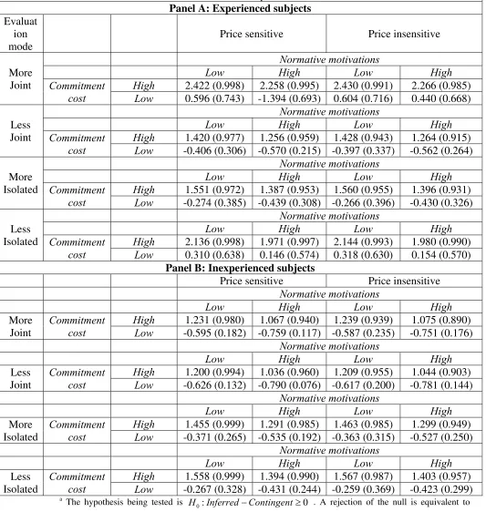
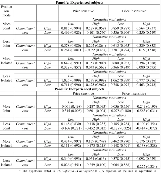
displayed in tables 7a,b for FE 1 and tables 7c,d for FE 2. A positive value indicates that
InferredContingent while a negative value indicates the exact opposite.
Visual inspection of Tables 7 indicates that the linear combination of coefficients often
results in a positive value indicating that WTP from the IV method is greater than WTP from
the CV method. However, Table 7 also exhibits negative values indicating that average WTP
from IV is lower than average WTP from CV. This is most often the case for inexperienced
subjects and/or with high normative motivations and/or low commitment costs. P-values can
help us decide whether the observed differences are statistically significant given the
dispersions. The hypothesis being tested is H0:InferredContingent0, therefore a high
p-value (90%) indicates that InferredContingent, a low p-value (10%) indicates
rejection of the null while an intermediate-sized p-vlaue (10% p value90%) indicates
that WTP Inferred=WTP Contingent.
Tables 7a,b (corresponding to FE 1) indicate that for high commitment costs, the IV
method generates WTP values that are statistically significantly greater than the CV method.
This finding applies equally to experienced and inexperienced subjects. However, for
inexperienced subjects in the majority of cases for which commitment costs are low, WTP
values elicited with the IV method are statistically significantly lower than the CV method.
Moreover, this finding is often the case when normative motivations are high rather than low.
21
are low, values elicited with IV are statistically indistinguishable than values elicited with
CV.
These findings are further reinforced in FE 2 but we also find some notable differences.
For olive oil, results show that for subjects with low commitment costs, in aggregate, IV
generates valuations lower than CV, especially when normative motivations are high as well.
On the other hand, in case of low normative motivations and high commitment costs we find
that WTP values from IV are higher than CV. This finding applies equally to experienced
and inexperienced subjects. For eggs we never find that IV generates values statistically
significantly lower than CV, which may be an indication that the nature of the product (e.g.,
sold by number of items vs. sold by volume) also has an effect on subjects’ valuations.
In sum, we partially reconfirm Lusk and Norwood’s (2009a,b) results that found that
for goods with high normative motivations we should expect IV to generate lower valuations
than CV. However, their model did not predict that for high commitment costs and low
normative motivations there could be a case that IV generates higher valuations that CV.
This calls for further scrutiny of the IV method with more diverse samples and goods.
IV. Conclusions
We started this article with a series of questions which we are now ready to answer. In
both field experiments we could not replicate strong evaluation mode effects as in the
original studies that studied preference reversals (List, 2002; Alevy et al. 2011). In our
experiments, we only observe weak evaluation mode effects. It also appears that the IV
method is slightly more susceptible in generating inconsistent preference orderings than the
22
Our second aim was to reexamine the effectiveness of the IV method in mitigating
social desirability bias. Inferred valuation consistently generated higher valuations than
Contingent valuation in the case where the commitment cost was high. On the other hand,
with low commitment cots and high normative motivations, inferred valuation successfully
mitigated social desirability by generating lower valuations than CV. To the extent that
hypothetical bias and social desirability bias was present in our study (and we have no reason
to believe that our study would differ from other hypothetical studies) this is a sign that IV
will work for certain products and consumers.
It will take time and more studies of this kind to answer the question for which
contexts, products and samples the inferred valuation method remains a promising method
for mitigating biases. All in all, we believe that this topic could indeed be a prime area for
23
References
Alevy, J.E.; J. List and W. Adamowicz. 2011. "How Can Behavioral Economics Inform
Non-Market Valuation;an Example from the Preference Reversal Literature." Land
Economics, 87(3), 365-381.
Blaine, T.W.; F.R. Lichtkoppler; K.R. Jones and R.H. Zondag. 2005. "An Assessment of Household Willingness to Pay for Curbside Recycling: A Comparison of Payment Card and
Referendum Approaches." Journal of Environmental Management, 76(1), 15-22.
Caswell, Julie A. and E. M. Modjuzska. 1996. "Using Informational Labeling to Influence
the Market for Quality in Food Products." American Journal of Agricultural Economics, 78
1248-1253.
Crowne, D. P. and D Marlowe. 1960. "A New Scale of Social Desirability Independent of
Psychopathalogy." Journal of Consulting Psychology, 24(4), 349-50.
Darby, M. and E. Karni. 1973. "Free Competition and Optimal Amount of Fraud." Journal
of Law and Economics, 16, 67-88.
Drichoutis, Andreas C.; Panagiotis Lazaridis and Rodolfo M. Nayga, Jr. 2009. "On
Consumers' Valuation of Nutrition Information." Bulletin of Economic Research, 61(3),
223-247.
Fisher, R. J. . 1993. "Social Desirability Bias and the Validity of Indirect Questioning."
Journal of Consumer Research, 20(2), 303-15.
Grether, D. M. and C. R. Plott. 1979. "Economic Theory of Choice and the Preference
Reversal Phenomenon." American Economic Review, 69(4), 623-38.
Hsee, C. K.; G. F. Loewenstein; Sally Blount and Max H. Bazerman. 1999. "Preference Reversals between Joint and Separate Evaluations of Options: A Review and Theoretical
Analysis." Psychological Bulletin, 125, 576-591.
Hsee, C.K. 1996. "The Evaluability Hypothesis: An Explanation for Preference Reversals
between Joint and Separate Evaluations of Alternatives." Organizational Behavior and
24
Johnson, Eric J.; Mary Steffel and Daniel G. Goldstein. 2005. "Making Better Decisions:
From Measuring to Constructing Preferences." Health Psychology, 24(4), S17–S22.
Leggett, C. G.; N. S. Kleckner; K. J. Boyle; J. W. Duffield and R. C. Mitchell. 2003. "Social Desirability Bias in Contingent Valuation Surveys Administered through in-Person
Interviews." Land Economics,79(4), 561-75.
Lichtenstein, S. and P. Slovic. 2006. The Construction of Preference. Cambridge, UK:
Cambridge University Press.
List, J.; R. Berrens; A. Bohara and J. Kerkvliet. 2004. "Examining the Role of Social
Isolation on Stated Preferences." American Economic Review, 94(3), 741-752.
List, J.A. 2002. "Preference Reversals of a Different Kind: The “More Is Less”
Phenomenon." American Economic Review, 92(5), 1636-1643.
List, J.A. 2002. "Preference Reversals of a Different Kind:The “More Is Less” Phenomenon."
The American Economic Review, 92(5), 1636-1643.
Lusk, J. and F. B. Norwood. 2009b. "An Inferred Valuation Method." Land Economics,
85(3), 500-514.
Lusk, JaysonL. and F. Bailey Norwood. 2009a. "Bridging the Gap between Laboratory
Experiments and Naturally Occurring Markets:An Inferred Valuation Method." Journal of
Environmental Economic and Management, 58, 236-50.
Payne, John W.; James R. Bettman and David A. Schkade. 1999. "Measuring Constructed
Preferences: Towards a Building Code." Journal of Risk and Uncertainty, 19(1), 243-270.
Plant, E. A.; P. G. Devine and P. C Brazy. 2003. "The Bogus Pipeline and Motivations to
Respond without Prejudice: Revisiting the Fading and Faking of Racial Prejudice." Group
25
Reaves, D.W.; R.A. Kramer and T.P. Holmes. 1999. "Does Question Format Matter?
Valuing an Endangered Species." Environmental and Resource Economics 14(3), 365-83.
Rowe, R.D.; W.D. Schulze and Breffle. 1996. "A Test for Payment Card Biases." Journal of
Environmental Economics and Management, 31, 178-85.
Seidl, Christian. 2002. "Preference Reversal." Journal of Economic Surveys, 16(5), 621-655.
Slovic, P. and S. Lichtenstein. 1968. "Preference-Reversals: A Broader Perspective."
American Economic Review, 73(4), 596-605.
Slovic, Paul. 1995. "The Construction of Preference." American Psychologist, 50(5),
364-371.
Slovic, Paul and Sarah Lichtenstein. 1983. "Preference-Reversals: A Broader Perspective."
American Economic Review, 73(4), 596-605.
Zhongmin, X.; J. Loomis; Z. Zhiqiang and K. Hamamura. 2006. "Evaluating the Performance of Different Willingness to Pay Question Formats for Valuing Environmental
26
Table 1. Field experiments - experimental design
Elicitation method
Evaluation modes Products (Less or
More) Contingent valuation (CV) Inferred valuation (IV)
Isolated Less Isolated (LI) LI-CV LI-IV More Isolated (MI) MI-CV MI-IV
[image:27.612.72.532.153.666.2]Joint Less Joint (LJ) LJ-CV LJ-IV More Joint (MJ) MJ-CV MJ-IV
Table 2. Products by evaluation mode (FE 1)
Evaluation modes
Less Isolated More Isolated
Less Joint & More Joint
Olive oil
Product 1 BIO olive oil
(750 ml)
BIO olive oil (750 ml)
Product 2
BIO olive oil (750 ml)
+
Conventional olive oil (250 ml)
BIO olive oil (750 ml)
+
Conventional olive oil (250 ml)
Product 3 PDO olive oil
(750 ml)
PDO olive oil (750 ml)
Product 4
PDO olive oil (750 ml)
+
Conventional olive oil (250 ml)
PDO olive oil (750 ml)
+
Conventional olive oil (250 ml)
Apples
Product 5 BIO apples
(1 Kgr) BIO apples (1 Kgr) Product 6 BIO apples (1 Kgr) + Conventional apples (250 gr) BIO apples (1 Kgr) + Conventional apples (250 gr)
Product 7 PDO apples
(1 Kgr)
PDO apples (1 Kgr)
Product 8
PDO apples (1 Kgr )
27
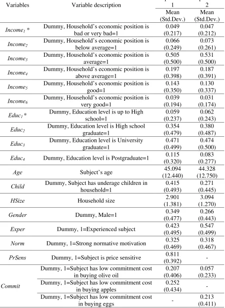
Table 3. Variable description
Variables Variable description
Field experiment 1 Field experiment 2 Mean (Std.Dev.) Mean (Std.Dev.)
Ιncome1*
Dummy, Household’s economic position is bad or very bad=1
0.049 (0.217)
0.047 (0.212)
Ιncome2
Dummy, Household’s economic position is below average=1
0.066 (0.249)
0.073 (0.261)
Ιncome3 Dummy, Household’s economic position is
average=1
0.505 (0.500)
0.531 (0.500)
Ιncome4
Dummy, Household’s economic position is above average=1
0.197 (0.398)
0.187 (0.391)
Ιncome5
Dummy, Household’s economic position is good=1
0.143 (0.350)
0.130 (0.337)
Ιncome6
Dummy, Household’s economic position is very good=1
0.039 (0.194)
0.031 (0.174)
Educ1 *
Dummy, Education level is up to High school=1 0.059 (0.237) 0.062 (0.243) Educ2
Dummy, Education level is High school graduate=1 0.354 (0.479) 0.380 (0.487) Educ3
Dummy, Education level is University graduate=1
0.471 (0.499)
0.474 (0.500)
Educ4 Dummy, Education level is Postgraduate=1 0.115
(0.320)
0.083 (0.277)
Age Subject’s age 45.094
(12.440)
44.328 (12.750)
Child Dummy, Subject has underage children in
household=1
0.415 (0.493)
0.271 (0.445)
HSize Household size 2.901
(1.381)
3.094 (1.270)
Gender Dummy, Male=1 0.349
(0.477)
0.266 (0.443)
Exper Dummy, 1=Experienced subject 0.423 (0.495)
0.547 (0.499)
Norm Dummy, 1=Strong normative motivation 0.325 (0.469)
0.318 (0.467)
PrSens Dummy, 1=Subject is price sensitive 0.811
(0.392) -
Commit
Dummy, 1=Subject has low commitment cost in buying olive oil
0.207 (0.406)
0.057 (0.233) Dummy, 1=Subject has low commitment cost
in buying apples
0.252
(0.434) -
Dummy, 1=Subject has low commitment cost
in buying eggs -
0.213 (0.411)
28
Table 4. Products by evaluation mode (FE 2)
Treatments per evaluation modes
Less Isolated More Isolated
Less Joint & More Joint
Olive oil
Product 1 BIO olive oil
(750 ml)
BIO olive oil (750 ml)
Product 2
BIO olive oil (750 ml)
+ Seed oil (250 ml)
BIO olive oil (750 ml)
+ Seed oil (250 ml)
Eggs
Product 3 BIO eggs
(8 eggs)
BIO eggs (8 items)
Product 4
BIO eggs (8 eggs)
+
Conventional eggs (3 eggs)
BIO eggs (8 eggs)
+
29
Table 5. Linear combinations of coefficients for hypothesis testing
Hypothesis
Tested Test form
Elicitation method or valuation
mode
Experienceda Inexperienceda
Preference reversals
MILI
and
MJ LJ
Contingent
0
MoreMore Exper &
0
More More Joint More Exper More Joint Exper
0
More &
0
MoreMore Joint
Inferred
0
More More Infer More Exper More Infer Exper
&
0
More More Joint More Infer More Exper More Joint Infer More Joint Exper
More Infer Exper More Joint Infer Exper
0
MoreMore Infer &
0
More More Infer More Joint More Joint Infer
a
30
Table 6a. Hypothesis tests for preference reversals in Field Experiment 1
Olive oil Apples
Experienced Inexperienced Experienced Inexperienced
(p-value)
CV
Ho : WTP in MI mode >
WTP in the LI mode
(isolated) 1.372 (0.998) 1.504 (0.999) 0.341 (0.990) 0.545 (0.999)
Ho : WTP in MJ mode <
WTP in the LJ mode
(joint) 0.571 (0.051) 1.081 (0.000) 0.080 (0.262) 0.467 (0.000) IV
Ho : WTP in MI mode >
WTP in the LI mode
(isolated) 0.787 (0.868) 1.400 (0.999) -0.041 (0.432) 0.630 (0.999)
Ho : WTP in MJ mode <
WTP in the LJ mode
(joint) 1.572 (0.000) 1.112 (0.000) 0.314 (0.001) 0.319 (0.000)
Table 6b. Hypothesis tests for preference reversals in Field Experiment 2
Olive oil Eggs
Experienced Inexperienced Experienced Inexperienced
(p-value)
CV
Ho : WTP in MI mode >
WTP in the LI mode
(isolated) 0.075 (0.521) 0.704 (0.718) 1.045 (0.958) 1.081 (0.934)
Ho : WTP in MJ mode <
WTP in the LJ mode
(joint) 0.526 (0.016) 0.614 (0.005) 0.318 (0.020) 0.341 (0.000) IV
Ho : WTP in MI mode >
WTP in the LI mode
(isolated) 2.073 (0.983) -0.160 (0.449) 0.241 (0.644) -0.281 (0.343)
Ho : WTP in MJ mode <
WTP in the LJ mode
[image:31.612.41.538.367.628.2]31
Table 7a. Hypothesis test for whether IV generates lower valuations than CVa,b
Olive oil – Field Experiment 1
Panel A: Experienced subjects
Evaluat ion mode
Price sensitive Price insensitive
More Joint
Normative motivations
Low High Low High Commitment
cost
High 2.422 (0.998) 2.258 (0.995) 2.430 (0.991) 2.266 (0.985)
Low 0.596 (0.743) -1.394 (0.693) 0.604 (0.716) 0.440 (0.668)
Less Joint
Normative motivations
Low High Low High Commitment
cost
High 1.420 (0.977) 1.256 (0.959) 1.428 (0.943) 1.264 (0.915)
Low -0.406 (0.306) -0.570 (0.215) -0.397 (0.337) -0.562 (0.264)
More Isolated
Normative motivations
Low High Low High Commitment
cost
High 1.551 (0.972) 1.387 (0.953) 1.560 (0.955) 1.396 (0.931)
Low -0.274 (0.385) -0.439 (0.308) -0.266 (0.396) -0.430 (0.326)
Less Isolated
Normative motivations
Low High Low High Commitment
cost
High 2.136 (0.998) 1.971 (0.997) 2.144 (0.993) 1.980 (0.990)
Low 0.310 (0.638) 0.146 (0.574) 0.318 (0.630) 0.154 (0.570)
Panel B: Inexperienced subjects
Price sensitive Price insensitive
Normative motivations
Low High Low High
More Joint
Commitment cost
High 1.231 (0.980) 1.067 (0.940) 1.239 (0.939) 1.075 (0.890)
Low -0.595 (0.182) -0.759 (0.117) -0.587 (0.235) -0.751 (0.176)
Normative motivations
Low High Low High
Less Joint
Commitment cost
High 1.200 (0.994) 1.036 (0.960) 1.209 (0.955) 1.044 (0.903)
Low -0.626 (0.132) -0.790 (0.076) -0.617 (0.200) -0.781 (0.144)
Normative motivations
Low High Low High
More Isolated
Commitment cost
High 1.455 (0.999) 1.291 (0.985) 1.463 (0.985) 1.299 (0.949)
Low -0.371 (0.265) -0.535 (0.192) -0.363 (0.315) -0.527 (0.250)
Normative motivations
Low High Low High
Less Isolated
Commitment cost
High 1.558 (0.999) 1.394 (0.990) 1.567 (0.987) 1.403 (0.957)
Low -0.267 (0.328) -0.431 (0.244) -0.259 (0.369) -0.423 (0.299)
a
The hypothesis being tested is H0:InferredContingent0 . A rejection of the null is equivalent to
1:
H InferredContingent. Table E1 in the appendix shows the exact linear combination of coefficients being tested in each case.
b
32
Table 7b. Hypothesis testing whether IV generates lower valuations than CVa,b
Apples – Field Experiment 1
Panel A: Experienced subjects
Evaluat ion mode
Price sensitive Price insensitive
More Joint
Normative motivations
Low High Low High Commitment
cost
High 0.813 (0.994) 0.527 (0.959) 0.850 (0.987) 0.564 (0.937)
Low 0.499 (0.923) -0.101 (0.760) 0.536 (0.906) 0.250 (0.749)
Less Joint
Normative motivations
Low High Low High Commitment
cost
High 0.578 (0.980) 0.292 (0.864) 0.615 (0.965) 0.329 (0.838)
Low 0.264 (0.801) -0.022 (0.467) 0.301 (0.794) 0.015 (0.518)
More Isolated
Normative motivations
Low High Low High Commitment
cost
High 0.642 (0.991) 0.357 (0.909) 0.680 (0.983) 0.394 (0.888)
Low 0.328 (0.857) 0.043 (0.562) 0.366 (0.849) 0.080 (0.595)
Less Isolated
Normative motivations
Low High Low High Commitment
cost
High 1.025 (0.999) 0.739 (0.999) 1.062 (0.999) 0.777 (0.996)
Low 0.711 (0.996) 0.425 (0.962) 0.748 (0.992) 0.463 (0.942)
Panel B: Inexperienced subjects
Price sensitive Price insensitive
Normative motivations
Low High Low High
More Joint
Commitment cost
High -0.001 (0.498) -0.287 (0.093) 0.036 (0.556) -0.249 (0.195)
Low -0.315 (0.096) -0.601 (0.004) -0.278 (0.180) -0.563 (0.031)
Normative motivations
Low High Low High
Less Joint
Commitment cost
High 0.148 (0.830) -0.138 (0.233) 0.185 (0.784) -0.100 (0.354)
Low -0.166 (0.221) -0.452 (0.013) -0.129 (0.325) -0.414 (0.072)
Normative motivations
Low High Low High
More Isolated
Commitment cost
High 0.424 (0.997) 0.139 (0.749) 0.462 (0.970) 0.176 (0.727)
Low 0.111 (0.692) -0.175 (0.218) 0.148 (0.691) -0.138 (0.328)
Normative motivations
Low High Low High
Less Isolated
Commitment cost
High 0.340 (0.993) 0.054 (0.613) 0.378 (0.945) 0.092 (0.629)
Low 0.026 (0.551) -0.259 (0.100) 0.064 (0.588)
-0.222 (0.224)
a
The hypothesis tested is H0:InferredContingent0 . A rejection of the null is equivalent to
1:
H InferredContingent. Table E1 in the appendix shows the exact linear combination of coefficients being tested in each case.
b
33
Table 7c. Hypothesis testing whether IV generates lower valuations than CVa,b
Olive oil – Field Experiment 2
Panel A: Experienced subjects
Evaluation mode More Joint Normative motivations Low High Commitment cost
High 5.071 (0.999) 2.949 (0.974)
Low 1.431 (0.685) -0.690 (0.396)
Less Joint
Low High Commitment
cost
High 4.667 (0.999) 2.545 (0.964)
Low 1.028 (0.639) -1.094 (0.333)
More Isolated
Low High
Commitment cost
High 3.881 (0.996) 1.760 (0.864)
Low 0.242 (0.540) -1.880 (0.179)
Less Isolated
Low High
Commitment cost
High 1.883 (0.945) -0.239 (0.427)
Low -1.756 (0.264) -3.878 (0.058)
Panel B: Inexperienced subjects
More Joint
Normative motivations
Low High
Commitment cost
High 4.597 (0.999) 2.475 (0.949)
Low 0.957 (0.624) -1.164 (0.334)
Less Joint
Low High
Commitment cost
High 3.911 (0.998) 1.789 (0.892)
Low 0.271 (0.537) -1.850 (0.239)
More Isolated
Low High
Commitment cost
High 1.619 (0.886) -0.502 (0.383)
Low -2.020 (0.242) -4.142 (0.064)
Less Isolated
Low High
Commitment cost
High 2.483 (0.988) 0.362 (0.598)
Low -1.156 (0.335) -3.278 (0.097)
a
The hypothesis tested is H0:InferredContingent0 . A rejection of the null is equivalent to
1:
H InferredContingent. Table E1 in the appendix shows the exact linear combination of coefficients being tested in each case.
b
34
Table 7d. Hypothesis testing whether IV generates lower valuations than CVa,b Eggs – Field Experiment 2
Panel A: Experienced subjects
Evaluation mode More Joint Normative motivations Low High Commitment cost
High 0.778 (0.864) 0.192 (0.596)
Low 0.792 (0.795) 0.206 (0.625)
Less Joint
Low High Commitment
cost
High 0.480 (0.762) -0.106 (0.446)
Low 0.494 (0.704) -0.092 (0.440)
More Isolated
Low High
Commitment cost
High 0.828 (0.873) 0.242 (0.601)
Low 0.842 (0.789) 0.256 (0.610)
Less Isolated
Low High
Commitment cost
High 1.632 (0.991) 1.046 (0.859)
Low 1.646 (0.950) 1.060 (0.876)
Panel B: Inexperienced subjects
More Joint
Normative motivations
Low High
Commitment cost
High 1.727 (0.961) 1.141 (0.825)
Low 1.740 (0.954) 1.154 (0.881)
Less Joint
Low High
Commitment cost
High 1.162 (0.899) 0.576 (0.692)
Low 1.176 (0.885) 0.590 (0.743)
More Isolated
Low High
Commitment cost
High 0.250 (0.665) -0.336 (0.372)
Low 0.264 (0.612) -0.322 (0.369)
Less Isolated
Low High
Commitment cost
High 1.612 (0.983) 1.026 (0.831)
Low 1.626 (0.936) 1.040 (0.843)
a
The hypothesis tested is H0:InferredContingent0 . A rejection of the null is equivalent to
1:
H InferredContingent. Table E1 in the appendix shows the exact linear combination of coefficients being tested in each case.
b
35 0 .0 5 .1 .1 5 .2 F rac ti on
1 2 3 4 5 6 7 8 9 10 11 12 13 14 15 16 Joint-More 0 .0 5 .1 .1 5 .2 F rac ti on
1 2 3 4 5 6 7 8 9 10 11 12 13 14 15 16 Joint-Less 0 .0 5 .1 .1 5 .2 F rac ti on
1 2 3 4 5 6 7 8 9 10 11 12 13 14 15 16 Isolated-More 0 .0 5 .1 .1 5 .2 F rac ti on
1 2 3 4 5 6 7 8 9 10 11 12 13 14 15 16 Isolated-Less
Olive oil - Field Experiment 1
Contingent Valuation
Figure 1a. Distribution of responses by payment card cells for olive oil in FE 1(Contingent valuation)
0 .0 5 .1 .1 5 .2 F rac ti on
1 2 3 4 5 6 7 8 9 10 11 12 13 14 15 16 Joint-More 0 .0 5 .1 .1 5 .2 F rac ti on
1 2 3 4 5 6 7 8 9 10 11 12 13 14 15 16 Joint-Less 0 .0 5 .1 .1 5 .2 F rac ti on
1 2 3 4 5 6 7 8 9 10 11 12 13 14 15 16 Isolated-More 0 .0 5 .1 .1 5 .2 F rac ti on
1 2 3 4 5 6 7 8 9 10 11 12 13 14 15 16 Isolated-Less
Olive oil - Field Experiment 1
[image:36.612.81.474.51.326.2]Inferred Valuation
[image:36.612.80.475.362.645.2]36 0 .1 .2 .3 .4 F rac ti on
1 2 3 4 5 6 7 8 9 10 11 12 13 14 15 16 Joint-More 0 .1 .2 .3 .4 F rac ti on
1 2 3 4 5 6 7 8 9 10 11 12 13 14 15 16 Joint-Less 0 .1 .2 .3 .4 F rac ti on
1 2 3 4 5 6 7 8 9 10 11 12 13 14 15 16 Isolated-More 0 .1 .2 .3 .4 F rac ti on
1 2 3 4 5 6 7 8 9 10 11 12 13 14 15 16 Isolated-Less
Olive oil - Field Experiment 2
Contingent Valuation
Figure 2a. Distribution of responses by payment card cells for olive oil in FE 2 (Contingent valuation)
0 .1 .2 .3 F rac ti on
1 2 3 4 5 6 7 8 9 10 11 12 13 14 15 16 Joint-More 0 .1 .2 .3 F rac ti on
1 2 3 4 5 6 7 8 9 10 11 12 13 14 15 16 Joint-Less 0 .1 .2 .3 F rac ti on
1 2 3 4 5 6 7 8 9 10 11 12 13 14 15 16 Isolated-More 0 .1 .2 .3 F rac ti on
1 2 3 4 5 6 7 8 9 10 11 12 13 14 15 16 Isolated-Less
Olive oil - Field Experiment 2