Analysis of Stochastic Model on a Two Unit Hot Standby Combined Hardware Software System

Analysis of Stochastic Model on a Two-Unit Hot

Standby Combined Hardware-Software System

Rajeev Kumar

Sudesh Kumari

Department of Mathematics, Department of Mathematics,

M.D. University, Rohtak-124001, INDIA M.D. University, Rohtak-124001, INDIA

ABSTRACT

This paper deals with a stochastic model for a two-unit hot standby combined hardware-software system in which one unit is operative and the other is hot standby. The operative unit may have hardware or software failures and goes to repair. This leads to degradation of the system and then hot standby unit is under operation. Further on hardware or software failures of the hot standby unit the system goes to complete failures. Various measures of performance of the system are obtained using semi-Markov process and regenerative point techniques. Numerical results and graphs pertaining to a particular case are also included.

General Terms

Stochastic Process

Keywords

Two-Unit Hot Standby System, Combined hardware-software system, reliability, mean up time, profit, semi-Markov and Regenerative point techniques.

1.

INTRODUCTION

In the recent years, a large number of hardware-software systems have been developed and adopted due to their practical applications and common man’s affordability and inherent reliability. A hardware-software system consists of hardware and software subsystems. Most of the modern systems like mobiles, computers, robots, missiles, rockets, electronic meters, washing machines etc. are improvement over hardware-software systems. Today society and its Institutions are becoming more and more depend on many such systems. A few of the numerous applications of the hardware and software systems are control of communications and transport systems, automated plants operations and even in routine activities e.g. reservation of tickets, computation of various bills and in business. All these things demands high reliability since failure of any can be costly and hazardous. At present it is a matter of great importance to produce and provide the cost-effective, efficient, user friendly hardware-software system having higher reliability.

For effective performance of the hardware-software system, both its hardware and software components must function with considerable reliability. As the hardware-software systems are more complex and the demand on their reliability has increased exponentially. For the reliability analysis of the one-unit hardware-software system, combined reliability model i.e. considering both hardware and software components were discussed by some researchers such as Boyd and Monahan [1], Friedman and Tran [2], Hecht and Hecht [3], Huang et al.[4], Iyer and Velardi [5], Kanoun and Ortalo-Borrel [6], Kumar and Malik [7], Kumar and Kumar [8], Martin and

Mathur [9], Teng et al. [10], Trivedi [11], Trivedi et al. [12], Welke et al. [13] etc. However, analysis of a two-unit hot standby hardware-software system with respect to its reliability, availability and profit has not been reported in the literature of reliability modeling.

Keeping this in view, in the present paper, a stochastic model for two identical units hot standby combined hardware-software system is analyzed. Initially, one unit is operative and other is hot standby and any one of the units may have a hardware or software component failure. On failure of a unit either due to hardware or software component failure, the system goes to degraded state and when both the units fails the system goes to complete failure. It is assumed here that hardware and software failures are independent of each other and occurs only due to hardware and software components, respectively. Further, it is assumed that there is single repair facility/engineer that handles all types of hardware or software failures and reaches the system in negligible time.

Other assumptions of the model are:

1. After each hardware/software repair, the system is as good as new.

2. If a unit is under repair, it does not work for the system.

3. The times to failures are exponentially distributed whereas recovery/repair time distributions are general.

4. All random variables are mutually independent. 5. Switching is perfect and instantaneous.

Various measures of system performance are obtained using semi Markov Process and regenerative point techniques. The expressions for various measures of system performance are obtained such as mean time to system failure, mean up time, expected number of software repairs, expected number of hardware repairs, expected number of visits by repairman. Expected profit incurred for the system is also computed using above measures. Various conclusions regarding reliability and profit of the system are drawn on the basis of graphical studies.

2.

NOTATIONS

O : Operative unit.

Fsr : Software failure is not recovered and unit

is under manual repair.

Fhr : Hardware failure is not recovered and

unit is under manual repair.

FsR : Software repair is continuing from the

FhR : Hardware repair is continuing from the

previous state.

FsW : Unit is under software failure and it is

waiting for repair.

FhW : Unit is under hardware failure and it is

waiting for repair. λs : Software failure rate.

λh : Hardware failure rate.

αs : Software repair rate.

αh : Hardware repair rate.

gs(t) : P.d.f. of time to software repair.

gh(t) : P.d.f. of time to hardware repair.

The transition diagram depicting the various states of the system is shown in the fig.1.The epochs of entry into the states 0, 1, 2 are regenerative points and thus the states 0, 1, 2 are regenerative states and 3, 4, 5, 6 are failed states.

3.

MEASURES OF THE SYSTEM

PERFORMANCE

3.1 Transition Probabilities

The transition probabilities pij are given by

By these transition probabilities it can be verified that

where

S = , S1 = , S2 = ,

3.2 Mean Sojourn Time

The mean sojourn time in the ith state is the expected first passage time taken by the unit at the ith state before transiting to any other state.

where Ti is the p.d.f. of device life time.

Therefore,

; ;

; ;

The unconditional mean time ( taken by the system to transition for any regenerative state j, when it (time) is counted from epoch of entrance into that state i is, mathematically, stated as:

Thus,

λ ; λ ; ; λ

4.

OTHER

MEASURES

OF

THE

SYSTEM PERFORMANCE

By probabilistic arguments for the regenerative process, the recursive relations for various measures of the system performance are obtained. Then on solving the relations using Laplace-Stieltjes transforms, we get the following measures:

Mean Time to System Failure

Mean Up Time

Expected Number of Hardware Repair

Expected Number of Software Repairs

Expected Number of Visits by the Repairman

where

5.

PROFIT ANALYSIS

The expected total profit (P0) incurred to the system in

steady state is given by

P0 =

where

C0 = revenue per unit up time of the system.

C1 = revenue per unit degradation time of the system.

C2 = cost per unit of hardware repair.

6.

PARTICULAR CASE

For the analysis purpose, the following particular case is taken:

_; The values of the various failure rates and repair rates are assumed as, i.e h=.01, h=.001, h=.002, s=.0002,

s=.002, αh=.2, αh=.6, αh=.8, αh= 1.8, αs=.3, αs=.5, αs=.6, αs=.7, C0 = 30000, C1= 30000, C2 = 500, C3= 300,

C4 = 20, C5 = 24000 etc.

7.

GRAPHICAL ANALYSIS

Using the above particular case and the assumed values of parameters, various graphs are plotted for mean time to system failure (T0), mean up time (A0), mean degradation

time (D0) and profit (P0) of the system for different values

of hardware and software failures rates (λh, λs) and repair

rates (αh , αs), respectively.

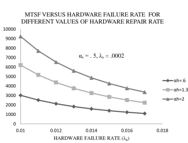
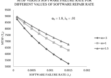
Fig. 2 and fig. 3 depicts the behavior of mean time to system failure (T0) with respect to various hardware and

software failure rates ( h , s ), respectively for different

values of hardware and software repair rates (αh , αs ). It

can be seen that mean time to system failure decreases as hardware and software failure rates increase and further mean time to system failure increases with higher values of repair rates.

Fig. 4 and fig. 5, shows the behavior of mean up time (A0)

with respect to various hardware and software failure rates ( h , s ), respectively for different values of hardware and

software repair rates (αh , αs ). From the graphs, it can be

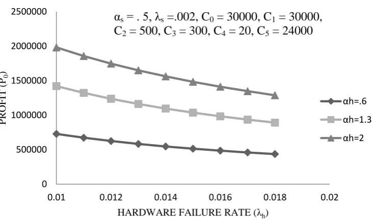
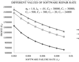
seen that mean up time decreases with the increase in the values of hardware and software failure rates and further mean up time increases with higher values of repair rates. Fig. 6 and fig. 7 reveals the pattern of the profit (P0)

incurred to the system with respect to hardware and software failure rates (h , s). It can be seen that the profit

(P0) of the system decreases as the failure rates increases

whereas increases for higher values of repair rates.

8.

CONCLUSIONS

It can be observed that reliability, mean up time and profit of the two unit hot standby hardware-software system decrease as hardware and software failure rates increases and these increases with higher values of hardware and software repair rates. The limits of hardware and software failure/repair rates can be obtained for the system to give positive profit that may be quite useful for both the system developer and the system user.

9.

REFERENCES

[1] Boyd, M.A. and Monahan, C. M., 1995 Developing Integrated Hardware-Software System Reliability models:

Difficulties and Issues [For Digital Avionics]. Proceeding of the Digital Avionics Systems Conference, 14th DASC, pp.193-198, Cambridge, USA.

[2] Friedman, M.A. and Tran, P., 1992. Reliability Techniques for Combined Hardware/Software Systems, Proceeding Annual Reliability and Maintainability Symposium, pp.290-293

[3] Hecht and Hecht, 1986. Software Reliability in The System Context, IEEE Transactions on Software Engineering, Vol.-12, pp.51-58.

[4] Huang, B., Li, X., Li, M., Bernstein, J. and Smidts, C.,2005. Study of the Impact of Hardware Fault on Software Reliability, Proc. 16th IEEE Int’l Symp. Software Reliability Engineering.

[5] Iyer, R.K. and Velardi, P., 1985. Hardware related Software Errors: Measurement and Analysis. IEEE Transactions on Software Engineering, Vol.11, pp.223-230.

[6] Kanoun, K. and Ortalo-Borrel, M., 2000. Fault-Tolerant System Dependency-Explicit Modeling of Hardware and Software Component-Interactions, IEEE Transactions Reliability, Vol. 49, No. 4, pp. 363-376.

[7] Kumar, A. and Malik, S.C., 2012. Stochastic Modeling of a Computer System with Priority to PM over S/W Replacement Subject to Maximum Operation and Repair, International Journal of Computer Applications, Vol.43, No.3, pp. 27-34.

[8] Kumar, R. and Kumar, M. 2012. Performance and Cost Benefit Analysis of a Hardware-Software System Considering Hardware based Software Interactions Failures and Different Types of Recovery, International Journal of Computer Applications, Vol. 53, No.-17, pp.25-32

[9] Martin, R. and Mathur, A.P., 1990. Software and Hardware Quality Assurance: Towards a Common Platform for Increase the Usability of this Methodology, Proc. IEEE Conf. Comm.

[10]Teng, X., Pham, H. and Jeske, D.R., 2006. Reliability Modeling of Hardware and Software Interactions and its Applications, IEEE Transactions Reliability, Vol.55, pp.571-577.

[11]Trivedi, K. S., Vasireddy, R., Trindade, D., Nathan,S., and Rick Castro., 2006. Modeling High Availability Systems. Proceeding Pacific Rim Dependability Conference PRDC. [12]Trivedi, K.S., 2011. Probability and Statistics with

Reliability, Queuing and Computer Science Applications, KPH Publishing.

[image:4.595.130.476.82.401.2]

: Operative State : Failed State : Degraded State : Regenerative Point

Fig. 1: State Transition Diagram

0 1000 2000 3000 4000 5000 6000 7000 8000 9000 10000

0.01 0.012 0.014 0.016 0.018

MT

SF

(T

0

)

HARDWARE FAILURE RATE (λ_h)

MTSF VERSUS HARDWARE FAILURE RATE FOR

DIFFERENT VALUES OF HARDWARE REPAIR RATE

αh=.6

αh=1.3

αh=2

α

s

= . 5, λ

s

= .0002

λ

h

F

sR

,F

hW

4

F

sR

,F

sW

3

F

hR

,F

sW

5

F

hr

,O

2

F

sR

,O

1

F

hR

,F

hW

6

g

h

(t)

2λ

h

2λ

s

g

s

(t)

g

s

(t)

g

h

(t)

λ

h

g

h

(t)

λ

s

g

s

(t)

λ

s

λ

s

[image:4.595.128.497.431.711.2]

[image:5.595.88.472.118.386.2] [image:5.595.90.443.464.710.2]

Fig. 3: MTSF Versus Software Failure Rate

Fig. 4: Mean Up Time Versus Hardware Failure Rate

5000 5500 6000 6500 7000 7500 8000 8500 9000 9500

0 0.0005 0.001 0.0015 0.002

MT

SF

(

T0

)

SOFTWARE FAILURE RATE (λ_s)

MTSF VERSUS SOFTWARE FAILURE RATE FOR

DIFFERENT VALUES OF SOFTWARE REPAIR RATE

αs=.5

αs=1

αs=1.5

0.92 0.93 0.94 0.95 0.96 0.97 0.98 0.99 1

0.01 0.015 0.02 0.025 0.03 0.035

ME

A

N

UP

T

IME

(

A0

)

HARDWARE FAILURE RATE (λ_h)

MEAN UP TIME VERSUS HARDWARE FAILURE RATE

FOR DIFFERENT VALUES OF HARDWARE REPAIR RATE

αh=.8

αh=1.4

αh=2

αh

= 1.8, λ

h

= .01

[image:6.595.90.448.85.353.2]

Fig. 5: Mean Up Time Versus Software Failure Rate

Fig. 6: Profit Versus Hardware Faifure Rate

0.983 0.984 0.985 0.986 0.987 0.988 0.989 0.99

0 0.0005 0.001 0.0015 0.002

ME

A

N

UP

T

IME

(

A0

)

SOFTWARE FAILURE RATE (λ_s)

MEAN UP TIME VERSUS SOFTWARE FAILURE RATE

FOR DIFFERENT VALUES OF SOFTWARE REPAIR RATE

αs=.6

αs=1.05

αs=1.5

0 500000 1000000 1500000 2000000 2500000

0.01 0.012 0.014 0.016 0.018 0.02

P

R

OFI

T

(

P0

)

HARDWARE FAILURE RATE (λ_h)

PROFIT VERSUS HARDWARE FAILURE RATE FOR

DIFFERENT VALUES OF HARDWARE REPAIR RATE

αh=.6

αh=1.3

αh=2

α

s

= . 5, λ

s

=.002, C

0

= 30000, C

1

= 30000,

[image:6.595.99.465.460.676.2]

[image:7.595.90.425.90.353.2]

Fig. 7: Profit Versus Software Failure Rate

500000 700000 900000 1100000 1300000 1500000 1700000 1900000 2100000 2300000

0.002 0.004 0.006 0.008 0.01

P

R

OFI

T

(

P0

)

SOFTWARE FAILURE RATE (λ_s)

PROFIT VERSUS SOFTWARE FAILURE RATE FOR

DIFFERENT VALUES OF SOFTWARE REPAIR RATE

αs=.3

αs=.9

αs=1.5

αh

= 1.8, λ

h

= .01, C

0

= 30000, C

1

= 30000,