China's Regional Convergence in Panels with Multiple Structural Breaks

Munich Personal RePEc Archive

China’s Regional Convergence in Panels

with Multiple Structural Breaks

Matsuki, Takashi and Usami, Ryoichi

17 March 2007

China’s Regional Convergence in Panels with Multiple Structural Breaks

(Running Title: China’s Regional Convergence in Panels with Multiple Breaks)

Takashi Matsuki * and Ryoichi Usami

Department of Economics, Osaka Gakuin University,

2-36-1 Kishibeminami, Suita- City, Osaka, 564-8511, Japan

Abstract

This study investigates the existence of regional convergence of per capita outputs in

China from 1952–2004, particularly focusing on considering the presence of multiple

structural breaks in the provincial-level panel data. First, the panel-based unit root test

that allows for occurrence of multiple breaks at various break dates across provinces is

developed; this test is based on the p-value combination approach suggested by Fisher

(1932). Next, the test is applied to China’s provincial real per capita outputs to examine

the regional convergence in China. To obtain the p-values of unit root tests for each

province, which are combined to construct the panel unit root test, this study assumes

three data generating processes: a driftless random walk process, an ARMA process,

and an AR process with cross-sectionally dependent errors in Monte Carlo simulation.

The results obtained from this study reveal that the convergence of the provincial per

capita outputs exists in each of the three geographically classified regions—the Eastern,

Central, and Western regions—of China.

*

1. Introduction

One of the important issues in China, which has achieved high economic growth rates

since the end of 1978, is the existence of large differentials in output per capita between

provinces. Reducing these gaps is one of the main objectives set in the Eleventh

Five-Year-Plan (2006–2010). Therefore, from the perspective of policy making by the

Chinese government, it is extremely important to understand the behaviour of provincial

per capita outputs, particularly observing whether these per capita outputs can converge.

Lots of studies, including Mankiw, Romer and Weil (1992), Bernard and Durlauf

(1995, 1996), and Quah (1993a, b, 1996), have been conducted on the convergence of

per capita outputs since Barro (1991) and Barro and Sala-i-Martin (1992). Among these,

some empirical studies have utilized nonstationary time series techniques such as unit

root tests and cointegration tests.1 On the other hand, Evans and Karras (1996), Lee,

Pesaran and Smith (1997), Evans (1998), Flessig and Strauss (2001), and McCoskey

(2002) have used unit root tests extended for panel data sets to investigate convergence

across countries and the states of US; some of these tests have been proposed by Im,

Pesaran and Shin (2003) (hereafter, IPS) and Maddala and Wu (1999) (hereafter, MW).

With regard to the convergence hypothesis of provincial per capita outputs in

China, there are several contributions to the literature, such as Zhang, Liu and Yao

(2001) and Pedroni and Yao (2006), that use unit root testing methods for a single time

1

Bernard and Durlauf (1995), Oxley and Greasley (1995), Hobijn and Franses (2000),

series and panel data sets.2 Zhang et al. (2001) aggregated the real per capita GDP of

30 Chinese provinces from 1952–1997 into three regions (the Eastern, Central, and

Western regions) in accordance with the official classification and then applied the

Augmented Dickey–Fuller t-test and the unit root test with a break suggested by Perron

(1994) to the relative regional and national per capita GDPs of each of the three regions.

Then, they concluded that two of the three regions (the Eastern and Western regions)

are converging to their own specific steady states. Pedroni and Yao (2006) utilized the

panel-based unit root tests, the IPS and MW tests, to investigate convergence of the

annual real per capita GDP across all the provinces of China. They split each provincial

series into the pre-reform sample (1952–1977) and the post-reform sample (1978–1997)

to consider the impacts of the economic reforms since 1978. The results revealed

convergence in the pre-reform sample, but not in the post-reform sample.

While testing unit roots or cointegrating relationships using a single time series, the

sample size used in the analysis needs to be sufficiently large to obtain higher power of

the test. Similarly, the time series dimension of panel sets for each cross-sectional unit

should be large in panel unit root tests, especially in the tests based on combinations of

separate unit root tests such as the IPS and MW tests. However, panels with longer time

spans have a higher possibility of including structural changes caused by wars, supply

shocks, significant policy changes, and so on. Perron (1989), Leybourne, Mills and

2

The studies on regional growth in China which have not adopted the nonstationary

time series or panel techniques are Chen and Fleisher (1996), Jian, Sachs and Warner

Newbold (1998), and Im, Lee and Tieslau (2005) have shown that ignoring the existing

structural breaks in time series or panel data sets may lead to a substantial loss of power

or serious size distortions in commonly used unit root tests such as the Dickey–Fuller

test and the IPS test. Taking such evidence into account, it is desirable to employ tests

that allow for structural changes in data.3

Smyth and Inder (2004) ascribe the logic behind the inclusion of multiple

structural breaks in the official output of China to the occurrence of significant political

and economic events: the Great Leap Forward from 1958–1960; the sudden suspension

of the economic assistance from the Soviet Union in 1960; the crop failures from

1959–1961; the Cultural Revolution from 1966–1976; economic reforms from

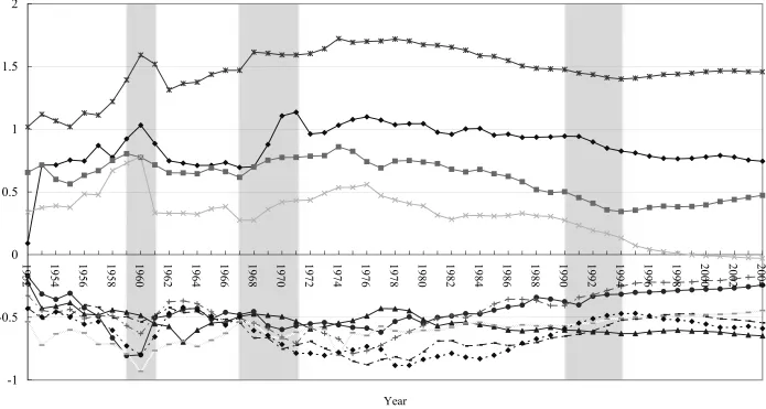
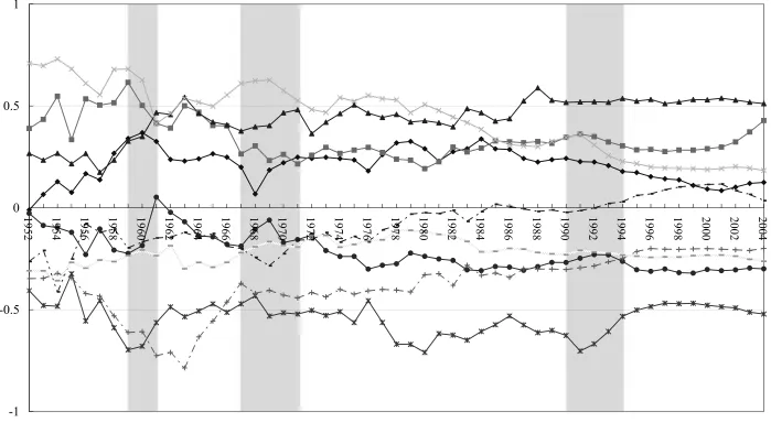
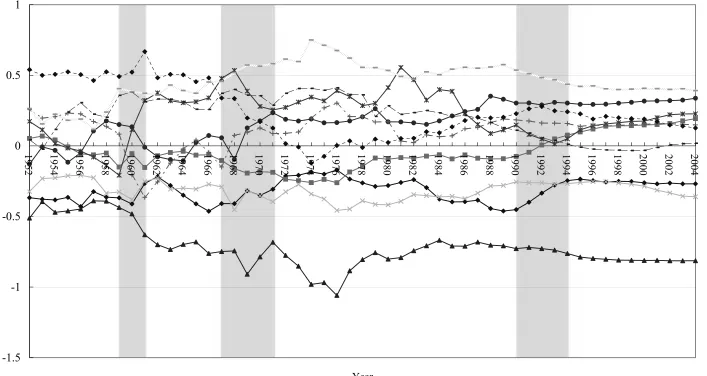
1978–1979; and Deng Xiaoping’s southern tour in 1992. Figures 1 to 3 show the

fluctuations of log of real per capita outputs of the provinces, wherein each series is

subtracted from the mean value of each of three regions, with twenty-nine provinces.4 5

In all the figures, we observe apparent shifts in the level of the series corresponding to

3

Carlino and Mills (1993), Greasley and Oxley (1997), and Li and Papell (1999) have

examined convergence using unit root tests which can deal with a breaking time series.

4

This classification of provinces is nearly identical to that of Zhang et al. (2001), but

the aggregation of provincial series is not conducted in this paper. The details will be

described in Section 4.1.

5

Studies on multi-country convergence often use the deviation from the cross-sectional

mean and look into its nonstationarity (Evans and Karras, 1996; Lee et al., 1997; and

each province for the following time periods: 1959–61, 1967–71, and the early 1990s

(shown as grey areas in the figures). These shifts coincide with the occurrences of the

events mentioned above. Based on these findings, some studies have focused on the

presence of structural changes in the annual series in China (Li, 2000; Zhang et al.,

2001; and Smyth and Inder, 2004); these studies have adopted unit root testing methods

permitting one or two breaks in a single time series for the analysis of the

nonstationarity of the macroeconomic or provincial time series.

However, with regard to the convergence hypothesis in regional panel data in

China, published papers which explicitly deal with the existence of multiple structural

breaks occurring at different break dates in the panels have been few in number.6

6

In general, existing panel-based unit root tests which allow for breaks may be too

restrictive for empirical applications based on the convergence hypothesis. Specifically,

these tests are based on two major assumptions: the presence of a linear time trend in a

series and the absence of cross-sectional dependence between error terms in the data

generating process (DGP). In the case of the former assumption, the tests defined under

the DGP with a time trend are not directly applicable to investigations on convergence.

In these investigations, the difference between two series or the deviation from the

mean value of all cross-sectional units is usually used, and the difference or the mean

deviation is often assumed to be zero mean stationary when absolute convergence exists,

or level stationary when conditional convergence exists (Bernard and Durlauf, 1995;

Evans and Karras, 1996). Thus, these analyses require tests which are defined under

Therefore, while examining convergence across provinces in China, this study focuses

on the presence of multiple structural breaks in the panels. Based on the combining

p-values method of Fisher (1932), we first develop a unit root test which allows for

multiple breaks in the panels. We then investigate the existence of regional convergence

in China by applying the test to China’s provincial per capita outputs. The p-values of

the t-type unit root tests for each province, which are combined by the panel unit root

tests based on Fisher’s p-values combination approach, are calculated by Monte Carlo

simulation under three data generating models—the driftless random walk model, the

ARMA model, and the AR model with cross-sectionally dependent errors. In particular,

in the case of cross-sectional dependence between error terms, the bootstrap method

proposed by Maddala and Wu (1999) and Wu and Wu (2001) is employed in order to

correct the biases of the panel-based unit root tests.7

The remaining sections of this paper are organized as follows: Section 2 defines

convergence; Section 3 describes the econometric methodology; Section 4 briefly

mentions the data and discusses the empirical results; and Section 5 presents the

conclusions.

assumption, cross-sectional correlation between error terms is a major issue in dynamic

panel estimation because neglecting this correlation may lead to a bias of an estimated

parameter and increase its variance (O’connell, 1998; Phillips and Sul, 2003).

7

Banerjee and Carrion-i-Silvestre (2006) have dealt with several issues on structural

2. Definition of Convergence

At first, we consider convergence as proposed by Evans (1998). Suppose that y_it is a

log per capita output for province (cross-sectional unit) i at time t (i=1,K,N ,

T

t =1,K, ). Next, consider the difference between y_it and the mean value of y_it

over i=1,K,N , which is denoted as y%_it≡ y_it−y_t, where 1

1

N it

t N i y

y ≡ −

∑

by Evans (1998), since 1

1( )

N

it t j it jt

y −y =N−

∑

pairs of i and j, y_it−y_t is stationary for all i. A converse proof is also available:

since y_it −y_jt =(y_it −y_t) (− y_jt−y_t), if y_it−y_t is stationary for all i, y_it −y_jt is

stationary for all pairs (i, j). These results equate bivariate convergence within all

pairs of provinces, reflected by the stationarity of y_it−y_jt for all pairs of i and j, to

the stationarity of y_it−y_t for all i. This equivalence enables us to focus on

investigating the stochastic properties of y%it= yit−yt for all i instead of yit−yjt

for all pairs of i and j.

In the next section, we will specify structural changes at some time periods in a

series as multiple shifts in the level of the series. Accordingly, convergence is defined

as follows:

For all i , if y%_it is stationary with shifts in its level at some t , then convergence exists

across all the provinces.8

8

Evans and Karras (1996) have postulated that convergence is absolute if y%_it has a

zero mean for all i, or conditional if y%_it has a non-zero mean for some i. According

to Evans and Karras, when all the series of y%_it are stationary and have some structural

This study does not allow the trend stationarity of y%_it for each i because the

presence of a linear time trend implies that some of the differences between y_it and

jt

y for fixed i and all j will diverge as time approaches infinity unless the time

trends are the same for all the pairs (Bernard and Durlauf, 1995). Further, with the

exceptions of Liaoning in Figure 1 and Heilongjiang and Hubei in Figure 2, none of the

figures show a distinct upward or downward tendency for any series during the entire

sample period. Therefore, we consider y%_it as a series without a time trend in the later

sections.

3. Econometric Methodology

3.1. Models and Test Statistics for a Single Time Series

We assume y%_it for each province to be nonstationary without breaks under the null

hypothesis, and stationary with breaks under the alternative hypothesis. As discussed in

Section 2, although each series exhibits no linear time trend, it contains some shifts in

the level. Therefore, this study assumes that y%_it is generated by the following data

generating process (DGP).

Under Null ~y_it = ~y_it−1 +ε_it (1) Under Alternative ~y_it =ρ_i~y_it−1+δ_1iDU_1it +δ_2iDU_2it +ε_it, ρ_i <1 (2)

N

i=1,K, , t =1,K,T

i after the last break date, or conditional if y%_it has a non-zero mean for some i after

where ε_it is independently and identically distributed across i and t with a zero

mean and a finite variance; δ_hi denotes the size of the hth break (h=1, 2); DU_hit

denotes the hth break in the level of a series (h=1, 2), where DU_hit =1 for t >τ_hiT,

and zero otherwise; and τ_hi is the fraction of the h th break ( h=1, 2) in

1

0<τ_1i <τ_2i < , which is defined as TB_hi /T for all T, where TB_hi is the date of the

hth break (h=1, 2). In this DGP, the series is a driftless random walk process under

the null hypothesis, whereas it is a stationary process and has up to two-time level shifts

under the alternative hypothesis. Next, the regression model nests Models (1) and (2).

error DU

DU y

d

y_it = _{mi m}+ _{i it} + _{i it} + _{i it} +

∆~ _{αˆ φ}ˆ~ _{−1 δ}ˆ_{1 1 δ}ˆ_{2 2 m=1, 2 (3)}

where ∆~y_it =~y_it −~y_it−1, φˆ_i = ρˆ_i −1, and d_m denotes the deterministic term, where

{ } m

d = ∅ for m=1 and {1} for m=2. Let t_im be the t-statistic testing the null

hypothesis φˆ_i =0 and δˆ_1i =δˆ_2i =0 against the alternative hypothesis φˆ_i ≠0 and

0 ˆ

1i ≠

δ , δˆ_2i ≠0 in each regression model m (m=1, 2) for each i. As carried out in

Zivot and Andrews (1992) and Lumsdane and Papell (1997), the break dates

} ,

{TB_1i TB_2i are endogenously determined to be where the one-sided t_im-statistic is

minimized in sequential estimations over all possible break dates within the range of

1

0<τ_1i <τ_2i < . For fixed i, when Model (1) has a constant and Model (3) has both a

constant and linear time trend, the t_im-statistic is the counterpart of the one proposed by

Zivot and Andrews (1992) for a single break (δ_2i =0 and δˆ_2i =0) and of that

proposed by Lumsdane and Papell (1997) for double breaks, where the asymptotic

behaviour of the statistic as T →∞ can be found. On the other hand, no literature

provides the exact asymptotic behaviour of the test considered here. Therefore, as

∞ →

breaks in the following theorems in which the subscript i is omitted for simplicity.

Theorem 1.For Models (1) and (3), with δ₂ =0 and δˆ₂ =0, as T →∞, the limiting distribution of the minimum t -statistic is given as follows: m

(

)

{

}

  +

⇒

_∫

_∫

0 1 2 / 1 1 0 2 1 2

1) inf 1 ( , ) ( , )

(

1 m m m m

m dW r W dr r W b

t τ τ τ

τ m=1, 2 (4)

where ⇒ denotes weak convergence in distribution; W_m(r,τ₁) denotes the residuals

from the projection of a standard Wiener process W(r) onto the subspace generated

by the functions

{

}

{

}

1 ) , ( ₁ 1 r τ =

du for r >τ₁, and zero otherwise. b is given by_m

{

}

b = − −1

∫

{

}

∫

1 ) ( ) 1 ( τ µ τ τ

where Wµ(r) is a demeaned standard Wiener process defined as

) ( )

(r W r

Wµ ≡ −

∫

The proof of Theorem 1 is analogous to the following theorem and is, therefore,

omitted.9

Theorem 2. For Models (1) and (3), as T →∞, the limiting distribution of the minimum t -statistic is given as follows: _im

(

)

{

}



 _{+ +}

⇒ _{m m}

∫

∫

m dW r W dr r W c b t 1

0 1 2

2 / 1 1 0 2 2 1 2 2 , 2

1, ) inf 1 ( , , ) ( , , )

( 2 1 τ τ τ τ τ τ τ

τ m=1, 2 (5)

9

where W_m(r,τ₁,τ₂) denotes the residuals from the projection of W(r) onto the

subspace generated by the functions

{

}

{

}

otherwise (h=1, 2). b and _m c are given by_m

{

}

∫

∫

2 1 ) ( ) ( ) ( τ τ τ τ

{

}

c₁ = ₂ − ₁ −1 −

∫

∫

τ τ τ

τ τ

{

}

b = − − − −

∫

∫

0 0 2 1 1 1 1 2

2 ( ) ( ) ( )

τ _µ τ _µ τ τ τ τ

{

}

c = − −

∫

∫

0 1 2 1 0 1 1 2

2 ( ) ( ) (1 )(1 ) ( )

τ _µ τ _µ τ τ τ τ .

The proof of Theorem 2 is given in Appendix.

3.2. Construction of Panel Unit Root Test with Breaks

In this subsection, we construct a panel unit root test with breaks by combining the

individual minimum t_im-test; this test is based on Fisher’s (1932) sum of log p-value

approach, which has been introduced and used by Maddala and Wu (1999).

Suppose that p_i is the p-value from the ith test statistic among N continuous

test statistics. Therefore, since each p_i is an independent uniform (0, 1) variable,

i

p

log 2

− has the chi-square distribution with two degrees of freedom. Further, the

summation of −2logp_i from i=1 to N also has the chi-square distribution with

N

2 degrees of freedom. Fisher (1932) utilized this fact to develop the test (hereafter,

Fisher test). By applying Fisher’s p-value combination method to N augmented

Dickey–Fuller t-tests, Maddala and Wu (1999) has built a panel-based unit root test

which does not allow breaks. In this study, we use Fisher’s approach to construct panel

individual minimum t_im-test. Therefore, the sum of logp_im is defined as follows:

∑

−

= N

i

m i

p B

Fisher

1

log 2

_ m=1,2 (6)

The Fisher_B test (the Fisher test with breaks) also has the chi-square distribution with

N

2 degrees of freedom. In the present case, however, the degree of freedom of the

chi-square distribution is 2(N −1) due to the restriction of ~ 0

1 =

∑

N

i yit . The null and

alternative hypotheses of the test are specified as H₀: 0φ_i = and δ_1i =δ_2i =0 for

all i and H₁: 0φ_i < and δ_1i ≠0, 0δ_2i ≠ for some i respectively.

There are two noteworthy features of the tests based on Fisher’s p-value

combination approach: (1) Since the tests have an exact (chi-square) distribution, they

do not require a large cross-sectional dimension of panel data. Hence, they are expected

to perform well in the analyses using panels with a relatively large time dimension and a

small cross-sectional dimension such as country-level, state-level, or provincial-level

panels.10 (2) Even if some of the N unit root tests give larger p-values than

conventional significance levels, e.g. 5 or 10 per cent, which implies the non-rejection

of the unit root null in each test, if these p-values indicate a slight tendency to reject the

unit root null (e.g. 0.15 or 0.2), the tests based on Fisher’s p-value combination

approach can capture it.

To calculate the Fisher_B test statistic, we need to compute the p-value of the

10

Although Becker (1997) compared the performance of 16 p-value combination tests,

including the Fisher test, he concluded that there was no test that was the most accurate

minimum t_im-test for all (i, m) by Monte Carlo simulation because the minimum

m i

t -test has non-standard limiting distributions for each m shown in Theorems 1 and 2.

Under the unit root null hypothesis, this study considers the following three DGPs:

Model (I) ~y_it = ~y_it−1 +ε_it

Model (II) θˆ_i(L)∆~y_it =ψˆ_i(L)σˆ_iε_it

Model (III) *

1 *

* _ˆ ~

~ it k k k it ik it i y

y = γ ∆ +ε

∆

∑

= −

where ε_it is an i.i.d. N(0, 1) error across i and t ;

= ) ( ˆ _L

i

θ − − 2 −

2 1 ˆ ˆ

1 θ _iL θ _iL i i p i p L θˆ −

L and ψˆ_i(L)=1−ψˆ_1iL−ψˆ_2iL2 − i

i q i q L ψˆ −

L , where

p

θ θˆ_{, ,} ˆ

1 L and ψˆ1,L,ψˆq are estimated parameters; and L is the lag operator such as

1 −

= _t

t y

Ly . For Model (I), ~ is generated for each y_it i by a driftless random walk

model. For Model (II), for each i, ∆y~_it is generated by the optimal autoregressive

moving average (ARMA) (p_i, q_i) model with estimated parameters and N(0, σˆ_i2)

innovations, where σˆ_i2 is the estimated innovation variance of the ARMA model. The

selection of the optimal ARMA model follows the Zivot and Andrews (1992) procedure,

which fits ARMA(p, q) model to ∆~y_t over the possible combinations of p and q

with 5p, q≤ , then finds the best fitted model according to the Akaike information

criterion and the Schwartz information criterion. When the two criteria choose different

models, the most parsimonious model is selected.

For Model (III), ∆~y_it* is the bootstrap sample for ∆~y_it, which is obtained by the

bootstrap method employed by Maddala and Wu (1999) and Wu and Wu (2001). The

procedure followed herein is elaborated below. Firstly, we estimate the equation

0 1 ~ ˆ ~ it k

k ik it k

it

i

y

y = γ ∆ +ε

residuals ε_t0 =[ε₁0_t,ε₂0_t,L,ε_Nt0 ] (t =1,K,T ). Next, we resample ε_it0 from the obtained

residuals by preserving their cross-sectional correlation structure based on the bootstrap

method of Maddala and Wu (1999), wherein the vector ε_t0 =[ε₁0_t,L,ε_Nt0 ] is resampled

instead of individual ε_it0. In addition, we generate a random number g which takes

integer values on [1, T] with probability 1/T, by using a uniform random number.

We then draw a row of residuals 0 =

g

ε [ 0 0

1g, ,εNg

ε L ] according to the realizations of g.

The bootstrap sample ε_t* (t =1,K,T ) is obtained by T-time withdrawals from the

residuals. The bootstrap sample ~y_it* is generated by Model (III) with estimated

parameters γˆ (_ik k =1,K,k_i) in the previous OLS estimation. However, *

1 *

1

~ , , ~

+ i

k i

i y

y L

are replaced by the sample obtained by the block resampling method of Berkowitz and

Kilian (1996). Their method divides the actual sample y~ into _it T −k_i overlapping

subsampling blocks with size k_i +1 and randomly draws a block from T −k_i blocks.

Then, *

1 *

1

~ , , ~

+ i

k i

i y

y L are replaced with this block.

In fact, in the case where the cross-sectionally dependent errors are present in the

data generating model, the Fisher_B test does not belong to the chi-square distribution

under the null hypothesis because the minimum m

i

t -tests are correlated across i.

Accordingly, the test may be biased towards over- or under-rejections of the null.

In order to correct these biases of the test, we first capture the cross-sectional

correlation structure in the panels according to the above resampling scheme.11 Then,

with the generated bootstrap sample ~y_it* (t =1,K,T ), we obtain the empirical

11

To remove cross-sectional dependence in the panels with structural breaks, the

distribution function of the Fisher_B test through simulation, which provides the

appropriate small-sample critical values for the test. These values are listed in Table 2.

Based on these simulated critical values, we can conduct unit root testing in an

appropriate manner.

A Monte Carlo simulation is performed using 5,000 replications under each DGP.

The summary of the simulation is as follows:

(1) For each i, the empirical distribution function of the minimum t_im-statistic is

obtained through replications. In particular, in Model (III), 5,000 bootstrap samples

are generated and used in the simulation.

(2) For each i, the p-value ( m

i

p ) of the actual minimum m

i

t -test, obtained from the

original data set, is evaluated based on the empirical distribution function obtained

in (1). Then, the Fisher_B statistic is calculated.

(3) In each replication in Model (III), p_im of the simulated minimum t_im-test, which

is computed from each bootstrap sample, is evaluated for each i based on the

empirical distribution function obtained in (1). Then, using p₁m,K,p_Nm, the value

of −

∑

i

m i p

1log

2 is calculated. The empirical distribution function of the

Fisher_B test can be obtained from the calculated values of −

∑

i p

log

2 .

4. Empirical Analysis

4.1. Data

Provincial data have been sourced from China Compendium of Statistics 1949–2004.

these outputs have been generated by the chain index of the per capita gross regional

product (GRP) with 1952 as the reference year.12 Hainan and Sichuan provinces have

been excluded due to the lack of data. All the series used in this paper have been taken

in natural logarithms.13

As in Zhang et al. (2001), we divide the 29 provinces according to their

geographical locations into the following three regions: the Eastern, Central and

Western regions.14 However, we have included the Guangxi Zhuang autonomous

12

The chain index of the per capita GRP is computed as

) 100 / ( ) 100 / ( ) 100 / (

100 _{52 53}

*

t

t Y Y Y

Y = ⋅ ⋅ L , where Y_t* is the chain index of the per

capita GRP. Further, Y_t is the index of the per capita GRP (preceding year = 100), and

52

Y is set to 100.

13

The quality of official Chinese statistics has been argued by many researchers (e.g.

Chow, 1986; Rawski, 2001; and Holz, 2006). Currently, it is widely recognized that

official Chinese data at the national and provincial levels have certain inconsistencies

and miscalculations due to factors such as the lack of technical personnel for the

collection of statistics and political pressure to exaggerate statistics at the lower levels.

However, our results, which will be presented in Section 4.3, remain valid as long as the

stochastic properties of the series used in this paper do not change even if there are

certain inaccuracies in them.

14

The Eastern region has the following ten provinces: Beijing, Tianjin, Hebei,

Liaoning, Shanghai, Jiangsu, Zhejiang, Shandong, Fujian, and Guangdong. The Central

region in the Western region, instead of the Eastern region, because since 1978, its log

of real per capita output has shown considerable deviation from those of the other

Eastern provinces. In fact, the differences between the recent data of Guangxi and other

Western provinces are considerably less compared to the differences between Guangxi

and other Eastern provinces. Therefore, it is reasonable to include Guangxi in the

Western region.15

The panel for each region used in this study is composed of the deviations of a log

of real per capita output from the mean value across all the provinces in the

corresponding region, which is denoted by N _{it t}

i it it

it y y y y

y = −

∑

1

~ _{, where} '

N is

the number of provinces in the region.

4.2. Test Procedure

Model (3) shown in Section 3.1 is regressed for each m , including lagged

augmentation terms of the first difference of ~ , in order to eliminate the y_it

Heilongjiang, Anhui, Jiangxi, Henan, Hubei, and Hunan. The Western region consists

of the following ten provinces: Guangxi, Chongqing, Guizhou, Yunnan, Tibet, Shaanxi,

Gansu, Qinghai, Ningxia, and Xinjiang.

15

For example, for the series (in logarithms) in 2004, the difference between the series

of Guangxi and Hebei (the closest series among other Eastern provinces) is 0.87. In

contrast, the difference between the series of Guangxi and Yunnan (the closest among

the Western provinces) is 0.09. In addition, the series of some other provinces in the

autocorrelation of the error term.

it l

l

l it il it

i it i it i m mi

it d y DU DU a y u

y

i

+ ∆ +

+ +

+ =

∆

∑

= −

−

1 2 2 1 1 1

~ ˆ ˆ

ˆ ~ ˆ ˆ

~ _{α φ δ δ (7)}

where l_i is a lag order parameter and u_it is a serially uncorrelated error. We

determine the number of lagged augmentation terms by following the

‘general-to-specific’ procedure described in Perron (1989) and suggested in Ng and

Perron (1995). The maximum lag order is set at 8. Next, the procedure first estimates

the regression model with l_i =8. If the last lag is significant at 10 per cent, where the

critical value is an asymptotic normal value of 1.645 on the t-statistic, the procedure

selects 8 as the optimal lag order; otherwise, it is eliminated from the regression model.

The steps mentioned above are repeated until the last lag becomes significant. In the

event of a single insignificant lag, the optimal lag order is set at 0.

For each i, the minimum t_im-test statistic is obtained by sequentially regressing

Model m ( m=1, 2 ) over the possible break dates {TB_1i, TB_2i} within

53

1+l_i <TB_1i <TB_2i < for two-time breaks and {TB_1i} within 1+l_i <TB_1i <53 for

a one-time break. Then, for each of the three regions, the Fisher_B test is constructed

for each m (m=1, 2) by combining the p-value of the individual test ( p_im), which is

obtained via simulation.

4.3. Test Results and Discussion

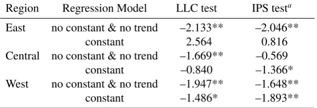
We first employ the commonly used panel unit root tests without a break—the Levin,

Lin and Chu (2002) test and the Im et al. (2003) test. The results are shown in Table 1.

regression model at the 10 per cent or better significance level. From this test result, the

convergence hypothesis of the provincial outputs appears to be supported for each

region. However, the IPS and LLC tests may possibly suffer from biases towards under-

or over-rejections of the unit root null because they do not treat the presence of both

structural breaks and cross-sectional dependence among error terms in the panels.16

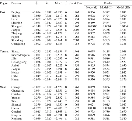
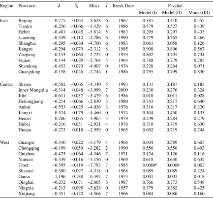
Next, we apply the tests based on Fisher’s p-value combination approach—the

MW test and the Fisher_B test—on series with breaks (The estimation results for each

province in the presence of breaks are presented in Tables 1A–4A in Appendix.).17

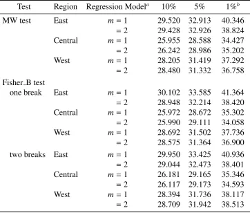
Table 2 provides the small-sample critical values at the 10, 5, and 1 per cent levels of

the MW and Fisher_B tests under Model (III), which are obtained by using the

procedure described in Section 3.2.

Table 3 reports the test results obtained under the three DGPs. In the case of tests

on series without a break (the MW test), there are ten significant tests of regional

16

With regard to these issues, Perron (1989), Leybourne et al. (1998), and Im et al.

(2005) have revealed that ignoring breaks in a single time series or panel data can lead

to an erroneous inference in a test, while O’connell (1998) and Phillips and Sul (2003)

have argued that estimated parameters tend to be biased by the presence of

cross-sectionally correlated errors.

17

We have also obtained test results for cases in which the mean deviations of log per

capita outputs display a linear time trend for Liaoning in the Eastern region and

Heilongjiang and Hubei in the Central region. Since these results are quite similar to

convergence of real per capita outputs. In these tests, however, due to the omission of

breaks, the test results might be inaccurate and, therefore, misleading.

We then consider the possibility of structural breaks occurring at various break

dates across provinces. The fourth column of Table 3 shows the results of the Fisher_B

test in the case of a one-time break. When Models (I) and (II) are used as DGPs, for the

Western region, the Fisher_B test rejects the unit root null hypothesis for both the

regression models (m=1, 2) at the 1 per cent significance level. In addition, under both

the DGPs, significant rejections of the null are observed at the 10 per cent level for the

Eastern region (m=1) and at the 10 or 5 per cent level for the Central region (m=2).

In the case of Model (III), wherein there is the cross-sectional correlation between error

terms, the test statistics for both the regression models for the Western region are still

higher than the corresponding critical values at the 1 per cent significance level. Further,

the statistic of the regression model for the Eastern region where m=1 is also

significant at the 10 per cent level. In the case of Central provinces, the Fisher_B test

cannot support the stationarity alternative. In Model (III), the finding that convergence

occurs within all provinces in the Eastern and Western regions appears to be consistent

with that of Zhang et al. (2001).

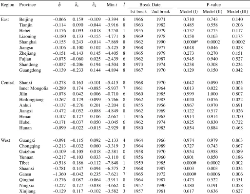
The last column of Table 3 presents the results for cases with two-time breaks. In

Models (I) and (II), with one exception in the Central region, all the test results for all

the regions exhibit significant rejections of the unit root null hypothesis at the 5 per cent

or better levels. Moreover, when the correlation of error terms among provinces in each

region is considered in Model (III), the Fisher_B test also strongly supports the

the regression models). As compared to the case of a series that includes a single

structural break, under any DGP, this case indicates the existence of regional

convergence within all the three regions. Therefore, it should be concluded that dealing

with multiple structural breaks occurring at different break dates for each province

provides stronger evidence of the existence of convergence within regions in China.

This fact may also account for the discrepancies in the results compared with those of

Zhang et al. (2001), where one endogenous break point is assumed in their estimation.

The comparison of the three tests results shown in Table 3 reveals that they greatly

depend on the number of breaks allowed in the tests. As discussed in Section 1, due to

the impact of certain significant political and economic events, the provincial real per

capita outputs in China are suspected to have some structural breaks; therefore, in the

analysis on regional convergence in China, we consider it appropriate to examine the

possibility of multiple structural changes in the studied time periods. Consequently,

when the provincial log per capita outputs are allowed to have two-time level shifts at

various break dates across the provinces, we observe convergence of the series in all the

three regions.

4.4. Test Results Based on Other Regional Classifications 18

As illustrated in Figure 1, the mean deviation of the real per capita output for

Shanghai is much larger than those for other Eastern provinces. Since this may be

indicative of the heterogeneity of Shanghai, the series for nine Eastern provinces,

18

excluding Shanghai, have been tested. Consequently, convergence is also observed in

the Eastern region.

Further investigations have been conducted based on other data classifications

where the Eastern region (with or without Shanghai) includes the neighboring provinces,

which are Guangxi, Jilin, and Heilongjiang. The cases where one, two, or all of the

provinces are classified as belonging to the Eastern region are analyzed. As a result, in

the case of two structural breaks, the evidence of convergence has been found in all the

classifications. This fact seems to imply that the neighboring provinces are on the same

path of convergence as that of other Eastern provinces; however, this is not

conclusive.19

To make the discussion more concrete, in classifying provinces into certain regions,

the use of classification methods such as cluster analysis would be desirable. The work

of Hobijn and Franses (2000) is one such application. However, this is beyond the scope

of this paper. Meanwhile, as discussed in Section 4.1, there appear to be substantial

grounds for our classification of Chinese provinces. Therefore, our findings obtained

from Table 3 are meaningful.

19

In addition, the sample consisting of whole provinces has been tested; moreover, a

significant rejection of the unit root null hypothesis has been obtained. However, we

believe that further information (e.g. the homogeneity of provinces classified into

5. Conclusion

In this study, we investigated the regional convergence hypothesis of the provincial per

capita outputs in China while considering up to two-time structural breaks in the panels.

According to the p-value combination approach of Fisher (1932), the panel-based unit

root test has been developed by combining the p-value of the individual unit root test

which allows for breaks in a single time series. This approach allowed us to consider

multiple breaks at various break dates across the provinces. We used three data

generating models in the Monte Carlo simulation—the driftless random walk model, the

ARMA model, and the AR model with cross-sectionally dependent errors—to calculate

the p-value of the individual minimum t-type unit root test from its empirical

distribution. In particular, in the case of the AR model with cross-sectionally dependent

errors, the empirical distribution of the test for each province was generated on the

bootstrap samples, which were obtained by the resampling procedure proposed by

Maddala and Wu (1999) and Wu and Wu (2001). On the basis of their geographical

locations, the provinces were grouped into the following three regions: the Eastern,

Central, and Western regions. Subsequently, the existence of convergence within each

region was tested by the panel unit root test with breaks, which was developed in this

paper. As a result, when the presence of two-time breaks was considered in the test, we

found significant evidence to suggest that the convergence of the provincial per capita

outputs exists within each region.

Acknowledgement

participants at Yokohama Symposia in 2007 for their helpful comments.

References

Banerjee, A. and Carrion-i-Silvestre, J. L. (2006) Cointegration in panel data with

breaks and cross-section dependence, EUI Working Papers, ECO No. 2006/5, 1-47.

Barro, R. J. (1991) Economic growth in a cross section of countries, The Quarterly

Journal of Economics, 106, 407-443.

Barro, R. J. and Sala-i-Martin, X. (1992) Convergence, Journal of Political Economy,

100, 223-251.

Becker, B. J. (1997) P-values, combination of, in Encyclopedia of Statistical Sciences:

Update vol.1 (Ed.) S. Kotz and N. L. Johnson, Wiley, New York, pp.448-453.

Berkowitz, J. and Kilian, L. (1996) Recent developments in bootstrapping time series,

Discussion paper 96/54, Board of Governors of the Federal Reserve System.

Bernard, A. B. and Durlauf, S. N. (1995) Convergence in international output, Journal

of Applied Econometrics, 10, 97-108.

Bernard, A. B. and Durlauf, S. N. (1996) Interpreting tests of the convergence

hypothesis, Journal of Econometrics, 71, 161-173.

Carlino, G. A. and Mills, L. O. (1993) Are U.S. regional incomes converging? A time

series analysis, Journal of Monetary Economics, 32, 335-346.

Chen, J. and Fleisher, B. M. (1996) Regional income inequality and economic growth in

China, Journal of Comparative Economics, 22, 141-164.

Chow, G. C. (1986) Chinese statistics, The American Statistician, 40, 191-196.

Review, 39, 295-306.

Evans, P. and Karras, G. (1996) Convergence revisited, Journal of Monetary Economics,

37, 249-265.

Fisher, R. A. (1932) Statistical Methods for Research Workers, Oliver & Boyd,

Edinburgh, 4th Edition.

Fleissig, A. and Strauss, J. (2001) Panel unit-root tests of OECD stochastic convergence,

Review of International Economics, 9, 153-162.

Greasley, D. and Oxley, L. (1997) Time-series based tests of the convergence

hypothesis: some positive results, Economics Letters, 56, 143-147.

Gundlach, E. (1997) Regional convergence of output per worker in China: a

neoclassical interpretation, Asian Economic Journal, 11, 423-442.

Hobijn, B. and Franses, P. H. (2000) Asymptotically perfect and relative convergence of

productivity, Journal of Applied Econometrics, 15, 59-81.

Holz, C. A. (2006) Why China’s new GDP data matters, Far Eastern Economic Review,

169, 54-57.

Im, K.-S., Lee, J. and Tieslau, M. (2005) Panel LM unit-root tests with level shifts,

Oxford Bulletin of Economics and Statistics, 67, 393-419.

Im, K.-S., Pesaran, H. and Shin, Y. (2003) Testing for unit roots in heterogeneous

panels, Journal of Econometrics, 115, 53-74.

Jian, T., Sachs, J. D. and Warner, A. M. (1996) Trends in regional inequality in China,

China Economic Review, 7, 1-21.

Lee, K., Pesaran, M. H. and Smith, R. (1997) Growth and convergence in a

12, 357-392.

Levin, A., Lin, C.-F. and Chu, C. (2002) Unit root test in panel data: Asymptotic and

finite sample results, Journal of Econometrics, 108, 1-24.

Leybourne, S. J., Mills, T. C. and Newbold, P. (1998) Spurious rejection by

Dickey–Fuller tests in the presence of a break under the null, Journal of

Econometrics, 87, 191-203.

Li, Q. and Papell, D. (1999) Convergence of international output: Time series evidence

for 16 OECD countries, International Review of Economics and Finance, 8, 267-280.

Li, X.-M. (2000) The Great Leap Forward, economic reforms, and the unit root

hypothesis: testing for breaking trend functions in China’s GDP data, Journal of

Comparative Economics, 28, 814-827.

Lim, L. K. and McAleer, M. (2004) Convergence and catching up in ASEAN: a

comparative analysis, Applied Economics, 36, 137-153.

Lumsdaine, R. L. and Papell, D. H. (1997) Multiple trend breaks and the unit-root

hypothesis, The Review of Economics and Statistics, 79, 212-218.

Maddala, G. S. and Wu, S. (1999) A comparative study of unit root tests with panel data

and a new simple test, Oxford Bulletin of Economics and Statistics, 61, 631-652.

Mankiw, N. G., Romer, D. and Weil, D. N. (1992) A contribution to the empirics of

economic growth, The Quarterly Journal of Economics, 107, 407-437.

McCoskey, S. K. (2002) Convergence in Sub-Saharan Africa: a nonstationary panel

data approach, Applied Economics, 34, 819-829.

National Bureau of Statistics (2005) China Compendium of Statistics 1949–2004, China

Ng, S. and Perron, P. (1995) Unit root tests in ARMA models with data-dependent

methods for the selection of the truncation lag, Journal of American Statistical

Association, 90, 268-281.

O’connell, P. G. J. (1998) The overvaluation of purchasing power parity, Journal of

International Economics, 44, 1-19.

Oxley, L. and Greasley, D. (1995) A time-series perspective on convergence: Australia,

UK and USA since 1870, The Economic Record, 71, 259-270.

Pedroni, P. and Yao, J. Y. (2006) Regional income divergence in China, Journal of

Asian Economics, 17, 294-315.

Perron, P. (1989) The great crash, the oil price shock, and the unit root hypothesis,

Econometrica, 57, 1361-1401.

Perron, P. (1994) Trend, unit root and structural change in macroeconomic time series,

in Cointegration for the applied economists, (Ed.) B. B. Rao, Macmillan, Basingstoke

pp.113-146.

Pesaran, M. H. (2004) A pair-wise approach to testing for output and growth

convergence, Mimeo, University of Cambridge.

Phillips, P. C. B. and Sul, D. (2003) Dynamic panel estimation and homogeneity testing

under cross section dependence, Econometrics Journal, 6, 217-259.

Quah, D. (1993a) Empirical cross-section dynamics in economic growth, European

Economic Review, 37, 426-434.

Quah, D. (1993b) Galton’s fallacy and tests of the convergence hypothesis, The

Scandinavian Journal of Economics, 95, 427-443.

Review, 40, 1353-1375.

Raiser, M. (1998) Subsidising inequality: Economic reforms, fiscal transfers and

convergence across Chinese provinces, Journal of Development Studies, 34, 1-26.

Rawski, T. G. (2001) What is happening to China’s GDP statistics? China Economic

Review, 12, 347-354.

Smyth, R. and Inder, B. (2004) Is Chinese provincial real GDP per capita

nonstationary? Evidence from multiple trend break unit, China Economic Review, 15,

1-24.

Weeks, M. and Yao, J. Y. (2003) Provincial conditional income convergence in China,

1953-1997: a panel data approach, Econometric Reviews, 22, 59-77.

Wu, J.-L. and Wu, S. (2001) Is purchasing power parity overvalued? Journal of Money,

Credit, and Banking, 33, 804-812.

Zhang, Z., Liu, A. and Yao, S. (2001) Convergence of China’s regional incomes

1952-1997, China Economic Review, 12, 243-258.

Zivot, E. and Andrews, D. W. K. (1992) Further evidence on the great crash, the

oil-price shock, and the unit-root hypothesis Journal of Business & Economic

Figure 1. Mean deviations of log of provincial real per capita outputs for the Eastern provinces

-1 -0.5 0 0.5 1 1.5 2

1952 1954 1956 1958 1960 1962 1964 1966 1968 1970 1972 1974 1976 1978 1980 1982 1984 1986 1988 1990 1992 1994 1996 1998 2000 2002 2004

Year

Beijing Tianjin Hebei Liaoning Shanghai Jiangsu

Figure 2. Mean deviations of log of provincial real per capita outputs for the Central provinces

-1 -0.5 0 0.5 1

1952 1954 1956 1958 1960 1962 1964 1966 1968 1970 1972 1974 1976 1978 1980 1982 1984 1986 1988 1990 1992 1994 1996 1998 2000 2002 2004

Year

Figure 3. Mean deviations of log of provincial real per capita outputs for the Western provinces

-1.5 -1 -0.5 0 0.5 1

1952 1954 1956 1958 1960 1962 1964 1966 1968 1970 1972 1974 1976 1978 1980 1982 1984 1986 1988 1990 1992 1994 1996 1998 2000 2002 2004

Year

Guangxi Chongqing Guizhou Yunnan Tibet Shaanxi Gansu

Table 1. The results for the Levin et al. (2002) (LLC) test and the Im et al. (2003) (IPS) test

Region Regression Model LLC test IPS testa East no constant & no trend –2.133** –2.046**

constant 2.564 0.816

Central no constant & no trend –1.669** –0.569 constant –0.840 –1.366* West no constant & no trend –1.947** –1.648**

constant –1.486* –1.893**

***, **, and * denote statistical significance at the 1%, 5%, and 10% levels, respectively.

a_{For both regression models, the means and the variances of the individual}

augmented Dickey–Fuller t-test forT =53−pi−1 were computed with 500,000

replications, wherepiis the number of lagged augmentation terms of the first

difference of a series added in the individual ADF equation.

Table 2. The critical values of the Maddala and Wu (1999) test and the Fisher B test in the case of cross-sectionally dependent errors

Test Region Regression Modela 10% 5% 1%b MW test East m= 1 29.520 32.913 40.346

= 2 29.428 32.926 38.824 Central m= 1 25.955 28.588 34.427

= 2 26.242 28.986 35.202 West m= 1 28.205 31.419 37.292

= 2 28.480 31.332 36.758 Fisher B test

one break East m= 1 30.102 33.585 41.364

= 2 28.948 32.214 38.420 Central m= 1 25.972 28.672 35.302

= 2 25.990 29.111 34.058 West m= 1 28.692 31.502 37.736

= 2 28.575 31.364 36.900 two breaks East m= 1 29.950 33.425 40.936

= 2 29.044 32.473 38.401 Central m= 1 26.181 29.165 35.346

= 2 26.117 29.173 34.593 West m= 1 28.394 31.736 38.117

= 2 28.709 31.942 38.513

a

The regression model is∆y˜it=αˆmidm+φˆiy˜it−1+δˆ1iDU1it+δˆ2iDU2it+P

¯

li

l=1aˆil∆y˜it−l+uit,

i = 1, . . . ,N′,t = 2, . . . ,53, whereN′ = 10 for the Eastern and Western regions and

N′=9 for the Central region, anddm={∅}form=1 anddm={1}form=2; in addition,

ˆ

δ1i=δˆ2i=0 for allifor the MW test and ˆδ2i=0 for allifor the Fisher B test for the one

break case.

b_{The values are 10, 5, and 1 per cent points on the right tail of the empirical distributions}

of the MW and Fisher B tests. These distributions are obtained as follows. For eachiand

m, under Model (III), the empirical distribution of the minimum tm

i-statistic is obtained

by a Monte Carlo simulation with 5,000 replications. Next, the percentage point (pm i)

of the minimumtm

i-statistic computed for each replication is evaluated on the empirical

distribution obtained in the first step. After this, the value of−2P_iN₌₁logpm

i is calculated

for each replication. The empirical distributions of the tests can thus be obtained from the calculated values of−2Plogpm

i.

Table 3. The results for the Maddala and Wu (1999) test and the Fisher B test in the cases of one-time and two-time breaks

Region Regression Modela _{MW test}b _{Fisher B test}b

(no break) one break two breaks

DGP Model (I): ˜yit =y˜it−1+ǫit

East m= 1 37.511*** 27.251#c_{* 39.156#***}

= 2 12.125 16.436 33.962**

Central m= 1 19.276 13.907 28.053**

= 2 25.340* 28.723** 41.961***

West m= 1 26.270* 37.805*** 52.676#***

= 2 26.751* 50.076#*** 58.674#***

DGP Model (II): ˆθi(L)∆y˜it =ψˆi(L) ˆσiǫit

East m= 1 35.940*** 26.638#* 37.975***

= 2 12.250 16.024 31.379**

Central m= 1 17.185 9.875 19.740

= 2 23.236 23.881* 36.547***

West m= 1 26.214* 38.109#*** 49.923***

= 2 27.492* 49.960#*** 58.591#***

DGP Model (III):∆y˜∗_it =P¯ki

k=1γˆik∆y˜

∗

it−k+ǫ

∗

it

East m= 1 19.601 31.744#* 53.414***

= 2 15.104 18.074 22.887

Central m= 1 17.042 23.211 36.035***

= 2 27.109* 24.817 29.930**

West m= 1 28.991* 41.450*** 45.013***

= 2 28.882* 37.688*** 34.546**

***, **, and * denote statistical significance at the 1%, 5%, and 10% levels, respectively.

a_{The regression model is∆y˜}

it = αˆmidm+φˆiy˜it−1+δˆ1iDU1it+δˆ2iDU2it+P

¯

li

l=1aˆil∆y˜it−l+uit,i =

1, . . . ,N′_{,t = 2, . . . ,53, whereN}′ _{= 10 for the Eastern and Western regions and N}′ _{= 9 for the} Central region, anddm={∅}form=1 anddm={1}form=2; in addition, ˆδ1i=δˆ2i=0 for allifor

the MW test and ˆδ2i=0 for allifor the Fisher B test for the one break case. b

Under Models (I) and (II), because of the restriction ofPNi=1y˜it=0, the degree of freedom of the

chi-square distribution of the test is 2(N−1).

c_{The sign # indicates that the p-values for some provinces were estimated to be zero due to the}

fact that for each of these provinces, the realization of the minimumtm

i -statistic lay far left from its

empirical distribution which was generated by a Monte Carlo simulation with 5,000 replications. Therefore, in order to calculate the Fisher B statistic, the obtained p-values for these provinces were assigned a value of 0.0002 (1/5000). This implies that we assume that the minimumtm

i -statistic for

each of these provinces took a value within the estimated empirical distribution only once in the 5,000 replications.

Appendix

Proof of Theorem

For simplicity, we omit the subscript i of a variable and denote a time series as merely

t

y instead of ~ used in the main text. Therefore, y_t y_t is assumed to be subject to

Models (1) and (2) with an i.i.d. innovation ε_t with a zero mean and a finite variance

2

σ . In this proof, we show the derivation only for the case of m=2 because that for

the case of m=1 is obtained along the same lines.

Let e_t be the OLS residual obtained by regressing y_t on an intercept and two

dummy variables (DU_1t and DU_2t) for t =1,K,T . Then, the residual is expressed as

(

) (

)

1 ˆ

ˆ _{DU DU DU DU}

S

e_t = _tµ −δ _t − −δ _t − (1A)

where S_tµ is the demeaned random walk process such as ≡ − −

∑

t t t

t S T S

S

1 1

µ

,

where =

∑

s s t

S

1ε , and h

T

t ht h DU

DU =

∑

1 ( h=1,2 ). Now, we write

µ 1 S X' X) (X'

δ_{ˆ =} −

, where δˆ =(δˆ₁,δˆ₂)' ; X=

(

)

(

)

1 h hT h

h DU , ,DU DU

DU − −

=

− _h L

h DU

DU ; µ =

(

)

S . Then, we have

(

)

∑

∑

∑

∑

∑

∑

1 1 2 1 1

1 2 1 1 1 1 2 1 1 2 / 3 1 2 2 / 1 ) 1 ( ) 1 ( ) ( 1 ˆ

τ _{µ µ} τ _µ

µ

τ _µ τ _µ

τ τ τ τ τ τ τ τ δ . Thus,       =           − − − + − − ⇒      

∫

∫

∫

∫

where ⇒ denotes weak convergence in distribution. Therefore,

(

)

(

)

2 / 1 1 1 1 2 / 1 2 / 1 2 /

1 _{ˆ ˆ}

DU DU T DU DU T S T e

T− _t = − _tµ − − δ _t − − − δ _t −

=σ

[

{

} {

}

]

where W₂(r,τ₁,τ₂) denotes the residual from the projection of W(r) onto the

subspace generated by the function

{

}

h

r>τ , and zero otherwise (h=1,2).

From the regression of e_t on e_t−1, we can obtain the t-test statistic as

(

)

2 2 1 2 2 1 1

∑

∑

t t t

e T s e e T

t (3A)

where = −

∑

t et et

T s 2 2 1 1 2 ) ˆ

( ρ , where ρˆ is the estimated coefficient of e_t−1 in the

regression of e_t on e_t−1. Now, we show the probability limits of −

∑

t et et

T 2 1 1 ,

∑

t et

T

2 2

1

2 _{and s}2_.

T−1

∑

{

}

1 1 2 1 1 2 1 1 _ˆ ) 1 ( ) 1 ( ˆ 1

1 τ τ τ δ

δ µ _τ

τ µ

µ _{∆ − + − + − + −}

= ∆ − ₊ = − − = − −

∑

∑

T _{T T T}

T t t t T t t t

{

}

1 2 1 2 2 1 2 1 2 2

1 _{ˆ ˆ}

) 1 ( ˆ ) 1 ( ) 1 ( ˆ 2

2 τ τ τ δ τ τ δδ

δ µ _τ

τ + −

− _{+ − + − + − + + −}

−T S _T y_T y _T y T .

Hence, we have the following limiting distribution.

{

}

∫

∫

∑

t ( ) ( ) ( ) 1 (1) (1 1) 1 0 1 0 2 2 1

1 σ µ µ τ τ

−B

{

∫

}

0 τ τ τ τ .

In the derivation above, we used the following facts that

∫

∑

(r dW r

W S S T T t t t µ µ µ µ _σ

, T 1/2S _T W ( _h)

h σ τ

µ µ τ ⇒ − ) 1 ( 2 /

1 _{y W}

T− _T ⇒σ , 1/2 ₁ ( )

h T W

y T

h σ τ

τ + ⇒

−