www.hydrol-earth-syst-sci.net/15/2763/2011/ doi:10.5194/hess-15-2763-2011
© Author(s) 2011. CC Attribution 3.0 License.
Earth System
Sciences
Interpolation of groundwater quality parameters with some values
below the detection limit
A. B´ardossy
Institute of Hydraulic Engineering, University of Stuttgart, Stuttgart 70569, Germany Received: 10 May 2011 – Published in Hydrol. Earth Syst. Sci. Discuss.: 26 May 2011 Revised: 19 August 2011 – Accepted: 22 August 2011 – Published: 1 September 2011
Abstract. For many environmental variables, measurements cannot deliver exact observation values as their concentra-tion is below the sensitivity of the measuring device (detec-tion limit). These observa(detec-tions provide useful informa(detec-tion but cannot be treated in the same manner as the other mea-surements. In this paper a methodology for the spatial inter-polation of these values is described. The method is based on spatial copulas. Here two copula models – the Gaussian and a non-Gaussian v-copula are used. First a mixed maximum likelihood approach is used to estimate the marginal distri-butions of the parameters. After removal of the marginal distributions the next step is the maximum likelihood esti-mation of the parameters of the spatial dependence including taking those values below the detection limit into account. Interpolation using copulas yields full conditional distribu-tions for the unobserved sites and can be used to estimate confidence intervals, and provides a good basis for spatial simulation. The methodology is demonstrated on three dif-ferent groundwater quality parameters, i.e. arsenic, chloride and deethylatrazin, measured at more than 2000 locations in South-West Germany. The chloride values are artificially censored at different levels in order to evaluate the proce-dures on a complete dataset by progressive decimation. In-terpolation results are evaluated using a cross validation ap-proach. The method is compared with ordinary kriging and indicator kriging. The uncertainty measures of the different approaches are also compared.
Correspondence to: A. B´ardossy
1 Introduction
There are many different chemicals which enter the ground-waterwater system through different mechanisms. Many of these compounds are known or suspected to have adverse ef-fects on health and environment. Recent advances in labo-ratory techniques are providing improved capabilities for de-tecting large numbers of new and potentially harmful con-taminants. The concentrations of different chemicals usu-ally have strongly skewed distributions with a few very high values and a large number of low ones. Some of the low values are reported as non-detects due to the limited sen-sitivity of the laboratory instruments. The high skew and the occurrence of non-detects interpreted as values below a given threshold make the statistical and geostatistical anal-ysis of these data unpleasant and complicated. The statisti-cal treatment of censored data has a long history. Already Cohen (1959) had published a paper for the estimation of the normal distribution from censored data. Later work was per-formed for other distributions such as the 3 parameter log-normal distribution (Cohen, 1976). The first papers concen-trated mainly on right censored (survival) data. In Helsel and Cohn (1988) left censored water quality data were ana-lyzed. Despite recent works on the subject such as Shumway et al. (2002) the statistical treatment of censored environmen-tal data is far less frequently applied as it could and should be Helsel (2005).
Recently Sedda et al. (2010) presented a methodology to reflect censored data using a simulation approach. In Saito and Goovaerts (2000) the authors addressed the problem of censored and highly skewed variables, and showed that the indicator approach outperforms other geostatistical methods of interpolation.
Variables with non-detects are usually highly skewed which makes their interpolation even more difficult. The high skew of the distributions often leads to problems with the var-iogram or covariance function estimation. A few large val-ues dominate the experimental curve, and outliers can lead to useless variograms. This problem is partly overcome by the use of indicator variables. However this approach suffers from other deficiencies as demonstrated in this paper.
The purpose of this paper is to develop a methodology to estimate spatial dependence structure from a mixed dataset containing differently censored data. The approach requires as a first step the estimation of the univariate distribution function of the variable under consideration. For this purpose a maximum likelihood method is used. In the next step the spatial dependence is described with the help of copulas, and the copula parameters are estimated using a maximum likeli-hood method. After this, the estimated dependence structure is used for the interpolation. Copulas are used in hydrology mainly for the analysis of extremes. In Keef et al. (2009) an interesting approach for treating missing data in a copula approach was presented.
The methodology is demonstrated using different water quality parameters obtained from large scale measurement campaigns in South-West Germany. Two highly censored pa-rameters, namely arsenic and deethylatrazin are considered. In order to test the methodology a parameter with no cen-sored data (chloride) is selected and subsequently artificially censored. The methodology is compared to ordinary and in-dicator kriging using different performance measures.
2 Methodology
2.1 Marginal distribution
The neagtive effects of highly skewed data on interpolation can be reduced by data transformations. Most frequently logariithmic or normal score transoformations are applied. However in the case of data below the detection limit these transormations cannot be used in a straightforward manner. The logarithm of the values below the detection limit requires an arbitrary choice. The normal score transformation suffers from the incomplete order of the data. For example if one has observations of 1.5 mg l−13 mg l−1and below 2 mg l−1and
below 1 mg l−1then even the rank of the exact values cannot
be determined. To treat this problem the distribution function of the studied variableG(z)is estimated first.
Assume that there arendmeasurements with values below the detection limit di (note that the detection limits might differ from place to place, possibly due to different labora-tory equippment used), and fornz observations a measure-ment valuezj is given. The empirical distribution function of such observations can only be calculated for values above the largest detection limit. Due to the censoring the mean and the standard deviation cannot be calculated directly, thus the estimation of the parametersθ of a selected parametric distribution via method of moments is not possible. Instead a maximum likelihood method is required. Here one has two choices:
1. To assume a parametric distribution function stationary over the whole domain, and to assess the parameters via maximum likelihood
2. To assume a mixed distribution: for values below a threshold a parametric form is assumed and for those observations above the threshold, an empirical or a non parametric distribution is considered.
While the first approach is more or less straightforward, it has a few shortcomings. One of them is that outliers might have a very important influence on the parameters of the dis-tribution; the other is that the underlying distribution could be bimodal.
In the first case the distribution parametersθ can be esti-mated using the likelihood function:
Llow(...,di,...,zi...|θ )= nd
Y
i=1 F (di|θ )
nz
Y
j=1
f (zj|θ ) (1)
whereF (.|θ )is the distribution function applied to those val-ues below the local detection limit andf (.|θ )the correspond-ing density with parameterθ.
In the case of the mixed approach we assume that the val-ues below a given thresholdzlim(greater or equal than alldis) follow a parametric distribution, while abovezlimthe empir-ical distribution should be considered. Thus the estimation is restricted to those which are belowzlim. If a random variable
with distribution functionF (z) is restricted to the interval
(−∞,b)than the distribution function of the restricted vari-able isFR(z)=F (z)/F (b). This fact is used by estimating the restricted variable via maximum likelihood.
Llow(...,di,...,zi...|θ )= 1 F (zlim|θ )
nd
Y
i=1 F (di|θ )
Y
zj<zlim
f (zj|θ ) (2) Here a parametric distribution is fit to the observations below
zlim. This enables an extrapolation of the distribution func-tion into the low value domain. By selecting an upper bound the negative effect of outliers is eliminated. In both cases the logarithm of the likelihood function can be maximized. Above thezlimvalue a distributionFlim(z)is assumed:
Flim(z)= 1 nlim+1
nd+nz
X
i=1
wherenlimis the number ofzigreater thanzlim. The overall distribution function is:
G(z)=
αlim
F (zlim|θ )F (z|θ ) ifz≤zlim
αlim+(1−αlim)Flim(z) ifz > zlim
(4) where
αlim= nlim nz+nd+1
The introduction ofαlimenables a continuous transition from the theoretical to the empirical part of the distribution.
Note that the limitzlim is not estimated, but selected as a reasonable limit which is certainly below possible outlier observations. In order to obtain an estimatedθ value it is important to have a sufficient number of exact observations belowzlim. Possible candidates for the parametric part of the distribution are the Gamma (including exponential) and the Weibull distributions. Information criteria can be used for the choice of the appropriate distribution.
2.2 Spatial structure identification
The identification of the spatial structure from data with many non-detects is a difficult problem. Non detects and
exact values carry very different information. An arbitrary
setting of the non-detects leads to a reduction of the vari-ance and to a false strong dependence between the low val-ues. Neglecting them for the spatial variability estimation on the other hand usually leads to an overestimation of the vari-ance and to an underestimation of the strength of the spatial dependence.
In order to deal with this problem a stochastic model is required. We assume that the variable of interest corresponds to the realization of a random function. For our study we restrict the random functionZ(x)to a spatial domain. As only a single realization is observed on a limited number of points, further assumptions on the random function have to be made.
The spatial stationarity assumption is that for each set of points{x1,...,xk} ⊂and vectorhsuch that{x1+h,...,xk+
h} ⊂and for each set of possible valuesw1,...,wk:
P (Z(x1) < w1,...,Z(xn) < wk) (5)
=P (Z(x1+h) < w1,...,Z(xk+h) < wk)
The spatial variability of a field is usually determined from exact observations. Variograms and covariance functions can be calculated from measured values directly, but even dif-ferent measurement methods with difdif-ferent accuracies cause problems in the structure identification. Measurements with higher error variances lead to higher nugget values. The de-tection limit problem makes the assessment of the spatial structure extremely difficult. Setting the values below the detection limitdj to either 0 ordj leads to a false marginal distribution and to a false spatial dependence structure. The indicator approach provides a reasonable alternative solution,
by calculating indicator variograms for a large number of cutoffs.
In this paper a copula based approach is taken as described in B´ardossy (2006). Two copula models, the Gaussian and the v-transformed normal copula are considered. The model is described in detail in B´ardossy and Li (2008).
Following Eq. (6) we assume that the random functionZis such that for each locationx∈the corresponding random variableZ(x)has the same distribution functionFZfor each locationx. The joint distribution can be written with the help of the copula:
Fx1,...,xk(w1,...,wk)=Cx1,...,xk((FZ(w1),...,FZ(wk)) (6) withCx1,...,xk being the spatial copula corresponding to the locations x1,...,xk. This approach allows us to investi-gate the new variableU (x)=F (Z(x))which has a uniform marginal distribution.
Two copula models, the Gaussian (normal) and the v-transformed normal copula, are considered. The Gaussian copula is described by its correlation matrix0.
The v-transformed normal copula is parametrized by the transformation parametersm,kand the correlation matrix0
which is likely to differ from the Gaussian one.
The v-transformed copula is defined using Y being ann
dimensional normal random variableN (0,0). All marginals are supposed to have unit variance. Let X be defined for each coordinatej=1,...,nas:
Xj=
k(Yj−m)ifYj≥m
m−Yj ifYj< m
(7) Where k is a positive constants andm is an arbitrary real number. Whenk=1 this transformation leads to the multi-variate non centeredχ-square distribution. All one dimen-sional marginals of X are identical and have the same distri-bution function.
The parameters of the spatial copula are estimated using the maximum likelihood method.
For the Gaussian copula, as a consequence of the stationar-ity assumption, the correlations between any two points can be written as a function of the separating vector h. Then for any set of observationsx1,...,xnthe correlation matrix0can be written as:
0=(ρi,j)n,nl,l
(8) whereρi,jonly depends on the vector h separating the points
xi andxj:
ρi,j=R(xi−xj)=R(hi,j) (9)
For the estimation, the observed values are transformed to the standard normal distribution using:
yk=8−11(G(z(xk))) k=1,...,nz (10)
yjd=8−11 G(d(xj))
Here81(.)is the distribution function of the standard normal distribution N(0,1).
The variabley is now a censored normal with data below the detection limits denoted byyjd. The correlation function
R(.,β)is assumed to have a parametric form with the pa-rameter vectorβ. The likelihood function in this case can be written as:
L(β)= Y
(j,k)∈I1
φ2 yj,yk,R(hj,k,β)
Y
(j,k)∈I2
81
yjd−ykR(hj,k,β),β)
q
1−R(hj,k,β)2
φ (yk)
Y
(j,k)∈I3
82
ydj,ykd,R(hj,k,β)
(12) Here82(x,y,r)is the distribution function of the 2
dimen-sional normal distribution with correlation r and standard normal marginal distributions N(0,1) and φ2(x,y,r) is its
density function. The calculation of82(x,y,r)requires the numerical integration of the bivariate normal density. The likelihood function could also be written using multipoint configurations, but this would also lead to an increase of the complexity of the calculations. The setI1 contains pairs of locations with both variables being measured exactly. InI2
pairs are listed which consist of an exact observation and a below detection limit value. Finally,I3 contains pairs with
values below the detection limit. The logarithm of the likeli-hood function is maximized numerically.
The above procedure might require a lot of computation effort if the number of observations is large. Instead one can reduce the number of pairs considered in Eq. (12) by select-ing different distance classes and takselect-ing each observation ex-actlyMtimes as a member of a pair. This way one can avoid clustering effects.
A similar but slightly more complicated procedure has to be used for the estimation of the parameters of the v-copula. In this case the variableZis first transformed to:
yk=H1−1(G(z(xk))) k=1,...,nz (13)
yjd=H1−1 G(d(xj)) j=1,...,nd (14) HereH1(.) is the univariate distribution function of the v-transformed normal distribution. This can be written as:
H1(y)=81y k
+m−81(m−y) (15)
The corresponding density is:
h1(y)=1 kφ1
y
k
+m+φ1(m−y) (16)
The likelihood function in this case is:
L(β)= Y
(j,l)∈I1
h2 yj,yl,β)
Y
(j,l)∈I2
Hc
yjd,yl,β
h1(yl)
Y
(j,l)∈I3
H2yjd,yld,β) (17)
The sets I1,I2 and I3 are defined as for the Gaussian case. H2(.,.)is the distribution function of the bivariate v-transformed distribution:
H2(y1,y2,β)=82
y1
k
+m,y2 k
+m,R(h1,2,β)
+82 m−y1,m−y2,R(hj,k,β)
−82y1
k
+m,m−y2,R(h1,2,β)
−82m−y1,y2 k
+m,R(h1,2,β)
(18)
The corresponding density function is:
h2(y1,y2,β)=
1
k2φ2
y1
k
+m,y2 k
+m,R(h1,2,β)
+φ2 m−y1,m−y2,R(h1,2,β) +1
kφ2
y1
k
+m,m−y2,R(h1,2,β)
+1 kφ2
m−y1,
y2
k
+m,R(h1,2,β)
(19) HereR(h1,2,β)is the correlation function of the Gaussian
variableY andh2(.,.)is the density function corresponding
toH2. The mixed bivariate functionHc(.,.)is obtained via integration of the density:
Hc(y1,y2,β)=
Z y1 −∞
h2(y,y2) dy (20)
As described in Eq. (19) the densityh2 is a weighted sum
of normal densities, the corresponding integral can be calcu-lated for each term separately, which is similar to the normal case.
Due to the complicated form of the overall likelihood func-tion, a numerical optimization of the log-likelihood function is performed.
Different forms of the correlation function can be consid-ered – such as the exponential withβ=(A,B):
R(h,A,B)=
(
0 if|h| =0
Bexp−|h|
A
if|h|>0 (21) where 0≤B≤1 andA >0.
3 Interpolation
Once the parameters of the correlation function (A,B)
observations have a minor influence on the conditional dis-tribution. Further, this restriction to local neighborhoods re-laxes the assumption of stationarity to a kind of local station-arity. An example in B´ardossy and Li (2008) demonstrates that this assumption does not significantly alter the results of interpolation.
The goal of interpolation is to find the density of the ran-dom variableZ(x)conditioned on the available censored and uncensored observations. The conditional densitygx(z)for locationxcan be written as:
gx(z)=P Z(x)=z|Z(xi) < di,i;Z(xj)=zj,j
=P Z(x)=z,Z(xi) < dii,Z(xj)=zj,j
P Z(xi) < dii,Z(xj)=zj,j
=
=P Z(xi) < di,i|Z(x)=z ,Z(xj)=zjj
P Z(x)=z,Z(xj)=zjj P Z(xi) < di,i=1,...,nd|Z(xj)=zj,jP Z(xj)=zj,j
=
= P Z(xi) < di,i|Z(x)=z ,Z(xj)=zjj
P Z(xi) < di,i=1,...,nd|Z(xj)=zj,j
·P Z(x)=z|Z(xj)=zjj
=gdx(z)gex(z) (22)
The above equation shows that the final conditional den-sity is composed of two terms. The firstgxd(z)is related to the non-detects the second multiplicative termgxe(z)is the iter-polation (conditional density) obtained from the exact values. This term is the traditional interpolator itself as if there were no values below the detection limit. If there are no exact mea-surememnts in the neighborhood ofx then the second term equals to the marginal density of the variable, which is mod-ified by the non-detects in the neighborhood throughgxd(z)
Both the numerator and the denumerator of the first part of the expression are conditional multivariate distribution func-tion values which require integrafunc-tion of the corresponding multivariate densities innd dimensions.
For the normal copula case, Eq. (22) can be written with the help of the transformed variableY forz=G−1(8(y)):
gx(z)=
P Y (xi) < yid,i|Y (x)=y Y (xj)=yj,j
P Y (xi) < yid,i|Y (xj)=yj,j
·P Y (x)=y|Y (xj)=yj,j (23) The conditional distribution of a multivariate normal dis-tribution is itself multivariate normal with expectationµ0cand covariance matrix0c0with:
0c0=000−001011−1001T (24)
The expected value of the conditional is:
µ0c=001011−1y (25)
yT =(y,y1,...,ynz).
The matrices 000 001 and 011 are the correlation
ma-trices corresponding to the pairs of observations with cen-sored and uncencen-sored data, calculated with the correlation functionR(h).
Thus the conditional probability in the numerator in Eq. (22) can be calculated as:
PZ(xi0) < di;i=1,...,nd|Z(x)=z;Z(x1j)=zj;j=1,...,nz
=8µ0
c,00c y,y1,...,ynz
(26)
where8µ0
c,0c0is the distribution function ofN (µ
0
c,0c0).
Val-ues of the multivariate normal distribution function can be calculated by numerical integration, for example using Genz and Bretz (2002). The denumerator in Eq. (22) requires the same type of calculation.
The denumerator is independent of the valuezand can be calculated exactly as the numerator. Note that the point for which the interpolation has to be carried out is considered as a pseudo observation with the observed valuez. Thus the nu-merator has to be evaluated for a number of possiblezvalues to estimate the conditional density.
For the v-transformed copula the interpolation procedure is slightly more difficult, but as then-dimensional density of the v-transformed variable is a weighted sum of 2n normal densities the calculation procedure is similar. However, we will not go into further details here.
4 Application and results
The above described methodology was applied to a regional groundwater pollution investigation. Two censored variables and an artificially censored variable were used to demon-strate the methods, and to compare them to traditional in-terpolations.
4.1 Investigation area
An extensive dataset consisting of more than 2500 measure-ments of groundwater quality parameters of the near surface groundwater layer in Baden-W¨urttemberg were used to il-lustrate the methodology. Three quality parameters namely deethylatrazine – degradation product of atrazine – arsenic and chloride were selected for this study. The measurements were carried out in the time period between 2007 and 2010.
While the first two parameters are heavily censored the chloride concentrations exceed the detection limit in 99.9 % of the cases. This variable is artificially censored using dif-ferent thresholds in order to show the effectiveness of the method.
Table 1. Basic statistics of the investigated variables mean, standard deviation and skewness are calculated from values above the detection limit.
Statistics of values>Detection limit
Number of Number of Mean Standard Skewness Maximum
observations above DL deviation
Arsenic 2234 979 0.002733 0.007392 13.4 0.1618
deethylatrazine 2848 403 0.064243 0.068316 4.5 0.68
Chloride 2805 2801 39.9 165.8 30.3 6940.0
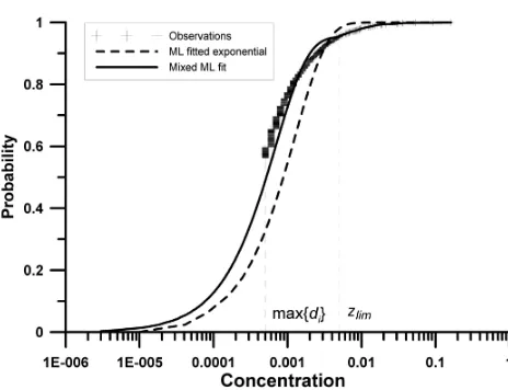
Fig. 1. The empiricel distribution of the observed arsenic concen-trations (crosses) for the values above the highest detection limit and the distributions obtained fitted via maximum likelihood for the whole dataset (dashed line) and with settingzlim to 0.005 mg l−1 (solid line).
4.2 Parameter estimation
As a first step the marginal distributions were estimated us-ing the approach described in Sect. 2.1. Figure 1 shows the distribution functions for arsenic. The estimation method was compared to the full maximum likelihood (Eq. 1 which would correspond to zlim>max(zi,i=1,...,Iin Eq. 2)). The empirical distribution function is only defined for val-ues above the highest detection limit.The traditional maxi-mum likelihood estimation is strongly influenced by outliers, leading to unrealistic, and unacceptable results. In contrast, settingzlimsuch thatzlim>max(dj,j=1,...,J )and bearing in mind that there are at least a few (30 or more in our case) exact measurement values (zis) belowzlim, leads to a good
[image:6.595.50.282.225.403.2]fit of the observed values, but one can see a slight break in the distribution function atzlim.
Fig. 2. The distribution of chloride concentrations and the estimated distributions corresponding to different degrees of censoring.
In order to investigate the quality of the extension of the distribution to censored values the observed chloride con-centration values were artificially censored. Detection limits were set to the 15, 25, 35, 45, 55, 65, 75 and 85 % quan-tiles of the distribution. Figure 2 shows distribution functions corresponding to different detection limits for chloride. Note that in order to see any differences the x-axis is shown on a logarithmic scale. All distribution functions are very similar, showing that the upper middle part of the distribution can be well used to extend it to low values.
[image:6.595.309.547.228.393.2]Table 2. Parameters of the fitted copulas.
Gauss copula V-transformed copula
B A B A m k
Arsenic 0.750 1325 0.810 49 000 1.78 0.376
deethylatrazine 0.030 669 0.579 35 000 0.29 2.469
Chloride 0.620 11 539 0.449 27 500 1.98 0.147
4.3 Interpolation
In order to illustrate the properties of the interpolation method illustrative examples are first considered. Assume that the value at the center of a square is to be estimated, with observations at the four corners. Four different configu-rations are considered:
1. Assume two corners on a diagonal have exact values equal to the 0.5 quantile of the distribution.
2. Assume two corners on a diagonal have exact values equal to the 0.5 quantile of the distribution and the two other corners have censored values with the same de-tection limit which is equal to the 0.5 quantile of the distribution.
3. All corners have exact values equal to the 0.5 quantile of the distribution.
4. Assume two corners on a diagonal have exact values equal to the 0.5 quantile of the distribution and the two other corners have censored values one with a detection limit equal to the 0.5 quantile the other equal to the 0.1 quantile of the distribution.
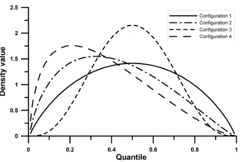
The spatial dependence structures of deethylatrazin were used for these examples. Figure 3 shows the conditional den-sities in the quantile space for the center of the square. Con-figuration one corresponds to the case if censored values are not considered corresponding togxe(z)in Eq. (22). This den-sity is modified in configuration 2 – the two values below the 0.5 quantile lead to a higher density for lower values. Config-uration 3 corresponds to the case when non-detects are set to the detection limit. This leads to an estimator with less un-certainty and with higher expectation than in configuration 2. Configuration 4 shows that a constraint corresponding to a low detection limit can substantially modify the density ob-tained by the interpolatioin.
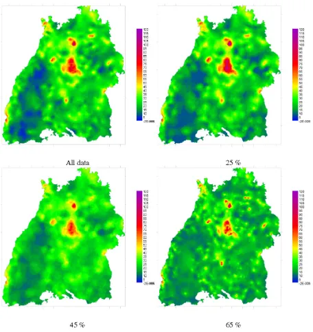
Figure 4 shows the interpolated maps for chloride using all observations and three different maps using 25 %, 45 % and 65 % censoring. Note the high similarity between the maps. The pointwise correlation between the map based on all observations and the maps obtained after censoring was calculated and is shown on Fig. 5. The correlation is constant
Fig. 3. Conditional densities obtained for the center of a square using different data at the corners.
– Configuration 1 two corners on a diagonal have exact values equal to the 0.5 quantile of the distribution.
– Configuration 2 two corners on a diagonal have exact values equal to the 0.5 quantile of the distribution and the two other corners have censored values with the same detection limit which is equal to the 0.5 quantile of the distribution.
– Configuration 3 all corners have exact values equal to the 0.5 quantile of the distribution.
– Configuration 4 two corners on a diagonal have exact values equal to the 0.5 quantile of the distribution and the two other corners have censored values one with a detection limit equal to the 0.5 quantile the other equal to the 0.1 quantile of the distribution
around 0.95 up to 65 %, and diminishes afterwards rapidly thereafter, reaching nearly 0 at 85 % censoring.
An advantage of the copula based approach is that it pro-vides the full conditional distribution for each location. Thus confidence intervals can be calculated, which are more real-istic than those obtained by kriging.
4.4 Comparison with other interpolation methods
Fig. 4. Interpolated chloride concentrations for different grades of censoring.
1. All values below the detection limit were set to zero. 2. All values below the detection limit were set to half of
the corresponding detection limit.
3. All values below the detection limit were set to the cor-responding detection limit.
Empirical variograms were calculated for each case. Ad-ditionally the empirical variogram was calculated from the exact values only. Figure 6 shows the graph of these vari-ograms for deethylatrazine. The exact values lead to a var-iogram without any structure and with the highest variance.
Fig. 5. Correlation between the interpolated map of Chloride and the maps interpolated from censored data.
Another popular method to treat highly skewed variables is indicator kriging (IK). The indicator corresponding to a cutoff valueαis defined as:
Iα(Z(x))=
0 ifZ(x) > α
1 ifZ(x)≤α (27)
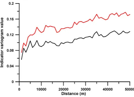
Indicator variograms are calculated for a set of α values. These do not suffer from the problem of outliers. A subse-quent IK leads for eachxandαto an estimated value which is usually interpreted as a probability of non-exceedance. The estimators corresponding to differentαvalues are then assembled to a distribution function. The expected value can then be calculated for each location. Censored data can be treated with indicators, namely forαvalues below the detec-tion limit the indicator remains undefined, while for above the indicator is 1. This is a correct treatment of the data, but leads to the problem that for each α below the lowest detection limit all indicator values equal zero. This means that the procedure is practically filling in the data with the detection limit, leading to similar biased estimators as OK. Figure 7 shows the graph of empirical indicator variograms for deethylatrazine. Note that in contrast to the empirical variograms of Fig. 6 these curves show a clear spatial depen-dence even without removing the outliers.
Lognormal kriging was not considered for this compar-ison, as it was reporeted the back transformation is very sensitive and might lead to problems with the estimator Roth (1998). Further the replacement of the non-detects would play a major role in the variogram estimation for this method.
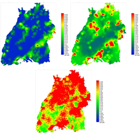
[image:9.595.48.287.73.227.2]Figure 8 shows the interpolated maps for deethylatrazine using the v-copula, IK and OK by setting all censored data equal to the corresponding detection limit. The OK maps show the typical problem the method has with skewed dis-tributions. The high values have a large influence, and lead to an overestimation. The map obtained by IK is more re-alistic. However the overestimation is still a problem here,
Fig. 6. Empirical variograms calculated for deethylatrasine, using exact data only (black solid), using nondetects replaced by zero (blue dashed) or by the detection limit (blue solid) and using non-detects replaced by zero and removal of outliers (red dashed).
Fig. 7. Empirical indicator variograms calculated for deethylatra-sine for the 85 % and 90 % values of the distribution.
as the values below the detection limit are practically set to the detection limit. The copula based interpolation allows in-terpolated values below the detection limit and, in doing so, leads to a plausible result.
[image:9.595.311.544.290.458.2]Fig. 8. Interpolated deethylatrazine concentrations using different interpolation methods. For OK the values were set to the detection limit.
Table 3. Cross validation results for Arsenic.
Measure V-copula Gauss-copula Indicator Ordinary Kriging
Kriging 50 % of Detection limit
MSQE 3.7×10⁻⁶ 1.0×10⁻⁵ 5.3×10⁻⁵ 1.0×10⁻⁵
Rank correlation 0.32 0.32 0.33 0.33
LEPS Score 0.142 0.154 0.142 0.159
[image:10.595.109.488.587.666.2]Table 4. Cross validation results for deethylatrazin.
Measure V-copula Gauss-copula Indicator Ordinary Kriging
Kriging 50 % of Detection limit
MSQE 5.1×10⁻⁴ 3.0×10⁻³ 5.0×10⁻³ 1.7×10⁻³
Rank correlation 0.44 0.31 0.40 0.48
LEPS Score 0.168 0.311 0.100 0.110
[image:11.595.50.283.198.365.2]Mean probability for<DTL 0.869 0.888 0.560 0.650
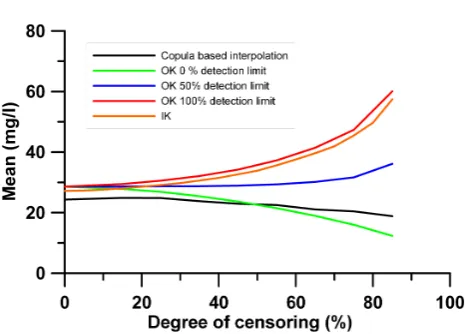
Fig. 9.Mean of the interpolated maps of Chloride for different degrees of censoring and different interpolations.
26
Fig. 9. Mean of the interpolated maps of Chloride for different degrees of censoring and different interpolations.
As a next step for all three variables and all interpola-tion methods a cross validainterpola-tion was carried out. The eval-uation of the cross validation results is not straightforward due to the censoring. The usual squared error is, even for the exact values, not appropriate as the distributions are highly skewed and some extreme outliers would dominate this mea-sure. Instead this measure was calculated by leaving out the upper 1 % of the measured values, ensuring that outliers were not considered for the calculation. Further the rank correlation for the exact values was calculated. Addition-ally the LEPS score (linear error in probability space) Ward and Folland (1991) was calculated to evaluate the fit in the probability space.
LEPS=1 n
n
X
i=1
|Gz(z(xi))−Gz(z∗(xi))| (28)
Herez∗(xi)is the expected value of the iterpolation
calcu-lated from the density obtained in Eq. (22).
For the measurements below the detection limit the aver-age of the probabilities to be below the detection limit was calculated.
Results for the two censored variables and for an artifi-cially censored case (chloride) are displayed in Tables 3 and 4. As one can see the copula based approaches outperform the ordinary and the indicator kriging. Note that the mean
Fig. 10.Frequency of observations in the 80 % confidence interval for V-copula based interpolation (long
dashes) and Gauss-copula based interpolation (short dashes) and indicator kriging (dashed dotted line) for
different grades of censoring of Chloride.
27
Fig. 10. Frequency of observations in the 80 % confidence interval for V-copula based interpolation (long dashes) and Gauss-copula based interpolation (short dashes) and indicator kriging (dashed dot-ted line) for different grades of censoring of Chloride.
squared error, the rank correlation and the LEPS score were all calculated for the exact measurements only. From the two copula models the v-copula allowing a non-symmetrical de-pendence is slightly better than the Gaussian.
[image:11.595.310.544.207.374.2]Table 5. Cross validation results for Chloride with 45 % artificial censoring.
Measure V-copula Gauss-copula Indicator Ordinary Kriging
Kriging 50 % of Detection limit
MSQE 273.1 251.8 298.6 2922.5
Rank correlation 0.61 0.61 0.58 0.45
LEPS Score 0.186 0.174 0.191 0.150
Mean probability for<DTL 0.593 0.555 0.000 0.390
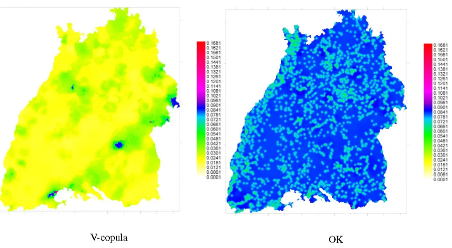
Fig. 11. Uncertainty maps for deethylatrazin: left the length of the 80 % confidence interval obtained via v-copula based interpolation, right the kriging standard deviation obtained by OK.
For interpolation and for possible random simulation of the fields a good measure of uncertainty is of great impor-tance. As the kriging variance is only a good measure of uncertainty when the data follow a multivariate normal dis-tribution. Else it is only a measure of data configuration, not data value dependent (especially for skewed distributions c.f. Journel, 1988) and it is not a good measure of uncertainty. The indicator approach provides estimates of the local con-ditional distribution functions. As it is not directly consid-ering the estimation uncertainty (all indicator values are in-terpolated values with no uncertainty associated) it does not provide a good uncertainty measure. The copula approach yields full probability distributions for each location, thus ar-bitrary confidence intervals can be derived. Figure 11 shows the width of the 80 % confidence interval obtained using v-copula based interpolation and the width of the 80 % confi-dence interval obtained using ordinary kriging under the
as-sumption of a normally distributed error for deethylatrazin. One can see that the estimation quality of the copula based interpolation is very heterogeneous over the whole domain. Regions with high observed values the confidence intervals are wide, in low areas narrow. For ordinary kriging the esti-mation error (kriging standard deviation) is small close to points with measured values, irrespective of the observed values.
[image:12.595.74.527.202.451.2]5 Conclusions
In this paper a methodology for the interpolation of variables with data below a detection limit was developed. As a first step the marginal distributions were estimated using a mixed approach which entailed a maximum likelihood method for the lower values and the empirical distribution for the high values. This procedure provides a robust estimator for the low concentrations without the negative influence of possi-ble outliers. Using the fitted distributions the variapossi-bles were transformed to the unit interval and their spatial copula was assessed, assuming spatial stationarity. Values below the de-tection limit are considered in a maximum likelihood estima-tion of the spatial copula parameters. Interpolaestima-tion was done by calculating the conditional distributions for each location. The conditions include both the measurements as exact val-ues and the below detection limit observations as inequality constraints.
The copula based interpolation is exact at the observation locations; the interpolated value equals the observed value. For locations with censored observations the method pro-vides an updated distribution function which differs from the constrained marginal. Other procedures such as indica-tor kriging with inequality constraints do not update distribu-tions at observation locadistribu-tions.
Investigations based on the artificially censored dataset show that the copula-based approaches remain unbiased even for large degrees of censoring. Among the kriging ap-proaches only ordinary kriging with setting the censored val-ues equal to the half of the corresponding detection limit did not show a systematic error for higher detection limits. This choice is clearly better than setting the values below the de-tection limit equal to the dede-tection limit, or setting them all equal to zero, which both lead to systematic errors. Indica-tor kriging also shows a systematic bias increasing with the detection limit.
The copula-based approaches outperform ordinary and in-dicator kriging in their interpolation accuracy. Inin-dicator krig-ing is only slightly worse than the copula based interpolation, while ordinary kriging with all different considerations of the values below detection limit are the poorest estimators.
The main advantage of the copula based approaches is in the estimation of the interpolation uncertainty. While ordi-nary kriging yields unrealistic estimation variances depend-ing only on the configuration of the measurement locations, the copula-based interpolation yields reasonable confidence intervals. The v-copula based approach yields more realistic confidence intervals than the Gaussian alternative.
The suggested approach can be extended to handle any kind of inequality constraints both for spatial structure as-sessment and for interpolation.
The model can serve as a basis for conditional spatial simulation. It would be possible to extend the model to a Bayesian approach where prior distributions are assigned to individual locations.
Acknowledgements. Research leading to this paper was supported by the German Science Foundation (DFG), project number Ba-1150/12-2.
Edited by: H. Cloke
References
B´ardossy, A.: Copula-based geostatistical models for ground-water quality parameters., Water Resour. Res., 42, W11416, doi:10.1029/2005WR004754, 2006.
B´ardossy, A. and Li, J.: Geostatistical interpolation using copulas., Water Resour. Res., 44, W07412, doi:10.1029/2007WR006115, 2008.
Cohen, C.: Simplified Estimators for the Normal Distribution When Samples Are Singly Censored or Truncated., Technometrics, 1, 217–237, 1959.
Cohen, C.: Progressively Censored Sampling in the Three Parame-ter Log-Normal Distribution., Technometrics, 18, 99–103, 1976. Genz, A. and Bretz, F.: Comparison of Methods for the Compu-tation of Multivariate t-Probabilities, J. Comp. Graph. Stat., 11, 950–971, 2002.
Helsel, D. R.: More than obvious: Better methods for interpret-ing nondetect data., Environmental Science and Technology, 39, 419A–423A, 2005.
Helsel, D. R. and Cohn, T. A.: Estimation of descriptive statistics for multiply censored water quality data., Water Resour. Res., 24, 1997–2004, 1988.
Journel, A. G.: New Distance Measures: The Route Toward Truly Non-Gaussian Geostatistics, Mathematical Geology, 20, 459– 475, 1988.
Keef, C., Tawn, J., and Svensson, C.: Spatial risk assessment for ex-treme river flows, Journal of the Royal Statistical Society Series C Applied Statistics, 58, 601–618, 2009.
Roth, C.: Is lognormal kriging suitable for local estimation?, Math-ematical Geology, 30, 999–1009, 1998.
Saito, H. and Goovaerts, P.: Geostatistical interpolation of posi-tively skewed and censored data in a dioxin-contaminated site., Environmental Science and Technology, 44, 4228–4235, 2000. Sedda, L., Atkinson, P. M., Barca, E., and Passarella, G.: Imputing
censored data with desirable spatial covariance function proper-ties using simulated annealing., J. Geogr. Syst., 36, 3345–3353, 2010.
Shumway, R., Azari, R., and Kayhanian, M.: Statistical Approaches to Estimating Mean Water Quality Concentrations with Detec-tion Limits., Environmental Science and Technology, 36, 3345– 3353, 2002.