https://doi.org/10.5194/hess-21-4825-2017 © Author(s) 2017. This work is distributed under the Creative Commons Attribution 3.0 License.
A hydrological prediction system based on the SVS land-surface
scheme: efficient calibration of GEM-Hydro for streamflow
simulation over the Lake Ontario basin
Étienne Gaborit1, Vincent Fortin1, Xiaoyong Xu2, Frank Seglenieks3, Bryan Tolson2, Lauren M. Fry4, Tim Hunter5, François Anctil6, and Andrew D. Gronewold5
1Environment Canada, Environmental Numerical Prediction Research (E-NPR), Dorval, H9P1J3, Canada 2University of Waterloo, Civil and Environmental Engineering Dpt., Waterloo, N2L3G1, Canada
3Environment Canada, Boundary Water Issues, Burlington, L7S1A1, Canada
4U.S. Army Corps of Engineers, Detroit District, Great Lakes Hydraulics and Hydrology Office, Detroit, MI 48226, USA 5NOAA Great Lakes Environmental Research Laboratory (GLERL), Ann Arbor, MI 48108, USA
6Civil and Water Engineering department, Université Laval, Québec, G1V0A6, Canada
Correspondence to:Étienne Gaborit ([email protected]) Received: 28 September 2016 – Discussion started: 1 November 2016
Revised: 24 July 2017 – Accepted: 8 August 2017 – Published: 28 September 2017
Abstract.This work explores the potential of the distributed GEM-Hydro runoff modeling platform, developed at Envi-ronment and Climate Change Canada (ECCC) over the last decade. More precisely, the aim is to develop a robust imple-mentation methodology to perform reliable streamflow sim-ulations with a distributed model over large and partly un-gauged basins, in an efficient manner. The latest version of GEM-Hydro combines the SVS (Soil, Vegetation and Snow) land-surface scheme and the WATROUTE routing scheme. SVS has never been evaluated from a hydrological point of view, which is done here for all major rivers flowing into Lake Ontario. Two established hydrological models are con-fronted to GEM-Hydro, namely MESH and WATFLOOD, which share the same routing scheme (WATROUTE) but rely on different land-surface schemes. All models are calibrated using the same meteorological forcings, objective function, calibration algorithm, and basin delineation. GEM-Hydro is shown to be competitive with MESH and WATFLOOD: the NSE √ (Nash–Sutcliffe criterion computed on the square root of the flows) is for example equal to 0.83 for MESH and GEM-Hydro in validation on the Moira River basin, and to 0.68 for WATFLOOD. A computationally efficient strategy is proposed to calibrate SVS: a simple unit hydro-graph is used for routing instead of WATROUTE. Global and local calibration strategies are compared in order to esti-mate runoff for ungauged portions of the Lake Ontario basin.
Overall, streamflow predictions obtained using a global cal-ibration strategy, in which a single parameter set is iden-tified for the whole basin of Lake Ontario, show accuracy comparable to the predictions based on local calibration: the average NSE √ in validation and over seven subbasins is 0.73 and 0.61, respectively for local and global calibrations. Hence, global calibration provides spatially consistent pa-rameter values, robust performance at gauged locations, and reduces the complexity and computation burden of the cali-bration procedure. This work contributes to the Great Lakes Runoff Inter-comparison Project for Lake Ontario (GRIP-O), which aims at improving Lake Ontario basin runoff simula-tions by comparing different models using the same input forcings. The main outcome of this study consists in a new generalizable methodology for implementing a distributed hydrologic model with a high computation cost in an effi-cient and reliable manner, over a large area with ungauged portions, using global calibration and a unit hydrograph to replace the routing component.
Creative Commons Attribution 3.0 License and the OGL are interoperable and do not conflict with, reduce or limit each other.
© Crown copyright 2017
1 Introduction
Given the continuous increase in precipitation forecast skill of numerical weather prediction (NWP) systems (Sukovich et al., 2014), it became possible to obtain skillful runoff forecasts directly from NWP model outputs, and streamflow forecasts by routing these gridded runoff fields. Indeed, mod-ern NWP models tend to simulate to some extent the snow, vegetation, and soil processes that contribute to the gener-ation of runoff and streamflow. In practice, however, many limitations are still associated with the representation of such processes in NWP systems, which were documented in Clark et al. (2015) and Davison et al. (2016).
Hydrological processes simulated by land-surface schemes (LSS) have been increasingly integrated into NWP models (Balsamo et al., 2009; Masson et al., 2013; Alavi et al., 2016; Wagner et al., 2016), as soil water content and snow water equivalent are recognized as key state variables for streamflow forecasting (Koster et al., 2004; Entekhabi et al., 2010). Environment and Climate Change Canada (ECCC), which provides operational weather and environmental forecasts within its boundary, is currently in the process of implementing a major upgrade to the LSS of the Global Environmental Multi-scale model (GEM), the national model. This new scheme, named SVS for soil, vegetation and snow, has been devised to assimilate space-based soil moisture retrievals as well as surface data, and has proven efficient at simulating soil moisture and brightness temperature (Alavi et al., 2016; Husain et al., 2016). SVS will be used to replace the Canadian version of the ISBA (Interaction Sol-Biosphère-Atmosphère) scheme that has been used in GEM since 2001 (Bélair et al., 2003). One of this paper’s objectives is to present the first evaluation of the capabilities of the new SVS scheme for streamflow prediction in Canada.
GEM’s LSSs can be run either two-way coupled to the mospheric model or offline, using GEM or other observed at-mospheric forcing. The platform for running GEM offline is known as GEM-Surf (Bernier et al., 2011). Runoff obtained from the LSS can then be routed to the outlet of the basin us-ing the WATROUTE routus-ing scheme (Kouwen, 2010). This configuration is known as GEM-Hydro.
Although the SVS scheme typically performed well for soil moisture simulations (e.g., Alavi et al., 2016; Husain et al., 2016), the capabilities of SVS to predict streamflow within the framework of GEM-Hydro, especially for large basins with ungauged portions, have not yet been examined. In this work, we present the calibration and evaluation of
GEM-Hydro based upon the SVS scheme for streamflow simulation over the Lake Ontario basin.
The Lake Ontario basin is chosen for the application of GEM-Hydro because the basin can favor the examination of GEM-Hydro (and SVS) performance for runoff simulation over a wide range of hydrological conditions (mixed vege-tation/land cover, natural/regulated regimes, gauged and un-gauged portions), and because there are a large amount of data available for model setup for this region.
be-cause of its typical use as a flood forecasting tool. Overall, it was difficult to attribute any difference in model results to the model structure, given that different forcing data and cal-ibration procedures had been used by each contributor to the project.
The GRIP project was extended next to Lake Ontario (GRIP-O) by Gaborit et al. (2017), who compared two lumped models, namely LBRM and GR4J (modèle du Génie Rural à 4 paramètres Journalier; Perrin et al., 2003), based upon the exact same forcing data and calibration framework. Two precipitation datasets were used as input: the Canadian Precipitation Analysis (CaPA; Lespinas et al., 2015), and a Thiessen polygon interpolation of the Global Historical Cli-matology Network – Daily (GHCND; Menne et al., 2012). CaPA is a near-real-time quantitative precipitation estimate product from ECCC that is available on a 10 km grid for all of North America (http://collaboration.cmc.ec.gc.ca/cmc/cmoi/ product_guide/submenus/capa_e.html).
The main finding of the first GRIP-O study is that the per-formance of the models was very satisfactory, resulting in an average NSE √(Nash–Sutcliffe criterion computed on the square root of the flows) in validation of 0.86 (over all subbasins and configurations), despite the fact that most trib-utaries have a regulated flow regime. This satisfactory per-formance justifies the use of CaPA as a precipitation forc-ing dataset in later studies, especially for distributed mod-els which require gridded precipitation as input. The perfor-mance of lumped models also provides a reference level of performance when evaluating distributed hydrological mod-els.
As an extension of the first GRIP-O study, the present work is focused on the evaluation of distributed hydro-logic models for Lake Ontario basin runoff simulations. Dis-tributed models typically have a broader range of applica-tions than lumped ones. For example, GEM-Hydro can be utilized to estimate the Lake Ontario net basin supplies (or NBSs, the sum of lake tributary runoff, overlake precipita-tion, and overlake evaporation: Brinkmann, 1983). However, distributed models are more complicated to calibrate and more computationally intensive, especially for large basins. The present study mainly aims at developing a methodology to improve the calibration efficiency of the distributed GEM-Hydro model for streamflow modeling over the Lake Ontario basin, including its ungauged parts. The proposed methodol-ogy is transferable and can be applied to other sophisticated distributed models and large basins with ungauged parts. In order to assess the impact of the SVS land-surface scheme on runoff simulations, the GEM-Hydro model is compared with two other distributed models, which rely on the same routing scheme (WATROUTE) as used in GEM-Hydro but different land-surface schemes. The intercomparison of the three mod-els could also provide insight into avenues to further improve GEM-Hydro and to capture structural uncertainty in runoff simulations using the multi-model approach.
2 Methodology 2.1 Models
Three different platforms are compared in this study: MESH, WATFLOOD and GEM-Hydro. MESH and GEM-Hydro have in common a distributed representation of most hydro-logical processes occurring in a basin and a structure orga-nized around two main components: a LSS for the represen-tation of surface processes (evapotranspiration, infiltration, snow processes, water circulation in the soils), and a river routing scheme for simulating water transport in the streams, which consists of WATROUTE for all models. WATROUTE is a 1-D hydrologic routing model relying mainly on flow directions and elevation data (Kouwen, 2010). It routes to the basin outlet the surface runoff and recharge produced by the surface schemes. In WATROUTE, runoff directly feeds the streams while recharge can be provided to an optional lower zone storage (LZS) compartment, representing super-ficial aquifers, which releases water to the streams. WAT-FLOOD and GEM-Hydro make use of the LZS, whereas recharge from MESH feeds directly into the stream. WAT-FLOOD is not considered to include a LSS because it is not solving the energy balance, only the water balance, but it is distributed.
The version of MESH used in this study relies on version 3.6 of the Canadian LAnd Surface Scheme (CLASS). Each grid cell is subdivided in a number of tiles, and each tile is classified as belonging to one of the five grouped response units (GRUs), based on its land-use–soil-type combination. In this paper, we follow the local calibration strategy advo-cated by Haghnegahdar et al. (2014) for MESH (see section on calibration strategy).
GEM-Hydro is very similar to MESH, but is tied to the LSSs available in GEM: ISBA and SVS. A previous study on the same basin demonstrated the clear superiority of SVS over ISBA, especially in regard to the baseflow component of the streamflow (see Gaborit et al., 2016). We thus only use SVS with GEM-Hydro in this paper.
WATFLOOD (Kouwen, 2010) is a distributed model of in-termediate complexity that only needs precipitation and tem-perature as forcing, as opposed to MESH and GEM-Hydro which need additional atmospheric variables (see Supple-ment). It relies on the GRUs concept and on many empirical equations. WATFLOOD has been employed by Pietroniro et al. (2007) over the Great Lakes basin.
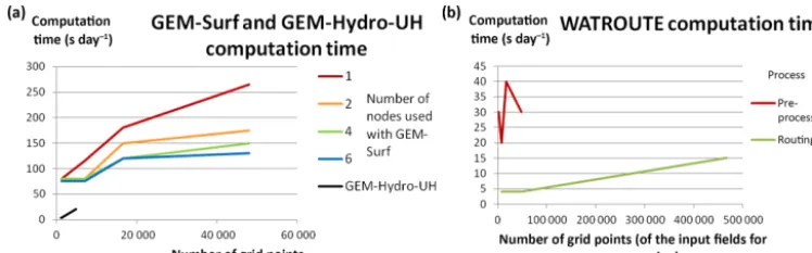
resolu-Figure 1.Computation time for GEM-Surf (land-surface part of GEM-Hydro), GEM-Hydro-UH and WATROUTE. See text for details. The number of grid points in this study is 1276 (476 000) for GEM-Surf/GEM-Hydro-UH (WATROUTE).
Table 1.Data sources. NAm: North America; n/a: not applicable.
Dataset/origin Type of data Coverage Resolution/scale Source
GSDE Soil texture Global ∼1 km (3000) Shangguan et al. (2014)
GLOBCOVER 2009 Land cover Global 300 m (1000) Bontemps et al. (2010) HydroSheds Flow directions Global ∼1 km (3000) Lehner et al. (2008)
SRTM DEM Global 90 m (300) USGS (2004)
HyDAT Gauge stations CAN NAm ECCC
NWIS Gauge stations US NAm USGS
CaPA v2.4b8 Precipitation n/a ∼15 km ECCC
RDPS Atmospheric forcings NAm 15/10 km ECCC
tion to save computation time for WATROUTE. The internal time step used for GEM-Hydro is 10 min. See Supplement for MESH and WATFLOOD implementation details. Table 1 shows the datasets used for physiographic information.
As the GEM-Hydro suite (including WATROUTE) is quite demanding in terms of computation time, it was decided to test a stand-alone configuration of GEM-Hydro relying on text files only and in which WATROUTE is replaced by a Unit Hydrograph (UH). This version is henceforth referred to as GEM-Hydro-UH. Figure 1 gives an overview of the relationship between computation time of the different mod-els and the dimension of their domain. Note that GEM-Surf (land-surface part of GEM-Hydro) was run on ECCC’s su-percomputer while GEM-Hydro-UH and WATROUTE were run on a machine with an AMD Athlon dual-core processor 4800+, because GEM-Hydro-UH and WATROUTE are not parallelized yet (their computation time would not change substantially if run on ECCC’s supercomputer).
The computation time for the experiment setup described here and when splitting the domain in four on an ECCC supercomputer is about 1.5 min day−1 for GEM-Surf, pro-vided that the pre-processing of the atmospheric variables was already done (which is the case in calibration: the pre-processing is done only once). WATROUTE (i.e., the routing part of GEM-Hydro) requires 25 s day−1 for the setup described here when running on a local machine. The WATROUTE pre-processing (i.e., preparation of the WA-TROUTE input files from the SVS outputs, which would
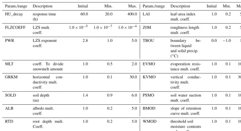
[image:4.612.103.492.250.360.2]perime-Table 2.Information on GEM-Hydro-UH 16 free parameters; LZS: lower zone storage; coeff.: coefficient; mult.: multiplicative; precip.: precipitation; param.: parameter; min.: minimum; max.: maximum.
Param./range Description Initial Min. Max. Param./range Description Initial Min. Max.
HU_decay response time (h)
60.0 20.0 400.0 LAI leaf-area index mult. coeff.
1.0 0.2 5.0
FLZCOEFF LZS mult. coeff.
1.0×10⁻⁵ 1.0×10⁻⁷ 1.0×10⁻⁴ Z0M roughness length mult. coeff.
1.0 0.2 5.0
PWR LZS exponent coeff.
2.8 1.0 5.0 TBOU boundary be-tween liquid and solid precip. (◦C)
0.0 −1.0 1.5
MLT coeff. To divide snowmelt amount
1.0 0.5 2.0 EVMO evaporation resis-tance mult. coeff.
1.0 0.1 10.0
GRKM horizontal con-ductivity mult. coeff.
1.0 0.1 30.0 KVMO vertical conduc-tivity mult. coeff.
1.0 0.1 30.0
SOLD soil depth (m)
1.4 0.9 6.0 PSMO soil water suction mult. coeff.
1.0 0.1 10.0
ALB albedo mult. coeff.
1.0 0.2 5.0 BMOD slope of retention curve mult. coeff.
1.0 0.1 10.0
RTD root depth mult. Coeff.
1.0 0.2 5.0 WMOD threshold soil moisture contents mult. coeff.
1.0 0.1 10.0
ter, and the maximum and minimum elevations along the basin main river. The UH lag time is also used as a free parameter during calibration (Table 2). This is inspired by the UH applied to the routing storage of GR4J (Perrin et al., 2003), but is employed here at an hourly time step. Finally, this framework allows a considerable reduction of compu-tation time and therefore allows us to perform calibration. However, GEM-Hydro-UH is faster than GEM-Hydro as long as the domain size remains of the order of a few thou-sand points (see Fig. 1). Beyond that threshold, not only is calibration no longer feasible with GEM-Hydro-UH, but it is possible that it becomes even slower than GEM-Hydro since the latter can be parallelized. Hydrographs resulting from GEM-Hydro and GEM-Hydro-UH can be very similar (Fig. 3). Finally, the SVS parameters identified by calibrating GEM-Hydro-UH are next transferred to the full version of GEM-Hydro, which then only needs WATROUTE Manning coefficients to be adjusted (if needed) in order to mimic the optimal hydrographs obtained with GEM-Hydro-UH. This last adjustment can be done manually with a few offline WA-TROUTE runs.
2.2 Study area and data
The GRIP-O spatial framework is defined in Fig. 2. A more detailed description of the area is available in Gaborit et al. (2017).
The Lake Ontario basin (Fig. 2) covers 83 000 km2, of which 19 000 km2is the lake surface. All upstream water
ar-Figure 2.GRIP-O spatial framework: Lake Ontario subbasin delin-eation (GRIP-O subbasins). GLAHF subbasins are from the Great Lakes Aquatic Habitat Framework (Wang et al., 2015). Dots (blue for natural flow regimes and red for regulated regimes) are the most-downstream flow gauges (i.e., the main tributaries’ gauges which are closest to Lake Ontario’s shoreline) selected for model calibra-tions.
[image:5.612.58.534.95.354.2] [image:5.612.308.549.389.552.2]On-tario, the lake outlet. Apart from some major cities (e.g., Toronto), the basin is mostly rural (agriculture, pasture, for-est), as shown in Danz et al. (2007).
Streamflow time series were selected based on their dura-tion and proximity to the lake shoreline. Of the 30 selected sites (Fig. 2), 27 have no missing data, 2 are complete at 94 %, and 1 at 80 % over the GRIP-O period. Nearly 70 % of the total Lake Ontario basin is gauged by the selected sites. Most of the rivers are regulated in some way, mainly for hy-dropower and flood mitigation, but regulation generally con-sists of reservoirs with a simple weir at their outlet (i.e., static control). Therefore, this did not prevent lumped models from registering good performance in the former GRIP-O study of Gaborit et al. (2017). As a consequence, no effort was made to represent in a detailed manner the artificial struc-tures of the region in WATROUTE. Moreover, the small di-versions occurring to fill some canals in the region, or even the aquifers which can contribute significantly to baseflow (Singer et al., 2003; Kassenaar and Wexler, 2006), do not prevent lumped models from registering good performance, which is helpful to this study.
The physiographic data required by the distributed mod-els under study consist of soil texture, land use/land cover, digital elevation model (DEM), and flow direction grids. Ta-ble 1 lists the datasets used to provide the physiographic and atmospheric inputs required by the models. There are 26 land cover classes are defined in GEM-Hydro. Soil tex-tures are from the Global Soil Dataset for Earth system mod-eling (GSDE; Shangguan et al., 2014), which contains in-formation down to 2.8 m. Soil texture was not calibrated for GEM-Hydro-UH, but some hydraulic parameters, which are derived from soil texture, were calibrated (Table 2). The max-imum soil depth is calibrated in GEM-Hydro-UH (Table 2) – see Supplement for MESH and WATFLOOD configuration details.
Precipitation forcings consist of 24-hourly accumulations from the Canadian Precipitation Analysis (CaPA version 2.4b8). Over the period of interest, CaPA consists of precipi-tation fields modeled by the Canadian Regional Determinis-tic Prediction System (RDPS,≈15 km resolution), corrected by local rain gauge observations (Lespinas et al., 2015). The daily CaPA accumulations were disaggregated on an hourly time step by following the temporal pattern of hourly pre-cipitation from the RDPS (Carrera et al., 2010). The remain-ing atmospheric forcremain-ings are taken from RDPS outputs, usremain-ing short-term forecasts having lead time of 6 to 18 h.
2.3 Calibration strategy
The GRIP-O experiment extends from 1 June 2004 to 26 September 2011. Calibrating a hydrologic model over a period of 4 to 5 years is generally deemed sufficient to achieve reasonable model robustness (e.g., Refsgaard and Knudsen, 1996). The calibration period thus ranges from 1 June 2007 to 26 September 2011 (4.5 years). Validation
is from 1 June 2005 to 1 June 2007 (2 years, the last one being used as spin-up for calibration), and spin-up from 1 June 2004 to 1 June 2005 (1 year). Note that during the automatic calibrations, the spin-up year was simulated only once and for all subsequent runs. The objective function is the Nash–Sutcliffe criterion (Nash and Sutcliffe, 1970) com-puted on the square root of the observed and simulated time series (Eq. 1), in order to avoid overemphasizing peak-flow events – henceforth referred to as “NSE√”:
NSE√=1− P
i=1,n
√
Qobsi−
√
Qsimi 2
P i=1,n
√ Qobsi−
√
Qobs
2. (1)
These decisions are consistent with the lumped modeling decisions made for GRIP-O in Gaborit et al. (2017). Other evaluation criteria used in this study consist in the common Nash–Sutcliffe criteria (NSE), the Nash criteria calculated over the log of the flows (“NSE Ln”), and a percent bias cri-teria (PBIAS, Eq. 2) assessing the simulation’s overall water budget fit: a positive value denotes a general tendency to un-derestimate flows, and vice versa:
PBIAS= P
i=1,n(Qobsi−Qsimi) P
i=1,n(Qobsi)
·100. (2)
All metrics are evaluated at the daily time step. Calibration relies for all models on the dynamically dimensioned search (DDS) algorithm (Tolson and Shoemaker, 2007). Calibra-tion cost did not allow models to be calibrated locally for all GRIP-O subbasins (Fig. 2), but only those shown in Fig. 5. One local calibration takes between 2 and 5 days of com-putation (400 model runs; see below). Table 2 lists the free parameters of GEM-Hydro. GEM-Hydro-UH was calibrated using multiplicative coefficients that adjust the spatially vary-ing values of a given parameter, leadvary-ing to a reasonable num-ber of free parameters (16) while preserving spatial variabil-ity – see Supplement for MESH and WATFLOOD calibration details.
It is important to emphasize that the approach used to cal-ibrate GEM-Hydro may result in unrealistic values for some parameters, as the multiplicative coefficients could bring them beyond the range of physical coherence. More pre-cisely, soil water content thresholds and albedo (Table 2) cannot be higher than 1. Therefore, these values were con-strained to realistic ranges after they were adjusted by the calibration algorithm by imposing them a minimum value of 0 and a maximum of 1.
Figure 3.Hydrographs from uncalibrated GEM-Hydro and GEM-Hydro-UH (Moira River – subbasin 11).
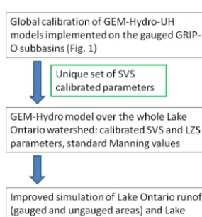
Figure 4.Diagram summarizing the methodology employed to sim-ulate Lake Ontario runoff with GEM-Hydro.
very efficient in the sense that it adjusts the search behavior to the maximum number of objective function evaluations (model runs) in order to converge to good quality solutions (Tolson and Shoemaker, 2007). The similarity of the perfor-mances obtained with GR4J and GEM-Hydro-UH (Fig. 5) supports the choice of the methodology used here, as GR4J was implemented with a maximum of 2000 model runs, three distinct calibration trials, and had an even lower number of free parameters (6; see Gaborit et al., 2017).
Even though the three models studied here were not cal-ibrated using the same number of free parameters and the same maximum allowed model runs (see Supplement), it is assumed that the calibration strategies employed allow each model to come very close to its optimal performance for a given subbasin and the time period considered. Indeed, the strategy used for each of the three models always involves parameters affecting the whole range of the main hydrolog-ical processes. The most important methodologhydrolog-ical consis-tencies for achieving a fair comparison between models in-clude, in our view, a common calibration algorithm and ob-jective function, along with common physiographic and forc-ing data.
Finally, some subbasins in Fig. 2 have more than one ma-jor tributary flowing into Lake Ontario. In this case, the most-downstream observed flows on independent tributaries are summed and then extrapolated to the whole subbasin using the area ratio method (ARM; Fry et al., 2014). The resulting “synthetic” flows were considered as observations for GEM-Hydro-UH calibration over the whole subbasin, including its ungauged parts. This methodology was applied to all sub-basins with more than one most-downstream gauge (identi-fied with the “n/a” mention for the station attribute in Ta-ble 3) for consistency with the calibration experiments per-formed in the first GRIP-O study (see Gaborit et al., 2017), and because lumped models (and GEM-Hydro-UH) can only estimate streamflow at one location. For these subbasins, the true gauged fraction is specified in Table 3.
2.4 Strategy for ungauged areas
The ultimate objective of the GRIP-O project consists in im-proving simulated Lake Ontario NBSs, which calls for es-timating runoff from all ungauged areas. To do so, calibra-tion was performed over the GRIP-O gauged area (which includes all GRIP-O gauged subbasins; see Fig. 2), and the resulting parameter set was used in the model imple-mented over the whole Lake Ontario basin, including its un-gauged parts. The “GRIP-O un-gauged area” is actually un-gauged at 88.5 % due to the strategy used for subbasins with several major tributaries (see end of previous section).
For GR4J, a single (unique) model was used over each of these two areas, requiring a unique calibration and a straight-forward parameter transfer. Hence, for GR4J, local calibra-tion was used but with a unique model for the GRIP-O gauged area.
GEM-Hydro-UH was, however, implemented locally for each of the gauged GRIP-O subbasins, but a global calibra-tion strategy (see further down) led to a unique calibrated parameter set which was then transferred to a GEM-Hydro model implemented over the whole Lake Ontario basin.
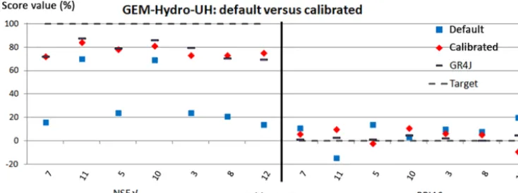
[image:7.612.95.238.242.395.2]Figure 5.Uncalibrated and calibrated GEM-Hydro-UH performances over the calibration period. Results are presented as NSE√(a)and PBIAS(b), for many GRIP-O subbasins. The gray dashed line shows perfect scores and GR4J reference is displayed with black markers.
Table 3.GRIP-O subbasin characteristics. n/a: not applicable.
Country Subbasin # Station %_gauged Area (km2) Flow regime Mean elev. (m)
CAN 1 20_mile n/a 307 natural 198
USA 3 Genessee n/a 6317 regulated 418
USA 4 bis Irondequoit n/a 326 natural 172
USA 5 Oswego n/a 13 287 regulated 259
USA 6 n/a 40 2406 mixed 264
USA 7 Black River n/a 4847 regulated 471
USA 8 Oswegatchie n/a 2543 regulated 250
CAN 10 Salmon_CA n/a 912 regulated 196
CAN 10 bis n/a 44.2 944 mixed 115
CAN 11 Moira n/a 2582 regulated 228
CAN 12 n/a 88 12 515.5 regulated 282
CAN 13 n/a 40.3 1537.5 natural 178
CAN 14 n/a 61.3 2689.4 mixed 209
CAN 15 n/a 63 2245.8 mixed 263
was preferred to other possible alternatives mainly because it allows taking into account rainfall over the ungauged areas as well as rainfall over the gauged areas, or, in other words, to use the best approximation of rainfall.
The global calibration of GEM-Hydro-UH consists in finding a unique trade-off parameter set that allows for si-multaneous improvement in performances for all subbasins (Ajami et al., 2004; Haghnegahdar et al., 2014; Gaborit et al., 2015), whereas local calibration consists in finding each subbasin’s optimal parameter set. Local calibration logically leads to the optimal performances for a given subbasin, but global calibration may lead to temporal robustness (Gaborit et al., 2015) and spatial consistency of the parameter values, because they are either fixed or adjusted the same way over the whole area under study. Local calibration, on the other hand, because of equifinality and experiment imperfections (model processes, forcing data, observed flows, etc.), may compensate for simulation errors and lead to parameter sets that do not work well when transferred to other (even neigh-bor) subbasins, as suggested by the fact that very different
parameter sets were obtained here with the local calibrations of GEM-Hydro-UH (Sect. 2.1 and Table 4). Global calibra-tion is not exempt from equifinality issues either, but to a lesser degree than local calibration. Indeed, the use of global parameters constrains parameter values across the basin to be equal and thus provides less freedom to achieve the same overall performance with different parameter sets. Moreover, the attention paid to the parameter ranges used (Table 2) al-lows us to be confident in the physical relevance of the final parameter values.
The objective function associated to global calibration of GEM-Hydro-UH is as follows:
OF=XN
i=1
1− Nloci Nglobi
, (3)
with Nloci the NSE
√
value calculated from the local cali-bration on subbasini, and Nglobithe NSE
√
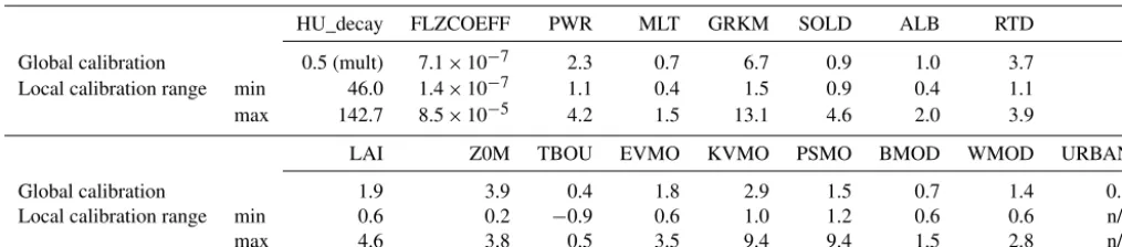
Table 4.Final parameter values or ranges after calibration; for global calibration, HU_decay consists of a multiplicative coefficient. See Table 2 for parameter definition. n/a: not applicable.
HU_decay FLZCOEFF PWR MLT GRKM SOLD ALB RTD
Global calibration 0.5 (mult) 7.1×10⁻⁷ 2.3 0.7 6.7 0.9 1.0 3.7
Local calibration range min 46.0 1.4×10⁻⁷ 1.1 0.4 1.5 0.9 0.4 1.1
max 142.7 8.5×10⁻⁵ 4.2 1.5 13.1 4.6 2.0 3.9
LAI Z0M TBOU EVMO KVMO PSMO BMOD WMOD URBAN
Global calibration 1.9 3.9 0.4 1.8 2.9 1.5 0.7 1.4 0.7
Local calibration range min 0.6 0.2 −0.9 0.6 1.0 1.2 0.6 0.6 n/a
max 4.6 3.8 0.5 3.5 9.4 9.4 1.5 2.8 n/a
GEM-Hydro-UH was not locally calibrated for all of the 14 GRIP-O subbasins (only those of Fig. 5 because of the com-putation cost), performances obtained with local GR4J cal-ibrations (Gaborit et al., 2017) were used for missing ones, justifying the use of that model in this study.
With global calibration, the response time parameter con-trolling the UH duration (Table 2) was replaced with a mul-tiplicative factor adjusting the default response times of all local subbasins.
Models were finally implemented over the whole Lake Ontario basin (Fig. 2), and runoff simulations performed with the parameter sets calibrated over the GRIP-O gauged area. Hydro was selected for this task instead of GEM-Hydro-UH since it was more straightforward and a priori more realistic (see further) to use WATROUTE instead of the simple UH for the ungauged areas of the Lake Ontario basin. In GEM-Hydro, standard Manning coefficients were used in WATROUTE, while the lag time of GEM-Hydro-UH was ad-justed during calibration. But it was assessed that simulations with GEM-Hydro (calibrated SVS and LZS parameters and standard Manning values) were very close, both in terms of hydrographs and performances at the gauged sites, to those from the calibrated GEM-Hydro-UH. Figure 4 summarizes the methodology described here for estimating runoff from the ungauged areas of the Lake Ontario basin with GEM-Hydro.
3 Results
The comparison between GEM-Hydro and GEM-Hydro-UH is first presented to demonstrate the relevance of the UH ap-proach to save the computation time associated with running the routing model of GEM-Hydro. Score improvements ob-tained by calibrating GEM-Hydro-UH for several subbasins of Lake Ontario basin are then presented, followed by a per-formance comparison for all models. Finally, the methodol-ogy proposed with GEM-Hydro and the lumped GR4J model to simulate streamflows for the ungauged parts of the Lake Ontario basin is evaluated.
Figure 3 presents the hydrographs simulated for the Moira River (subbasin 11 in Fig. 2), with SVS default parameters, standard WATROUTE parameter values in the case of GEM-Hydro, and a UH lag time estimated with the Epsey method in the case of GEM-Hydro-UH. As can be seen from this figure, GEM-Hydro-UH is able to produce streamflow sim-ulations which are very close to those obtained with GEM-Hydro, underlying the relevance of such an approach to save computation time. Between the uncalibrated GEM-Hydro and GEM-Hydro-UH performances and over the different GRIP-O subbasins, the average absolute difference in NSE√ was 8 %, with the worst difference being 21 % (GEM-Hydro being most of the time better than GEM-Hydro-UH). A com-plete GEM-Hydro run over the GRIP-O calibration period (4.5 years) takes about 48 h, while the GEM-Hydro-UH ver-sion requires only 1.2 h over the same period.
3.1 GEM-Hydro-UH local calibrations
This section presents GEM-Hydro-UH performances (Fig. 5) either with its default parameter values or after its local cali-bration on Lake Ontario subbasins, whose characteristics are given in Table 3.
As can be seen from Fig. 5, calibration provides substan-tial improvements in NSE√values. Similar results were ob-tained for NSE and NSE Ln (although these results are not shown), and a lower improvement for PBIAS; Interestingly, all uncalibrated NSE√ are above zero (Fig. 5), and even satisfactory for subbasins 10 and 11. This is encouraging for ungauged subbasin applications. It can also be noticed in Fig. 5 that calibration sometimes inverts the sign of the PBIAS criteria (switching from over- to under-estimation or vice versa).
ob-Table 5.Performance for the GRIP-O gauged area and the whole Lake Ontario basin (Fig. 2) with GR4J and globally calibrated GEM-Hydro-UH and GEM-Hydro models. Cal., val.: calibration and validation periods, respectively.
GRIPO gauged area: 53 459.2 km2 Lake Ontario basin: 68 214.8 km2
GR4J GEM-Hydro-UH GEM-Hydro GR4J GEM-Hydro
Scores (%) cal val cal val cal val cal val cal val
NSE 82.4 84.6 80.1 83.4 79.8 80.5 82.9 85.5 81.8 82.0
NSE√ 84.7 85.5 83.0 86.6 78.5 82.4 84.4 85.0 80.5 83.7
NSE Ln 83.3 84.0 82.1 87.2 74.4 82.3 82.4 82.8 76.8 83.7
PBIAS −0.3 1.5 −9.0 −8.1 −13.1 −10.9 −2.2 −1.2 −10.3 −8.2
servations come from the SNow Data Assimilation System (SNODAS; see NOHRSC, 2004). Calibration does influence evapotranspiration, but no observations are available to eval-uate this model output. For example, for the Moira River, the mean subbasin annual evapotranspiration (over the calibra-tion period) is equal to 527 mm and to 647 mm, before and after calibration respectively. The robustness of the model is also deemed very good, since performances do not sub-stantially deteriorate between calibration and validation (Ta-ble 5).
Calibrated parameter values are quite different from one subbasin to the other (even for neighbor subbasins), which may be due to equifinality (different parameter sets can lead to similar simulations) but also to the anthropogenic stream-flow regulations. Table 4 presents the ranges of the final pa-rameter values obtained with local calibration. This strongly limits the potential for parameter transferability to ungauged subbasins (Razavi and Coulibaly, 2012; Parajka et al., 2013). As explained in Sect. 1.4, global calibration can help over-come this by leading to a spatially coherent parameter set. Results of such an approach are presented in Sect. 2.3.
Calibrated GEM-Hydro-UH performance values are gen-erally very close to those obtained with GR4J and CaPA pre-cipitation (Fig. 5): the mean absolute difference in NSE√ values is 6.1 %, with the maximum being 15 % (GR4J be-ing generally better). This is very encouragbe-ing as the perfor-mance benchmark set by GR4J simulations is most of the time quite high and hard to attain for other models.
3.2 Inter-comparison of all models
This section aims at comparing MESH, WATFLOOD and GEM-Hydro-UH, but detailed results specific to MESH and WATFLOOD are only provided in the Supplement to this pa-per. When looking closely at the Moira River hydrographs, for the three calibrated models (Fig. 6), important differences arise. For instance, WATFLOOD has a more flashy behavior and tends to overestimate peak flow events, MESH generally underestimates flows, and GEM-Hydro-UH lies somewhere in between. Peak flow events (even for other subbasins) as-sociated to the spring freshet are generally better represented by MESH, which may be due to a better representation by
CLASS of various cold regions hydrological processes, such as snow accumulation and melt, snow interception by vege-tation, as well as soil freezing and thawing. NSE√in vali-dation for this basin are respectively equal to 0.83, 0.68 and 0.83 for MESH, WATFLOOD and GEM-Hydro-UH. 3.3 Runoff estimation for the whole Lake Ontario
basin
The parameter values identified from the global calibration are presented in Table 4, along with the ranges resulting from local calibrations. See Sect. 1.4 for more information about methodology related to global calibration. It can be seen from Table 4 that final global parameters generally lay inside the intervals obtained from local calibration, highlighting the trade-off found by global calibration. Moreover, it was no-ticed (not shown here) that parameter values were very dif-ferent between local and global calibration procedures, even for basins displaying very similar performances between the two strategies (such as subbasins 3, 5 and 8; see Fig. 7), high-lighting the fact that local calibration is more prone to over-calibration (i.e., equifinality).
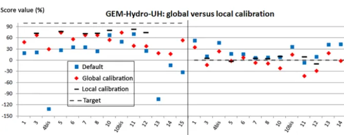
GEM-Hydro-UH results are given first for each gauged subbasin, in order to compare global calibration, local cal-ibration and default parameters (Fig. 7), followed by GR4J and GEM-Hydro results (with global calibration) for the GRIP-O gauged area and the whole Lake Ontario basin (Ta-ble 5 and Figs. 8–9).
[image:10.612.103.494.96.198.2]cal-Figure 6.Intercomparison for the Moira River (calibration period, CaPA precipitation).
Figure 7. GEM-Hydro-UH performances in validation for the 14 GRIP-O gauged subbasins (Fig. 2) with default, locally and globally calibrated parameter values. Perfect scores are shown. Results are presented as NSE√(a)and PBIAS(b).
ibration (Razavi and Coulibaly, 2012; Parajka et al., 2013). In this study, the strategy related to parameter transfer to the ungauged subbasins is based on spatial proximity, which was already identified as among the best parameter trans-fer methods for this type of climate in Canada (Razavi and Coulibaly, 2012). Although a comprehensive assessment of the reliability of the methodology used here for parameter transfer would require the “leave-one-out” framework (see Razavi and Coulibaly, 2012), the satisfying performances and temporal robustness obtained for all GRIP-O subbasins with global calibration, along with the spatial consistency of the unique final parameter set, the homogeneity of the area under study and the spatial proximity of ungauged basins together justify the relevance and a priori reliability of the methodology employed in this study. This statement is more-over supported by the evaluation performed for the whole basin in what follows.
Performance evaluation for the total GRIP-O gauged area (Table 5) shows that GR4J is better than GEM-Hydro-UH in calibration, but worse in validation. GEM-Hydro-UH leads to a very satisfactory performance, but most importantly to a better streamflow simulation than GR4J in terms of dy-namics (see Fig. 8). Note that the smoother GR4J behavior is not due to the single model approach for the whole area, as a similar behavior occurred when aggregating simulations from local GR4J models (Gaborit et al., 2017). This smooth
behavior seems inherent to the lumped attribute and concepts of GR4J. As depicted in Table 5, performances for the GRIP-O gauged area obtained with GEM-Hydro are close to those obtained with GEM-Hydro-UH, despite being lower for the former, which comes from the standard (uncalibrated) Man-ning coefficients used with GEM-Hydro, whereas the UH lag time was adjusted during the calibration of GEM-Hydro-UH. WATROUTE coefficients could have been manually tuned in order for GEM-Hydro performance values to reach those of GEM-Hydro-UH in Table 5, but this was not deemed nec-essary given the already very satisfying performance values obtained with the uncalibrated Manning values.
Runoff simulations for the whole Lake Ontario basin, in-cluding its ungauged areas, are very promising (Table 5). Even if runoff observations actually consist in this case in estimations based on the ARM, computed performances are a priori reliable given that the true gauged fraction of the total area is equal to about 70 %, and that the ARM proves reliable starting from a 50 % gauged fraction (Fry et al., 2014).
[image:11.612.131.466.224.355.2]Figure 8.Lake Ontario basin runoff (including its ungauged areas, Fig. 2) for the validation period, comparing GR4J and GEM-Hydro.
Figure 9.Cumulative Lake Ontario NBS (net basin supply) estimates. Months are shown on thexaxis. See text for further details.
Finally, Lake Ontario monthly NBSs were estimated with the globally calibrated GEM-Hydro model, and results were compared both to the GLERL residual and component NBS estimates (Fig. 9). Residual NBSs rely on the lake observed change in storage and streamflows for the Niagara and St. Lawrence rivers (DeMarchi et al., 2009). Component NBSs used here are based on the GLERL Monthly Hydrome-teorological Database (GLM-HMD; Hunter et al., 2015), which relies on observed data extrapolated with the ARM for runoff, on observed data interpolated with the Thiessen poly-gon method for overlake precipitation, and on the Large Lake Thermodynamics lumped Model (LLTM) for overlake evap-oration. Component NBS estimates are updated on a regular basis. Data used in this work were updated on 2 August 2016. It is still unknown which of these two NBS estimation meth-ods (i.e., residual or component method) is the most accurate (DeMarchi et al., 2009).
It can be seen that the cumulated NBS estimates derived from the calibrated GEM-Hydro model (using global cali-bration) stand between the component and residual NBS esti-mates, but are closer to the latter ones. It is, however, difficult to draw any conclusion regarding the bias of these estima-tion methods given the uncertainty associated with NBS es-timates (DeMarchi et al., 2009). When comparing the GLM-HMD component NBS method to the calibrated GEM-Hydro simulation on a component-by-component basis, the main
difference between the two occurs for overlake evaporation, with evaporation from the component method being signifi-cantly lower than GEM-Hydro evaporation (not shown). This mainly explains why the NBS estimates from the compo-nent method are higher than the other estimates in Fig. 9. But again, it is not possible to accurately evaluate overlake evaporation estimates given the lack of observations for this variable. The uncalibrated GEM-Hydro model results in cu-mulative NBS estimations which are below all other NBS estimations, which tends to suggest that they are underes-timated. Therefore, the methodology proposed to calibrate GEM-Hydro seems to improve Lake Ontario NBS simula-tions.
4 Discussion and conclusion
[image:12.612.126.469.234.363.2]areas with a high urban cover fraction. This result is encour-aging because SVS is expected to replace ISBA in ECCC operational models in the coming years.
The model intercomparison study also indicates that there is still room to further improve SVS. For example, adding the soil freeze–thaw processes to the current SVS may im-prove GEM-Hydro simulations of runoff peaks in spring. Ad-ditionally, a new snow module (ISBA-ES) is also being im-plemented in SVS, which currently relies on a simple force– restore approach. Finally, work is under way to represent a surface of ponded water in each SVS grid cell, in order to represent subgrid-scale lakes and wetlands and to better ac-count for the delay associated with surface runoff transfer into the streams.
The calibrated GEM-Hydro-UH performance values are close to GR4J ones (Gaborit et al., 2017). The potential ben-efits of global calibration have been demonstrated here, as for a previous Hydrotel application (Gaborit et al., 2015). It achieves satisfactory performances for a large area with a unique calibration and favors temporal robustness, spatial consistency and parameter transferability. Therefore, one of this study’s main outcomes is the confirmation that global calibration is a very promising and efficient methodology to implement hydrologic models over large areas. It saves com-putation time and leads to a spatio-temporally robust param-eter set that can be transferred to nearby (ungauged) areas. This outcome is important because parameter transfer meth-ods derived from local calibration are still largely prone to failure. More studies still have to be performed with global calibration on other basins and with other hydrological mod-els to confirm the value of this methodology, which worked well for the model and basin studied here. Global calibra-tion of SVS is envisioned in future versions of the WCPS, to assess its benefits in improving weather forecasts, as a calibrated SVS could be coupled to the RDPS atmospheric model, and because a calibrated SVS version should im-prove surface flux representation. Calibrating a LSS based on streamflow and then using it in an atmospheric model to improve weather forecasts has not been reported in the lit-erature so far, to our best knowledge. Another originality of this work which may be of interest to a broad audience is the way the distributed parameters were adjusted during cal-ibration. Instead of regrouping the parameters by GRU as for SA-MESH (see Supplement), which led to 60 free pa-rameters during calibration, GEM-Hydro-UH was calibrated with only 16 parameters, which consist mainly of multiplica-tive factors by which the associated actual parameter values were all multiplied the same way. This allows preserving the spatial variability and coherence of a given parameter, while minimizing the number of free parameters that still af-fect the whole domain. Of course, additive or exponent fac-tors could be used too, if deemed more relevant. This strat-egy is moreover suited to using the DSS algorithm, which allows a very fast convergence (in less than 400 iterations) when a limited number of free parameters are used, and
therefore contributes to the efficiency of the implementation methodology proposed here. Again, this could be applied to any distributed hydrologic model. Furthermore, in order to calibrate the GEM-Hydro model, its standard routing part was replaced by a simple UH during calibration of the land-surface scheme, the simpler setup requiring only 3 % of the original computation time. The routing component of GEM-Hydro can be run afterwards, and re-calibrated separately. Once again, the UH can be used with any LSS and on any basin, which allows us to calibrate a distributed model when the routing part is time-consuming, as for WATROUTE.
We developed a methodology (global calibration, multi-plicative factors used in calibration, and the UH bypass of the routing component) to improve the calibration efficiency and performance of the distributed GEM-Hydro model for streamflow modeling over the Lake Ontario basin, including its ungauged parts. The proposed methodology is transfer-able and can be useful to the hydrologic community, espe-cially for those who want to use distributed hydrologic mod-els to simulate streamflow for large basins with ungauged parts.
Finally, this work presented the development of an ef-ficient distributed hydrological modeling platform for the Lake Ontario basin, which can be used as a readily testing ground for distributed models. During the preparation and writing of this paper, using the proposed methodology in this study, GEM-Hydro was also applied to the Canadian Nel-son, Churchill and MacKenzie River basins as well as the whole Hudson Bay basin, with satisfactory performance val-ues. This is encouraging given the high degree of regulation involved in some of these basins.
Data availability. Data are available upon request from the first au-thor ([email protected]). For soil texture data, see Shang-guan et al. (2014). For Land Cover data, see Bontemps et al. (2010). For Flow direction data, see Lehner et al. (2008). For DEM data, see USGS (2004).
The Supplement related to this article is available online at https://doi.org/10.5194/hess-21-4825-2017-supplement.
Competing interests. The authors declare that they have no conflict of interest.
Edited by: Wouter Buytaert
Reviewed by: two anonymous referees
References
Ajami, N. K., Gupta, H., Wagener, T., and Sorooshian, S.: Calibra-tion of a semi-distributed hydrologic model for streamflow esti-mation along a river system, J. Hydrol., 298, 112–135, 2004. Alavi, N., Bélair, S., Fortin, V., Zhang, S., Husain, S. Z.,
Car-rera, M. L., and Abrahamowicz, M.: Warm Season Eval-uation of Soil Moisture Prediction in the Soil, Vegetation and Snow (SVS) Scheme, J. Hydrometeorol., 17, 2315–2332, https://doi.org/10.1175/JHM-D-15-0189.1, 2016.
Almeida, I. K., Almeida, A. K., Anache, J. A. A., Steffen, J. L., and Alves Sobrinho, T.: Estimation on time of concentration of overland flow in watersheds: a review, Geociências, 33, 661–671, 2014.
Balsamo, G., Beljaars, A., Scipal, K., Viterbo, P., van den Hurk, B., Hirschi, M., and Betts, A. K.: A revised hydrology for the ECMWF model: Verification from field site to terrestrial water storage and impact in the Integrated Forecast System, J. Hydrom-eteorol., 10, 623–643, https://doi.org/10.1175/2008JHM1068.1, 2009.
Bélair, S., Crevier, L. P., Mailhot, J., Bilodeau, B., and Delage, Y.: Operational implementation of the ISBA land surface scheme in the Canadian regional weather forecast model. Part I: Warm season results, J. Hy-drometeorol., 4, 352–370, https://doi.org/10.1175/1525-7541(2003)4<352:OIOTIL>2.0.CO;2, 2003.
Bernier, N. B., Bélair, S., Bilodeau, B., and Tong, L.: Near-surface and land surface forecast system of the Vancouver 2010 Winter Olympic and Paralympic Games, J. Hydrometeorol., 12, 508– 530, https://doi.org/10.1175/2011JHM1250.1, 2011.
Bontemps, S., Defourny , P., and Eric., V. B.: GlobCOVER 2009 products description and validation report, UCLouvain and ESA, available at: http://xa.yimg.com/kq/groups/17314041/ 1329044743/name/GLOBCOVER2009_Validation_Report_1.0. pdf (last access: 21 September 2017), 2010.
Brinkmann, W. A. R.: Association between net basin supplies to Lake Superior and supplies to the lower Great Lakes, J. Great Lakes Res., 9, 32–39, 1983.
Burnash, R. J. C.: The NWS river forecast system – catchment mod-elling, in: Computer Models of Watershed Hydrology, edited by: Singh, V., Water Resources Publications, Highlands Ranch, CO, 311–366, 1995.
Carrera, M. L., Bélair, S., Fortin, V., Bilodeau, B., Charpentier, D., and Doré, I.: Evaluation of snowpack simulations over the Cana-dian Rockies with an experimental hydrometeorological model-ing system, J. Hydrometeorol., 11, 1123–1140, 2010.
Clark, M. P., Fan, Y., Lawrence, D. M., Adam, J. C., Bolster, D., Gochis, D. J., Hooper, R. P., Kumar, M., Leung, L. R., Mackay, D. S., and Maxwell, R. M.: Improving the representation of hy-drologic processes in Earth System Models, Water Resour. Res., 51, 5929–5956, 2015.
Coon, W. F., Murphy, E. A., Soong, D. T., and Sharpe, J. B.: Com-pilation of watershed models for tributaries to the Great Lakes, United States, as of 2010, and identification of watersheds for
future modeling for the Great Lakes Restoration Initiative, US Geological Survey, Troy, NY, Open File Rep., 2011–1202, 2011. Croley, T. E. and He, C.: Great Lakes large basin runoff modeling, in: Proceedings of the Second Federal Interagency Hydrologic Conference, Las Vegas, NV, July 2002.
Danz, N. P., Niemi, G. J., Regal, R. R., Hollenhorst, T., Johnson, L. B., Hanowski, J. M., Axler, R. P., Ciborowski, J. J., Hrabik, T., Brady, V. J., and Kelly, J. R.: Integrated measures of anthro-pogenic stress in the US Great Lakes basin, Environ. Manage., 39, 631–647, 2007.
Davison, B., Pietroniro, A., Fortin, V., Leconte, R., Mamo, M., and Yau, M. K.: What is Missing from the Prescription of Hydrology for Land Surface Schemes?, J. Hydrometeorol., 17, 2013–2039, https://doi.org/10.1175/JHM-D-15-0172.1, 2016.
Deacu, D., Fortin, V., Klyszejko, E., Spence, C., and Blanken, P. D.: Predicting the net basin supply to the Great Lakes with a hydrometeorological model, J. Hydrometeorol., 13, 1739–1759, 2012.
DeMarchi, C., Dai, Q., Mello, M. E., and Hunter, T. S.: Estimation of Overlake Precipitation and Basin Runoff Uncertainty, Interna-tional Upper Great lakes Study, Case Western Reserve Univer-sity, Cleveland, OH, 64 pp., 2009.
Durnford, D., Fortin, V., Smith, G., Archambault, B., Deacu, D., Dupont, F., Dyck, S., Martinez, Y., Klyszejko, E., MacKay, M., Liu, L., Pellerin, P., Pietroniro, A., Roy, F., Vu, V., Winter, B., Yu, W., Spence, C., Bruxer, J., and Dickhout, J.: Towards an op-erational water cycle prediction system for the Great Lakes and St. Lawrence River, B. Am. Meteorol. Soc., in press, 2017. Entekhabi, D., Njoku, E. G., O’Neill, P. E., Kellogg, K. H.,
Crow, W. T., Edelstein, W. N., Entin, J. K., Goodman, S. D., Jackson, T. J., Johnson, J., and Kimball, J.: The soil mois-ture active passive (SMAP) mission, P. IEEE, 98, 704–716, https://doi.org/10.1126/science.1100217, 2010.
Fry, L. M., Gronewold, A. D., Fortin, V., Buan, S., Clites, A. H., Luukkonen, C., Holtschlag, D., Diamond, L., Hunter, T., Segle-nieks, F., Durnford, D., Dimitrijevic, M., Subich, C., Klyszejko, E., Kea, K., and Restrepo, P.: The Great Lakes Runoff Intercom-parison Project Phase 1: Lake Michigan (GRIP-M). J. Hydrol., 519, 3448–3465, https://doi.org/10.1016/j.jhydrol.2014.07.021, 2014.
Gaborit, É., Ricard, S., Lachance-Cloutier, S., Anctil, F., and Tur-cotte, R.: Comparing global and local calibration schemes from a differential split-sample test perspective, Can. J. Earth Sci., 52, 990–999, https://doi.org/10.1139/cjes-2015-0015, 2015. Gaborit, É., Fortin, V., and Tolson, B.: Great Lakes Runoff
In-tercomparison Project for Lake Ontario (GRIP-O), Environ-ment and Climate Change Canada, Dorval, QC, internal re-port, available at: http://collaboration.cmc.ec.gc.ca/science/rpn/ publications/pdf/GRIPO_report.pdf (last access: 18 September 2017), 133 pp., 2016.
Gaborit, É., Fortin, V., Tolson, B., Fry, L., Hunter, T., and Gronewold, D.: Great Lakes Runoff Inter-comparison Project, Phase 2: lake Ontario (GRIP-O), J. Great Lakes Res., 43, 217– 227, https://doi.org/10.1016/j.jglr.2016.10.004, 2017.
Gronewold, A. D., Clites, A. H., Hunter, T. S., and Stow, C. A.: An appraisal of the Great Lakes advanced hydrologic prediction system, J. Great Lakes Res., 37, 577–583, 2011.
Hunter, T. S., Clites, A. H., Campbell, K. B., and Gronewold, A. D.: Development and application of a North American Great Lakes hydrometeorological database – Part I: Precipitation, evapora-tion, runoff, and air temperature, J. Great Lakes Res., 41, 65–77, https://doi.org/10.1016/j.jglr.2014.12.006, 2015.
Husain, S. Z., Alavi, N., Bélair, S., Carrera, M., Zhang, S., Fortin, V., Abrahamowicz, M., and Gauthier, N.: The Multi-Budget Soil, Vegetation, and Snow (SVS) Scheme for Land Surface Param-eterization: Offline Warm Season Evaluation, J. Hydrometeo-rol., 17, 2293–2313, https://doi.org/10.1175/JHM-D-15-0228.1, 2016.
Kassenaar, J. D. C. and Wexler, E. J.: Groundwater Modelling of the Oak Ridges Moraine Area, York, Peel, Durham, Toronto and The Conservation Authorities Moraine Coalition (YPDT-CAMC), ON, CAMC-YPDT Technical Report #01–06, 2006. Koster, R. D., Dirmeyer, P. A., Guo, Z., Bonan, G., Chan,
E., Cox, P., Gordon, C. T., Kanae, S., Kowalczyk, E., Lawrence, D., and Liu, P.: Regions of strong coupling be-tween soil moisture and precipitation, Science, 305, 1138–1140, https://doi.org/10.1126/science.1100217, 2004.
Kouwen, N.: WATFLOOD/WATROUTE Hydrological model rout-ing & flow forecastrout-ing system, Department of Civil Engineerrout-ing, University of Waterloo, Waterloo, ON, 267 pp., 2010.
Lehner, B., Verdin, K., and Jarvis, A.: New global hydrography de-rived from spaceborne elevation data, EOS T. Am. Geophys. Un., 89, 93–94, https://doi.org/10.1029/2008EO100001, 2008. Lespinas, F., Fortin, V., Roy, G., Rasmussen, P., and Stadnyk, T.:
Performance Evaluation of the Canadian Precipitation Analysis (CaPA), J. Hydrometeorol., 16, 2045–2064, 2015.
Masson, V., Le Moigne, P., Martin, E., Faroux, S., Alias, A., Alkama, R., Belamari, S., Barbu, A., Boone, A., Bouyssel, F., Brousseau, P., Brun, E., Calvet, J.-C., Carrer, D., Decharme, B., Delire, C., Donier, S., Essaouini, K., Gibelin, A.-L., Giordani, H., Habets, F., Jidane, M., Kerdraon, G., Kourzeneva, E., Lafaysse, M., Lafont, S., Lebeaupin Brossier, C., Lemonsu, A., Mahfouf, J.-F., Marguinaud, P., Mokhtari, M., Morin, S., Pigeon, G., Sal-gado, R., Seity, Y., Taillefer, F., Tanguy, G., Tulet, P., Vincendon, B., Vionnet, V., and Voldoire, A.: The SURFEXv7.2 land and ocean surface platform for coupled or offline simulation of earth surface variables and fluxes, Geosci. Model Dev., 6, 929–960, https://doi.org/10.5194/gmd-6-929-2013, 2013.
Menne, M. J., Durre, I., Vose, R. S., Gleason, B. E., and Houston, T. G.: An overview of the Global Historical Climatology Network-Daily Database, J. Atmos. Ocean. Tech., 29, 897–910, 2012. Nash, J. E. and Sutcliffe, J. V.: River flow forecasting through
con-ceptual models part I – a discussion of principles, J. Hydrol., 10, 282–290, 1970.
National Operational Hydrologic Remote Sensing Center (NOHRSC): Snow Data Assimilation System (SNODAS) Data Products at NSIDC, 2009–2011, National Snow and Ice Data Center, Boulder, Colorado, USA, 2004.
Parajka, J., Viglione, A., Rogger, M., Salinas, J. L., Sivapalan, M., and Bloeschl, G.: Hydrograph prediction in ungauged basins – a comparative assessment of studies, Geophysical Research Ab-stracts, 15, EGU2013-13126, 2013.
Perrin, C., Michel, C., and Andréassian, V.: Improvement of a parsi-monious model for streamflow simulation, J. Hydrol., 279, 275– 289, 2003.
Pietroniro, A., Fortin, V., Kouwen, N., Neal, C., Turcotte, R., Davi-son, B., Verseghy, D., Soulis, E. D., Caldwell, R., Evora, N., and Pellerin, P.: Development of the MESH modelling system for hy-drological ensemble forecasting of the Laurentian Great Lakes at the regional scale, Hydrol. Earth Syst. Sci., 11, 1279–1294, https://doi.org/10.5194/hess-11-1279-2007, 2007.
Razavi, T. and Coulibaly, P.: Streamflow prediction in ungauged basins: review of regionalization methods, J. Hydrol. Eng., 18, 958–975, 2012.
Refsgaard, J. C. and Knudsen, J.: Operational validation and inter-comparison of different types of hydrological models, Water Re-sour. Res., 32, 2189–2202, 1996.
Shangguan, W., Dai, Y., Duan, Q., Liu, B., and Yuan, H.: A global soil dataset for earth system modeling, J. Adv. Model. Earth Syst., 6, 249–263, https://doi.org/10.1002/2013MS000293, 2014.
Sherman, L. K.: Streamflow from rainfall by the unit-graph method, Eng. News Record, 108, 501–505, 1932.
Singer, S. N., Cheng, C. K., and Scafe, M. G. (Eds.): The Hydroge-ology of southern Ontario, second ed., Environmental monitor-ing and reportmonitor-ing branch, Ministry of the Environment, Toronto, ON, 240 pp.+appendices, 2003.
Sukovich, E. M., Ralph, F. M., Barthold, F. E., Reynolds, D. W., and Novak, D. R.: Extreme quantitative precipitation forecast per-formance at the Weather Prediction Center from 2001 to 2011, Weather Forecast., 29, 894–911, https://doi.org/10.1175/WAF-D-13-00061.1, 2014.
Tolson, B. A. and Shoemaker, C. A.: Dynamically dimen-sioned search algorithm for computationally efficient water-shed model calibration, Water Resour. Res., 43, W01413, https://doi.org/10.1029/2005WR004723, 2007.
USGS: Shuttle Radar Topography Mission, 1 Arc Second scene SRTM_u03_n008e004, available at: https://www2.jpl.nasa.gov/ srtm/cbanddataproducts.html (last access: 21 September 2017), 2004.
Wagner, S., Fersch, B., Yuan, F., Yu, Z., and Kunstmann, H.: Fully coupled atmospheric-hydrological modelling at re-gional and long-term scales: Development, application, and analysis of WRF-HMS, Water Resour. Res., 52, 3187–3211, https://doi.org/10.1002/2015WR018185, 2016.
Wang, L., Riseng, C. M., Mason, L. A., Wehrly, K. E., Ruther-ford, E. S., McKenna, J. E., Castiglione, C., Johnson, L. B., In-fante, D. M., Sowa, S., and Robertson, M.: A spatial classifica-tion and database for management, research, and policy making: The Great Lakes aquatic habitat framework, J. Great Lakes Res., 41, 584–596, 2015.