www.hydrol-earth-syst-sci.net/20/4949/2016/ doi:10.5194/hess-20-4949-2016
© Author(s) 2016. CC Attribution 3.0 License.
Identification of hydrological model parameter variation using
ensemble Kalman filter
Chao Deng1,2, Pan Liu1,2, Shenglian Guo1,2, Zejun Li1,2, and Dingbao Wang3
1State Key Laboratory of Water Resources and Hydropower Engineering Science, Wuhan University, Wuhan, China 2Hubei Provincial Collaborative Innovation Center for Water Resources Security, Wuhan, China
3Department of Civil, Environmental & Construction Engineering, University of Central Florida, Orlando, FL, USA
Correspondence to:Pan Liu ([email protected])
Received: 21 July 2016 – Published in Hydrol. Earth Syst. Sci. Discuss.: 10 August 2016 Revised: 30 October 2016 – Accepted: 27 November 2016 – Published: 16 December 2016
Abstract.Hydrological model parameters play an important role in the ability of model prediction. In a stationary text, parameters of hydrological models are treated as con-stants; however, model parameters may vary with time un-der climate change and anthropogenic activities. The tech-nique of ensemble Kalman filter (EnKF) is proposed to iden-tify the temporal variation of parameters for a two-parameter monthly water balance model (TWBM) by assimilating the runoff observations. Through a synthetic experiment, the proposed method is evaluated with time-invariant (i.e., con-stant) parameters and different types of parameter variations, including trend, abrupt change and periodicity. Various levels of observation uncertainty are designed to examine the per-formance of the EnKF. The results show that the EnKF can successfully capture the temporal variations of the model pa-rameters. The application to the Wudinghe basin shows that the water storage capacity (SC) of the TWBM model has an apparent increasing trend during the period from 1958 to 2000. The identified temporal variation of SC is explained by land use and land cover changes due to soil and wa-ter conservation measures. In contrast, the application to the Tongtianhe basin shows that the estimated SC has no signif-icant variation during the simulation period of 1982–2013, corresponding to the relatively stationary catchment proper-ties. The evapotranspiration parameter (C) has temporal vari-ations while no obvious change patterns exist. The proposed method provides an effective tool for quantifying the tempo-ral variations of the model parameters, thereby improving the accuracy and reliability of model simulations and forecasts.
1 Introduction
Hydrological model parameters are critically important for accurate simulation of runoff. Parameters of conceptual hy-drological models can be considered as a simplified represen-tation of the physical characteristics in hydrologic processes. Therefore, parameter values are closely related to the catch-ment conditions, such as climate change, afforestation and urbanization (Peel and Blöschl, 2011). In hydrological mod-eling, parameters are usually assumed to be stationary; i.e., the calibrated parameters are constants during the calibra-tion period, and have extrapolative ability outside the range of the observations used for parameter estimation (Merz et al., 2011). The estimated parameters usually depend on the calibration period since the calibration period may contain different climatic conditions and hydrological regimes com-pared to the simulation period (Merz et al., 2011; Zhang et al., 2011; Coron et al., 2012; Seiller et al., 2012; Westra et al., 2014; Patil and Stieglitz, 2015). The model parameters may change as a response to the variations in climatic conditions and catchment properties. For example, land use and land cover changes contribute to temporal changes of model pa-rameters (Andréassian et al., 2003; Brown et al., 2005; Merz et al., 2011). Therefore, it is no longer appropriate to treat parameters as time invariant.
parame-ters, which were calibrated by using six consecutive 5-year periods between 1976 and 2006 for 273 catchments in Aus-tria. Recently, Westra et al. (2014) proposed a strategy to cope with nonstationarity of hydrological model parameters, which were represented as a function of a time-varying co-variate set before using an optimization algorithm for cali-bration. Previous studies provided two main methods to esti-mate the time-variant model parameters: (1) available histor-ical records are divided into consecutive subsets, and param-eters are calibrated separately for each subset using an op-timization algorithm (Merz et al., 2011; Thirel et al., 2015); (2) a functional form of selected time-variant model param-eters is constructed, and the paramparam-eters for the function are estimated using an optimization algorithm based on the entire historical record (Jeremiah et al., 2013; Westra et al., 2014).
The data assimilation (DA) actually provides another method to identify the potential temporal variations of model parameters by updating them in real time when observa-tions are available (Liu and Gupta, 2007; Xie and Zhang, 2013). The DA method has been widely applied in hydrol-ogy for soil moisture estimation (Han et al., 2012; Kumar et al., 2012; Yan et al., 2015) and flood forecasting (Y. Li et al., 2013; Liu et al., 2012; Abaza et al., 2014). It has also been successfully used to estimate model parameters (Moradkhani et al., 2005; Kurtz et al., 2012; Montzka et al., 2013; Panzeri et al., 2013; Vrugt et al., 2013; Xie and Zhang, 2013; Shi et al., 2014; Xie et al., 2014). For example, Vrugt et al. (2013) proposed two Particle-DREAM (DiffeR-ential Evolution Adaptive Metropolis) methods, i.e., Particle-DREAM for time-variant and time-invariant parameters, to track the evolving target distribution of HyMOD parame-ters, while both results were approximately similar and sta-tistically coherent since only 3 years of data were used. Xie and Zhang (2013) used a partitioned forecast-update scheme based on the ensemble Kalman filter (EnKF) to retrieve op-timal parameters in a distributed hydrological model. Al-though the DA method has been used to estimate model pa-rameters, these studies are focused on the estimation of con-stant parameters. Little attention has been paid to the iden-tification of time-variant model parameters by using the DA method.
The aim of this study is to assess the capability of the EnKF to identify the temporal variations of the model pa-rameters for a monthly water balance model. Thus, a syn-thetic experiment, including four scenarios with different rameter variations and one scenario with time-invariant pa-rameters, is designed for parameter estimation at different uncertainty levels. Furthermore, two case studies are imple-mented to estimate the model parameter series and to inter-pret the parameter variations in response to the changes in catchment characteristics, i.e., land use and land cover. The remainder of this paper is organized as follows. Section 2 presents a brief review of the monthly water balance model and the EnKF method. Following the methodology, Sect. 3 describes the synthetic experiment and the application to two
case studies. Results and discussion are presented in Sect. 4, followed by conclusions in Sect. 5.
2 Methodology
2.1 Monthly water balance model
The two-parameter monthly water balance model (TWBM), developed by Xiong and Guo (1999), has been widely ap-plied for monthly runoff simulation and forecast (Guo et al., 2002, 2005; Xiong and Guo, 2012; S. Li et al., 2013; Zhang et al., 2013; Xiong et al., 2014). The inputs of the model in-clude monthly areal precipitation and potential evapotranspi-ration. The actual monthly evapotranspiration is calculated as follows:
Ei =C×EPi×tanh P
i EPi
, (1)
whereEi represents the actual monthly evapotranspiration; EPi andPi are the monthly potential evapotranspiration and precipitation, respectively; C is the first model parameter; andiis the time step.
The monthly runoff is dependent on the soil water content and is calculated by the following equation:
Qi =Si×tanh S
i
SC
, (2)
where Qi is the monthly runoff and Si is the soil water content. As the second model parameter, SC represents the water storage capacity of the catchment in millimeters. The available water for runoff at theith month is computed by
Si−1+Pi−Ei. Then, the monthly runoff is calculated as Qi =(Si−1+Pi−Ei)×tanh
Si−1+Pi−Ei SC
. (3)
Finally, the soil water content at the end of each time step is updated based on the water conservation law:
Si=Si−1+Pi−Ei−Qi. (4)
2.2 Ensemble Kalman filter
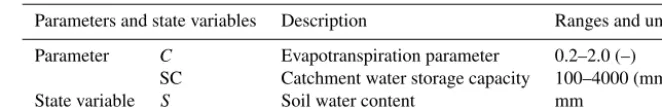
Table 1.States and parameters of the two-parameter monthly water balance model.
Parameters and state variables Description Ranges and unit
Parameter C Evapotranspiration parameter 0.2–2.0 (–) SC Catchment water storage capacity 100–4000 (mm) State variable S Soil water content mm
2014; Deng et al., 2015). Furthermore, the EnKF has been successfully used in time-invariant parameter estimations for hydrological models (Moradkhani et al., 2005; Wang et al., 2009; Xie and Zhang, 2010, 2013).
In this paper, the EnKF is applied to simultaneously esti-mate state variables and parameters (Table 1) in the TWBM model. The augmented state vector includes both states and model parameters (Wang et al., 2009), i.e., Z=(θ, x)T, whereθ includes the evapotranspiration parameter (C) and the catchment water storage capacity (SC), andxis the soil water content (S). The model forecast is conducted for each ensemble member as follows:
θik+1|i xik+1|i
!
=
θik|i fxik|i, θik+1|i, ui+1
!
+
δik εik
,
whereδki ∼N (0, Ui) , εik∼N (0, Gi) , (5) θik+1|i is thekth ensemble member forecast of model param-eters at timei+1;θik|i is thekth updated ensemble member of model parameters at time i; xik+1|i is the kth ensemble member forecast of model state at timei+1;xik|i is thekth updated ensemble member of model state at timei;f is the forecasting model operator, i.e., the TWBM model;ui+1is the forcing data for the hydrological model, including pre-cipitation and potential evapotranspiration;εki andδki are the independent white noise for the forecasting model, follow-ing a Gaussian distribution with zero mean and specified co-varianceGi andUi, respectively. Note that the parameters in Eq. (5) are propagated by adding random disturbances to the parameter member between time steps (Wang et al., 2009).
The observation ensemble member can be written as
yik+1=hxik+1|i, θik+1|i+ξik+1, ξik+1∼N (0, Wi+1) , (6) whereyik+1is thekth ensemble member of the model simu-lated runoff at timei+1;his the observation operator which represents the relationship between the observation and the state variables;ξik+1is the noise term, which follows a Gaus-sian distribution with zero mean and specified covariance
Wi+1.
Based on the available state and observation equations, the model parameters and state are updated according to the fol-lowing equation:
Zki+1|i+1=Zki+1|i +Ki+1
yki+1−hZik|i, (7)
whereZ is the augmented state vector that includes both states and parameters;yik+1 is thekth observation ensemble member generated by adding the observation errorξik+1 to the observed runoff:
yik+1=yi+1+ξik+1, (8)
Ki+1 is the Kalman gain matrix that represents the weight between the forecasts and observations. It can be calculated as (Evensen, 1994, 2003; Evensen and van Leeuwen, 1996; Moradkhani et al., 2005)
Ki+1= zy X
i+1|i yy X
i+1|i
+Wi+1
!−1
, (9)
wherePzy
i+1|i is the cross-covariance of the forecasted state and parameters and Pyy
i+1|i is the error covariance of the forecasted output. The error covariance matrix is calculated based on the forecasted ensemble members:
X
i+1|i
= 1
N−1Zi+1|iZ T
i+1|i, (10)
whereZi+1|i =
z1i+1|i −zi+1|i,· · ·, zNi+1|i −zi+1|i
;zi+1|i is the ensemble mean of the forecasted members, andN is the ensemble size.
that of SC is set to 5.0, 1.0 and 0.5 in the synthetic exper-iment, Wudinghe basin and Tongtianhe basin, respectively. The standard deviations of both model state and observation errors are assumed to be proportional to the magnitude of true values (Wang et al., 2009; Lü et al., 2013). The proportional factors of the model state are set to 0.05 for all the cases. Different proportional factors of runoff observation and pre-cipitation (Table 3) are evaluated to examine the capability of the EnKF in the synthetic experiment, whereas the pro-portional factors of runoff observation are set to 0.1 and zero precipitation errors are assumed in the two case studies. 2.3 Evaluation index
Two evaluation criteria, including the Nash–Sutcliffe effi-ciency (NSE) (Nash and Sutcliffe, 1970) and the volume er-ror (VE) are used to evaluate the runoff assimilation results for the synthetic experiment and the application to real catch-ments (Deng et al., 2015; Li et al., 2015).
NSE=1−
Pn
i=1 Qsim,i−Qobs,i 2
Pn
i=1 Qobs,i−Qobs
2 , (11)
VE=
Pn
i=1Qsim,i−Pni=1Qobs,i Pn
i=1Qobs,i
, (12)
where Qsim,i and Qobs,i are the simulated and observed runoff for theith month,Qobsis the mean value of the ob-served runoff and nis the total number of data points. The NSE ranges from−∞to 1 and has been widely used to as-sess the goodness of fit for hydrological modeling. A NSE value of 1 stands for a perfect match of simulated runoff to the observations, whereas a value of 0 indicates that the model simulations are equivalent to the mean value of the runoff observations; negative NSE values indicate that the mean observed runoff is better than the model simulations. The VE is a measure of bias between the simulated and ob-served runoff. For example, VE with the value of 0 denotes no bias, and a negative value means an underestimation of the total runoff volume.
The assimilated parameter results are evaluated using the following criteria, including the Pearson correlation coeffi-cient (R), the root mean square error (RMSE) and mean ab-solute relative error (MARE):
R=
Pn
i=1 θsim,i−θsim
θobs,i−θobs
q Pn
i=1 θsim,i−θsim 2
θobs,i−θobs
2, (13)
RMSE=
r
1
n Xn
i=1 θsim,i−θobs,i
2
, (14)
MARE=1
n Xn
i=1
θsim,i−θobs,i
θobs,i
, (15)
whereθsim,iandθobs,i are the assimilated and true model pa-rameters for theith month,θsimandθobsare the mean of the assimilated and true model parameters for theith month and
nis the total number of data points.
3 Data and study area 3.1 Synthetic experiment
A synthetic experiment is designed to evaluate the capability of the assimilation procedure to identify the temporal vari-ation of model parameters. Five scenarios of different pa-rameter variations are developed, as shown in Table 2. The model parameters in the first four scenarios are time variant, and those in the last scenario are constant. ParameterC, the evapotranspiration parameter, is considered to be sinusoidal reflecting potential seasonal variations in hydrological model parameters (Paik et al., 2005; Ye et al., 1997). An increasing trend is also considered to account for the potential annual or long-term variability. The change of parameter SC is con-sidered to be gradual and abrupt, since the catchment water storage capacity can be affected by land use and land cover changes, such as afforestation and dam construction. The pa-rameters in scenario 5 are treated as constants like in conven-tional hydrological modeling. Observations for precipitation and potential evapotranspiration are generated by adding a Gaussian disturbance to the corresponding data from a real catchment, and runoff is then produced using the TWBM model. The data set used in this experiment is 672 months long. The first 24-month period is set for model warm-up to reduce the impact of the initial soil moisture conditions. The steps toward identifying temporal variation of model param-eters are as follows:
1. Time series of model parameters are synthetically gen-erated, including the time-variant parameters and the constant parameters. Model parameter sets are produced using a sinusoidal function and/or a linear trend function within the specified ranges shown in Table 1. The runoff observations for each scenario are computed from the TWBM model taking monthly potential evapotranspira-tion, monthly precipitation and the parameters as inputs. 2. The initial ensembles of model parameters and state variables are generated using uniform distributions within the specified ranges in Table 1. The ensemble size and the total number of assimilation time steps are specified.
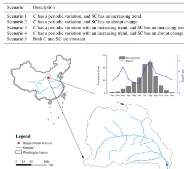
Table 2.Different variations of model parameters in the synthetic experiment.
Scenario Description
Scenario 1 Chas a periodic variation, and SC has an increasing trend Scenario 2 Chas a periodic variation, and SC has an abrupt change
Scenario 3 Chas a periodic variation with an increasing trend, and SC has an increasing trend Scenario 4 Chas a periodic variation with an increasing trend, and SC has an abrupt change Scenario 5 BothCand SC are constant
[image:5.612.74.261.489.534.2]Figure 1.Location and mean monthly precipitation and runoff from 1956 to 2000 of the Wudinghe basin.
Table 3.Proportional factors of the standard deviations for precipi-tation (γP)and runoff (γQ)uncertainties.
Type Low level Medium level High level
γP 0 0.05 0.10
γQ 0.05 0.10 0.20
deviations are assumed to be proportional to the magnitude of the true values, and the corresponding proportional fac-tors are denoted asγP andγQ. The proportional factors are set to account for the practical measurement error (Wang et al., 2009; Xie and Zhang, 2010).
3.2 Study area
3.2.1 Case 1: Wudinghe basin
The method is applied to the Wudinghe basin (Fig. 1), which is a sub-basin of the Yellow River basin and located in the southern fringe of the Maowusu Desert and the northern part of the Loess Plateau in China, where the climate is semiarid
climate. It has a drainage area of approximately 30 261 km2 and a total length of 491 km. The Wudinghe basin has an average slope of 0.2 %, and its elevation ranges from 600 to 1800 m above the sea level. The Baijiachuan gauge sta-tion, which is the most downstream station of the Wudinghe basin, drains 98 % of the total basin area. The mean annual precipitation over the basin is 401 mm, of which 72.5 % oc-curs in the rainy season from June to September (Fig. 2). The mean annual potential evapotranspiration is 1077 mm, and the mean annual runoff is about 39 mm with a runoff coeffi-cient of 0.1.
Figure 2.Location and mean monthly precipitation and runoff from 1980 to 2013 of the Tongtianhe basin.
Figure 3.Comparison between estimatedCand its true values for various parameter changes under different uncertainty levels. The gray areas represent the 95 % prediction uncertainty intervals.
3.2.2 Case 2: Tongtianhe basin
The Tongtianhe basin (Fig. 3) is located in the southwestern Qinghai Province, China, with a continental climate. It be-longs to the source area of the Yangtze River basin with a drainage area of about 140 000 km2and a total main stream
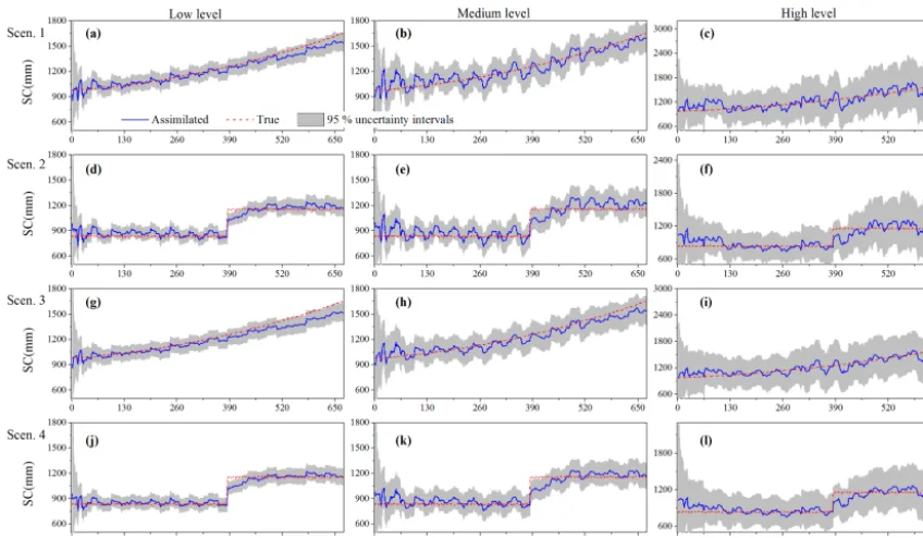
[image:6.612.88.510.336.588.2]Figure 4.Comparison between estimated SC and its true values for various parameter changes under different uncertainty levels. The gray areas represent the 95 % prediction uncertainty intervals.
99 mm with a runoff coefficient of 0.23. The Tongtianhe basin is rarely affected by human activities, owing to the water source protection guidelines conducted by the govern-ment. The Tongtianhe basin is used for comparison on model parameter identification.
3.2.3 Data
The data sets used in this study include monthly precipi-tation, potential evapotranspiration and runoff in the Wud-inghe basin (from 1956 to 2000) and the Tongtianhe basin (from 1980 to 2013). The potential evapotranspiration is es-timated using the Penman–Monteith equation (Allen et al., 1998) based on the meteorological data from the China Mete-orological Data Sharing Service System (http://data.cma.cn). To reduce the impact of the initial conditions, a 2-year data set, i.e., from 1956 to 1957 for Wudinghe basin and from 1980 to 1981 for Tongtianhe basin, is reserved as the warm-up period.
4 Results and discussion 4.1 Synthetic experiment
The comparisons of the estimated and true model parameters under different scenarios are presented in Figs. 3, 4 and 5. Tables 4 and 5 show the evaluated statistics for the parame-ters and runoff estimations. The assimilated parameter values are obtained from the ensemble mean at each time step. The
estimation of parametersC and SC have the similar trends to the true parameter series. The temporal variations of the estimatedC agree well with the true series, although it has biases on the peaks of the periodic changes. For SC, the tem-poral estimates can capture the different changes in Table 2, especially for the abrupt change where the estimated values respond immediately. Different uncertainty levels are consid-ered to examine the capability of the EnKF method. The re-sults in Fig. 3 show that the estimatedChas more accurate peaks with smaller RMSE and higher R values under the high-level uncertainty (Table 4); whereas, the SC estimates in Fig. 4 have some fluctuations when the uncertainty level increases. This is due to the estimated values vary with in-creasing uncertainty levels in the assimilation process. In the synthetic experiment, the trueC is assumed to be periodic with a higher degree of variation, whereas the true SC series have less variation.
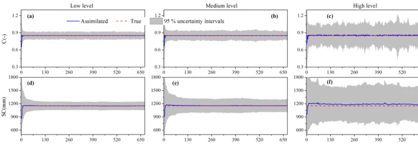
be-Figure 5.Estimations of time-invariantCand SC under different uncertainty levels. The gray areas represent the 95 % prediction uncertainty intervals.
Table 4.Performance statistics for various changes of(a)parameterCand(b)SC estimations under different levels of uncertainty in the synthetic experiment.
Scenario Low level Medium level High level
RMSE MARE R RMSE MARE R RMSE MARE R
(a)ParameterC
Scenario 1 0.15 0.21 0.55 0.16 0.18 0.68 0.18 0.11 0.89 Scenario 2 0.16 0.19 0.63 0.17 0.16 0.75 0.18 0.09 0.91 Scenario 3 0.12 0.13 0.64 0.13 0.11 0.72 0.14 0.07 0.91 Scenario 4 0.13 0.12 0.70 0.13 0.10 0.77 0.14 0.06 0.93
Scenario 5 0 – – 0 – – 0 – –
(b)Parameter SC
Scenario 1 182.87 0.03 0.99 187.76 0.05 0.94 253.35 0.83 0.83 Scenario 2 158.30 0.04 0.96 167.47 0.07 0.91 189.59 0.80 0.80 Scenario 3 180.20 0.03 0.99 183.06 0.04 0.97 215.04 0.88 0.88 Scenario 4 156.42 0.03 0.97 158.50 0.05 0.93 170.90 0.86 0.86
Scenario 5 1.54 – – 3.67 – – 20.54 – –
tween assimilated and true values exists particularly when peak values occur (Clark et al., 2008; Samuel et al., 2014).
The results for the scenario of constant parameters are shown in Fig. 5, demonstrating that the estimated parame-ters can approach their true values after the initial 24 assim-ilation steps. The gray areas represent the 95 % prediction uncertainty intervals, which reduce quickly and approach a stable spread. The performance of the estimated parame-ters is correlated with the uncertainty level. Higher precipita-tion and runoff observaprecipita-tion errors correspond to the greater RMSE values (Table 4) of estimated parameters and un-certainty ranges. The performance of runoff estimations for various parameter changes under different levels of uncer-tainty is shown in Table 5, suggesting that the EnKF per-fectly matches the observations with NSEs higher than 0.95 and absolute VEs smaller than 0.02. The EnKF can success-fully capture the temporal variations of the true parameters, although the uncertainty levels of the observations can affect
its performance to a certain degree. The above results demon-strate that the EnKF is able to identify the temporal variation of the model parameters by updating the state variables and parameters based on the runoff observations.
4.2 Case studies
[image:8.612.108.487.290.482.2]Table 5.Performance of runoff estimations for various parameter changes under different levels of uncertainty in the synthetic experiment.
Scenario Low level Medium level High level
NSE VE NSE VE NSE VE
[image:9.612.46.288.206.405.2]Scenario 1 0.999 −0.0003 0.988 −0.0046 0.967 −0.0230 Scenario 2 0.999 0.0001 0.990 −0.0028 0.967 −0.0141 Scenario 3 0.999 −0.0011 0.990 −0.0013 0.974 −0.0264 Scenario 4 0.999 −0.0009 0.992 0.0002 0.959 −0.0147 Scenario 5 0.999 −0.0022 0.992 −0.0077 0.961 −0.0187
Figure 6.Double mass curve between monthly runoff and precipi-tation for Wudinghe basin within the period of 1958–2000(a)and Tongtianhe basin within the period of 1982–2013(b).
a single linear relationship fits all the data for the Tongtianhe basin, suggesting a stable precipitation–runoff relationship during the 1982–2013 period.
The estimated parameters and the associated 95 % predic-tion uncertainty intervals are shown in Fig. 7. The time series of estimated SC shows an apparent increasing trend, with two different trends for pre- and post-turning points in Fig. 6a. The temporal variation of the water storage capacity is cor-related with the changes of land use and land cover. Both the trends in Fig. 7c show an increase of SC because the im-plementation of the large-scale engineering measures signifi-cantly improved the water holding capacity of the Wudinghe basin, especially for the reservoir and check dam construc-tion. The trend slopes of the two periods, one from 1956 to 1971 and the other from 1972 to 2000, are different because the degree of implementing engineering measures varied dur-ing the period of 1958–2000. Moreover, the increase of the water holding capacity slowed down during the 1980s due to the sedimentation in reservoirs and check dams after peri-ods of operation (Wang and Fan, 2003). Figure 8a shows the
long-term time series of precipitation and potential evapora-tion in the Wudinghe basin. The result shows that the runoff decreases significantly while precipitation changes slightly and potential evaporation has no trend, indicating that the actual evaporation increases significantly due to impacts of human activities, i.e., soil and water conservation measures. Figure 8b presents the runoff reduction caused by all the soil and water conservation measures, i.e., land terracing, tree and grass plantation and check dam and reservoir construction. The runoff reduction positively relates to the water holding capacity, namely the SC value. The slope for the period of 1958–1971 is higher than that for the period of 1972–1996, suggesting that the SC in the former period has a higher in-creasing trend. On the other hand, results of Tongtianhe basin show that the estimated SC has no detectable trend with a smallRvalue. Moreover, the ranges and standard deviation of the estimated SC values are much smaller than those in the Wudinghe basin (Fig. 7), suggesting that the estimated SC has no obvious temporal variations.
For parameterC, the results show that the estimates have no significant temporal patterns because the trend line slopes are almost zero and the standard deviations are relatively small for the two basins (Fig. 7a and b); however, it can be treated as a time-variant parameter since temporal variations exist in the estimatedC series. The temporal variations of the estimatedCare related to the variation of monthly actual evaporation, which is affected by multiple climatic factors, such as air temperature, soil moisture and solar irradiance (Su et al., 2015). The gray regions represent the 95 % pre-diction uncertainty intervals obtained from the parameter en-sembles. The stable and narrow uncertainty bounds shown in Fig. 7 indicate that the EnKF can provide superior perfor-mance of parameter estimation. The runoff simulations for both basins match well with the runoff observations. Specif-ically, the NSE and VE for the Wudinghe basin are 0.93 and 0.07, respectively. While the corresponding index values for the Tongtianhe basin are 0.99 and 0.04.
Figure 7.Estimated parameter values ofCand SC for (1) Wudinghe basin within the period of 1958–2000, and (2) Tongtianhe basin within the period of 1982–2013. The gray areas represent the 95 % prediction uncertainty intervals. Note that the MSE denotes the standard deviation of the estimated parameter values.
Figure 8. (a)Yearly precipitation, potential evaporation and runoff in Wudinghe basin during the period of 1958–2000;(b)Runoff re-duction in Wudinghe basin caused by all the soil and water conser-vation measures, i.e., land terracing, tree and grass plantation and check dam and reservoir construction for the period of 1958–1996. Note that the data are from Wang and Fan (2003) and are only avail-able from 1956 to 1996.
the estimated SC for the Tongtianhe basin is approximately stable with a small standard deviation because the basin is located in a water protection zone and has no significant changes on water storage capacity caused by human activ-ities. The parameter C has temporal variations and can be treated as a time-variant parameter for both basins, although the estimates have no obvious temporal patterns. Therefore,
the EnKF is capable of identifying the temporal variations of model parameters.
5 Conclusions
This study proposes an ensemble Kalman filter (EnKF) to identify the temporal variation of model parameters of the two-parameter monthly water balance model (TWBM) by assimilating runoff observations. A synthetic experiment, which contains four scenarios with different changes of model parameters and one scenario with constant parame-ters, is designed to examine the capability of the proposed approach. Furthermore, three different levels of observation uncertainty are taken to assess the performance of the EnKF. The main conclusions are as follows. For the time-variant parameters, the EnKF provides superior performance even though slight time lags exist for parameters with periodic variations. The true values of the constant parameters can be approached quickly after 24 time steps of the assimila-tion process. The temporal variaassimila-tions of the parameters can be successfully captured even under a high level of obser-vation uncertainties, which would have an influence on the performance of the EnKF.
[image:10.612.47.285.330.526.2]period of 1958–2000 in the Wudinghe basin. The soil and water conservation measures, including land terracing, tree and grass plantation and check dam and reservoir construc-tion, were implemented from 1958 to 2000, resulting in the increase of the water holding capacity of the basin, which ex-plains the increasing trend of SC. Moreover, the magnitudes of the engineering measures in different time periods play an important role in the degree of increasing trend for SC. In the Tongtianhe basin, the parameter SC has no significant trend for the period of 1982–2013, which is consistent with the relatively stationary catchment characteristics. The evap-otranspiration parameter (C) has temporal variations and can be treated as a time-variant parameter, but no obvious trends exist.
The method proposed in this paper provides an effective tool for the time-variant model parameter identification. Fu-ture work will be focused on the influence of the correlations between/among model parameters and performance compar-ison of multiple data assimilation methods.
6 Data availability
The meteorological data can be requested and obtained from the China Meteorological Data Sharing Service System (http: //data.cma.cn). According to the website’s data sharing rules, data sets from the website cannot be uploaded or shared per-sonally. However, readers can access the data themselves through registration. Note that the runoff data from the local hydrology bureau is also not publicly accessible. The hydro-logical data, including the precipitation and runoff records, are managed by local Hydrology and Water Resources Bu-reau of China.
Acknowledgements. This study was supported by the Excel-lent Young Scientist Foundation of NSFC (51422907) and the Open Foundation of State Key Laboratory of Water Resources and Hydropower Engineering Science in Wuhan University (2015SWG01). The authors thank the China Meteorological Data Sharing Service System for providing part of the data used in this study. The authors would like to thank the editor and the anonymous reviewers for their comments that helped to improve the quality of the paper.
Edited by: A. Guadagnini
Reviewed by: two anonymous referees
References
Abaza, M., Anctil, F., Fortin, V., and Turcotte, R.: Se-quential streamflow assimilation for short-term hydrolog-ical ensemble forecasting, J. Hydrol., 519, 2692–2706, doi:10.1016/j.jhydrol.2014.08.038, 2014.
Allen, R. G., Pereira, L. S., Raes, D., and Smith, M.: Crop Evapotranspiration-Guidelines for Computing Crop
Wa-ter Requirements-FAO Irrigation and Drainage Paper 56, Food and Agriculture Organization of the United Nations, Rome, Italy, 1998.
Andréassian, V., Parent, E., and Michel, C.: A distribution-free test to detect gradual changes in watershed behavior, Water Resour. Res., 39, 1252, doi:10.1029/2003WR002081, 2003.
Brigode, P., Oudin, L., and Perrin, C.: Hydrological model parame-ter instability: A source of additional uncertainty in estimating the hydrological impacts of climate change?, J. Hydrol., 476, 410–425, doi:10.1016/j.jhydrol.2012.11.012, 2013.
Brown, A. E., Zhang, L., McMahon, T. A., Western, A. W., and Vertessy, R. A.: A review of paired catch-ment studies for determining changes in water yield result-ing from alterations in vegetation, J. Hydrol., 310, 28–61, doi:10.1016/j.jhydrol.2004.12.010, 2005.
Burgers, G., van Leeuwen, P. J., and Evensen, G.: Anal-ysis scheme in the ensemble Kalman filter, Mon. Weather Rev., 126, 1719–1724, doi:10.1175/1520-0493(1998)126<1719:ASITEK>2.0.CO;2, 1998.
Clark, M. P., Rupp, D. E., Woods, R. A., Zheng, X., Ibbitt, R. P., Slater, A. G., Schmidt, J., and Uddstrom, M. J.: Hy-drological data assimilation with the ensemble Kalman fil-ter: Use of streamflow observations to update states in a dis-tributed hydrological model, Adv. Water Resour., 31, 1309– 1324, doi:10.1016/j.advwatres.2008.06.005, 2008.
Coron, L., Andréassian, V., Perrin, C., Lerat, J., Vaze, J., Bourqui, M., and Hendrickx, F.: Crash testing hydrological models in contrasted climate conditions: An experiment on 216 Australian catchments, Water Resour. Res., 48, W05552, doi:10.1029/2011WR011721, 2012.
DeChant, C. M. and Moradkhani, H.: Toward a reliable predic-tion of seasonal forecast uncertainty: Addressing model and ini-tial condition uncertainty with ensemble data assimilation and sequential Bayesian combination, J. Hydrol., 519, 2967–2977, doi:10.1016/j.jhydrol.2014.05.045, 2014.
Delijani, E. B., Pishvaie, M. R., and Boozarjomehry, R. B.: Subsur-face characterization with localized ensemble Kalman filter em-ploying adaptive thresholding, Adv. Water Resour., 69, 181–196, doi:10.1016/j.advwatres.2014.04.011, 2014.
Deng, C., Liu, P., Guo, S., Wang, H., and Wang, D.: Estimation of nonfluctuating reservoir inflow from water level observations using methods based on flow continuity, J. Hydrol., 529, 1198– 1210, doi:10.1016/j.jhydrol.2015.09.037, 2015a.
Deng, C., Liu, P., Liu, Y., Wu, Z. H., and Wang, D.: In-tegrated hydrologic and reservoir routing model for real-time water level forecasts, J. Hydrol. Eng., 20, 05014032, doi:10.1061/(ASCE)HE.1943-5584.0001138, 2015b.
Evensen, G.: Sequential data assimilation with a nonlinear quasi-geostrophic model using Monte Carlo methods to fore-cast error statistics, J. Geophys. Res., 99, 10143–10162, doi:10.1029/94JC00572, 1994.
Evensen, G.: The Ensemble Kalman filter: theoretical formula-tion and practical implementaformula-tion, Ocean Dynam., 53, 343–367, doi:10.1007/s10236-003-0036-9, 2003.
Guo, S., Wang, J., Xiong, L., Ying, A., and Li, D.: A macro-scale and semi-distributed monthly water balance model to pre-dict climate change impacts in China, J. Hydrol., 268, 1–15, doi:10.1016/S0022-1694(02)00075-6, 2002.
Guo, S., Chen, H., Zhang, H., Xiong, L., Liu, P., Pang, B., Wang, G., and Wang, Y.: A semi-distributed monthly water balance model and its application in a climate change impact study in the middle and lower Yellow River basin, Water Int., 30, 250–260, doi:10.1080/02508060508691864, 2005.
Han, E., Merwade, V., and Heathman, G. C.: Implementation of surface soil moisture data assimilation with watershed scale distributed hydrological model, J. Hydrol., 416–417, 98–117, doi:10.1016/j.jhydrol.2011.11.039, 2012.
Jeremiah, E., Marshall, L., Sisson, S. A., and Sharma, A.: Speci-fying a hierarchical mixture of experts for hydrologic modeling: Gating function variable selection, Water Resour. Res., 49, 2926– 2939, doi:10.1002/wrcr.20150, 2013.
Kumar, S. V., Reichle, R. H., Harrison, K. W., Peters-Lidard, C. D., Yatheendradas, S., and Santanello, J. A.: A comparison of meth-ods for a priori bias correction in soil moisture data assimilation, Water Resour. Res., 48, W03515, doi:10.1029/2010WR010261, 2012.
Kurtz, W., Hendricks Franssen, H.-J., and Vereecken, H.: Idtification of time-variant river bed properties with the en-semble Kalman filter, Water Resour. Res., 48, W10534, doi:10.1029/2011WR011743, 2012.
Li, S., Xiong, L., Dong, L., and Zhang, J.: Effects of the Three Gorges Reservoir on the hydrological droughts at the down-stream Yichang station during 2003–2011, Hydrol. Process., 27, 3981–3993, doi:10.1002/hyp.9541, 2013.
Li, X.-N., Xie, P., Li, B.-B., and Zhang, B.: A probabil-ity calculation method for different grade drought event un-der changing environment-Taking Wuding River basin as an example, Shuili Xuebao, J. Hydraul. Eng., 45, 585–594, doi:10.13243/j.cnki.slxb.2014.05.010, 2014 (in Chinese). Li, Y., Ryu, D., Western, A. W., and Wang, Q. J.: Assimilation of
stream discharge for flood forecasting: The benefits of account-ing for routaccount-ing time lags, Water Resour. Res., 49, 1887–1900, doi:10.1002/wrcr.20169, 2013.
Li, Z., Liu, P., Deng, C., Guo, S., He, P., and Wang, C.: Evalu-ation of the estimEvalu-ation of distribution algorithm to calibrate a computationally intensive hydrologic model, J. Hydrol. Eng., 21, 04016012, doi:10.1061/(ASCE)HE.1943-5584.0001350, 2015. Liu, Y. and Gupta, H. V.: Uncertainty in hydrologic modeling:
To-ward an integrated data assimilation framework, Water Resour. Res., 43, 1–18, doi:10.1029/2006WR005756, 2007.
Liu, Y., Weerts, A. H., Clark, M., Hendricks Franssen, H.-J., Kumar, S., Moradkhani, H., Seo, D.-J., Schwanenberg, D., Smith, P., van Dijk, A. I. J. M., van Velzen, N., He, M., Lee, H., Noh, S. J., Rakovec, O., and Restrepo, P.: Advancing data assimilation in operational hydrologic forecasting: progresses, challenges, and emerging opportunities, Hydrol. Earth Syst. Sci., 16, 3863–3887, doi:10.5194/hess-16-3863-2012, 2012.
Lü, H. S., Hou, T., Horton, R., Zhu, Y. H., Chen, X., Jia, Y. W., Wang, W., and Fu, X. L.: The streamflow estima-tion using the Xinanjiang rainfall runoff model and dual state-parameter estimation method, J. Hydrol., 480, 102–114, doi:10.1016/j.jhydrol.2012.12.011, 2013.
Merz, R., Parajka, J., and Blöschl, G.: Time stability of catchment model parameters: Implications for climate impact analyses, Water Resour. Res., 47, W02531, doi:10.1029/2010WR009505, 2011.
Montzka, C., Grant, J. P., Moradkhani, H., Franssen, H.-J. H., Wei-hermüller, L., Drusch, M., and Vereecken, H.: Estimation of radiative transfer parameters from L-band passive microwave brightness temperatures using advanced data assimilation, Va-dose Zone J., 12, 1–17, doi:10.2136/vzj2012.0040, 2013. Moradkhani, H., Sorooshian, S., Gupta, H. V., and Houser, P.
R.: Dual state–parameter estimation of hydrological models us-ing ensemble Kalman filter, Adv. Water Resour., 28, 135–147, doi:10.1016/j.advwatres.2004.09.002, 2005.
Nash, J. E. and Sutcliffe, J. V.: River flow forecasting through con-ceptual models part I: A discussion of principles, J. Hydrol., 10, 282–290, doi:10.1016/0022-1694(70)90255-6, 1970.
Nie, S., Zhu, J., and Luo, Y.: Simultaneous estimation of land sur-face scheme states and parameters using the ensemble Kalman filter: identical twin experiments, Hydrol. Earth Syst. Sci., 15, 2437–2457, doi:10.5194/hess-15-2437-2011, 2011.
Paik, K., Kim, J. H., Kim, H. S., and Lee, D. R.: A concep-tual rainfall-runoff model considering seasonal variation, Hydrol. Process., 19, 3837–3850, doi:10.1002/hyp.5984, 2005.
Panzeri, M., Riva, M., Guadagnini, A., and Neuman, S. P.: Data assimilation and parameter estimation via ensemble Kalman filter coupled with stochastic moment equations of tran-sient groundwater flow, Water Resour. Res., 49, 1334–1344, doi:10.1002/wrcr.20113, 2013.
Patil, S. D. and Stieglitz, M.: Comparing spatial and temporal trans-ferability of hydrological model parameters, J. Hydrol., 525, 409–417, doi:10.1016/j.jhydrol.2015.04.003, 2015.
Pauwels, V. R. N. and Lannoy, G. J. M. D.: Improvement of Mod-eled Soil Wetness Conditions and Turbulent Fluxes through the Assimilation of Observed Discharge, J. Hydrometeorol., 7, 458– 477, doi:10.1175/JHM490.1, 2006.
Peel, M. C. and Blöschl, G.: Hydrological modelling in a changing world, Prog. Phys. Geog., 35, 249–261, doi:10.1177/0309133311402550, 2011.
Samuel, J., Coulibaly, P., Dumedah, G., and Moradkhani, H.: Assessing model state and forecasts variation in hy-drologic data assimilation, J. Hydrol., 513, 127–141, doi:10.1016/j.jhydrol.2014.03.048, 2014.
Seiller, G., Anctil, F., and Perrin, C.: Multimodel evaluation of twenty lumped hydrological models under contrasted cli-mate conditions, Hydrol. Earth Syst. Sci., 16, 1171–1189, doi:10.5194/hess-16-1171-2012, 2012.
Shi, Y., Davis, K. J., Zhang, F., Duffy, C. J., and Yu, X.: Parameter estimation of a physically based land surface hydrologic model using the ensemble Kalman filter: A synthetic experiment, Water Resour. Res., 50, 706–724, doi:10.1002/2013WR014070, 2014. Su, T., Feng, T., and Feng, G.: Evaporation variability under climate
warming in five reanalyses and its association with pan evap-oration over China, J. Geophys. Res.-Atmos., 120, 8080–8098, doi:10.1002/2014JD023040, 2015.
Thirel, G., Andréassian, V., Perrin, C., Audouy, J. N., Berthet, L., Edwards, P., Folton, N., Furusho, C., Kuentz, A., Lerat, J., Lindström, G., Martin, E., Mathevet, T., Merz, R., Parajka, J., Ruelland, D., and Vaze, J.: Hydrology under change: an eval-uation protocol to investigate how hydrological models deal with changing catchments, Hydrolog. Sci. J., 60, 1184–1199, doi:10.1080/02626667.2014.967248, 2015.
Vrugt, J. A., ter Braak, C. J. F., Diks, C. G. H., and Schoups, G.: Hydrologic data assimilation using particle Markov chain Monte Carlo simulation: Theory, concepts and applications, Adv. Wa-ter Resour., 51, 457–478, doi:10.1016/j.advwatres.2012.04.002, 2013.
Wang, D., Chen, Y., and Cai, X.: State and parameter estimation of hydrologic models using the constrained ensemble Kalman filter, Water Resour. Res., 45, W11416, doi:10.1029/2008WR007401, 2009.
Wang, G. and Fan, Z.: A study of water and sediment changes in the Yellow River, Publishing House of Yellow River Water Conser-vancy, Zhengzhou, China, 2003 (in Chinese).
Weerts, A. H. and El Serafy, G. Y. H.: Particle filtering and ensem-ble Kalman filtering for state updating with hydrological con-ceptual rainfall-runoff models, Water Resour. Res., 42, 1–17, doi:10.1029/2005WR004093, 2006.
Westra, S., Thyer, M., Leonard, M., Kavetski, D., and Lam-bert, M.: A strategy for diagnosing and interpreting hydrologi-cal model nonstationarity, Water Resour. Res., 50, 5090–5113, doi:10.1002/2013WR014719, 2014.
Xie, X. and Zhang, D.: Data assimilation for distributed hydrolog-ical catchment modeling via ensemble Kalman filter, Adv. Wa-ter Resour., 33, 678–690, doi:10.1016/j.advwatres.2010.03.012, 2010.
Xie, X. and Zhang, D.: A partitioned update scheme for state-parameter estimation of distributed hydrologic models based on the ensemble Kalman filter, Water Resour. Res., 49, 7350–7365, doi:10.1002/2012WR012853, 2013.
Xie, X., Meng, S., Liang, S., and Yao, Y.: Improving streamflow predictions at ungauged locations with real-time updating: ap-plication of an EnKF-based state-parameter estimation strategy, Hydrol. Earth Syst. Sci., 18, 3923–3936, doi:10.5194/hess-18-3923-2014, 2014.
Xiong, L. and Guo, S.: A two-parameter monthly water bal-ance model and its application, J. Hydrol., 216, 111–123, doi:10.1016/S0022-1694(98)00297-2, 1999.
Xiong, L. and Guo, S.: Appraisal of Budyko formula in calculating long-term water balance in humid watersheds of southern China, Hydrol. Process., 26, 1370–1378, doi:10.1002/hyp.8273, 2012. Xiong, L., Yu, K.-X., and Gottschalk, L.: Estimation of the
distribu-tion of annual runoff from climatic variables using copulas, Wa-ter Resour. Res., 50, 7134–7152, doi:10.1002/2013WR015159, 2014.
Xu, J.: Variation in annual runoff of the Wudinghe River as influ-enced by climate change and human activity, Quatern. Int., 244, 230–237, doi:10.1016/j.quaint.2010.09.014, 2011.
Xue, L. and Zhang, D.: A multimodel data assimilation framework via the ensemble Kalman filter, Water Resour. Res., 50, 4197– 4219, doi:10.1002/2013WR014525, 2014.
Yan, H., DeChant, C. M., and Moradkhani, H.: Improving soil moisture profile prediction with the particle filter-Markov chain Monte Marlo method, IEEE T. Geosci. Remote, 53, 6134–6147, doi:10.1109/tgrs.2015.2432067, 2015.
Ye, W., Bates, B. C., Viney, N. R., Sivapalan, M., and Jakeman, A. J.: Performance of conceptual rainfall-runoff models in low-yielding ephemeral catchments, Water Resour. Res., 33, 153– 166, doi:10.1029/96WR02840, 1997.
Zhang, D., Liu, X. M., Liu, C. M., and Bai, P.: Responses of runoff to climatic variation and human activities in the Fenhe River, China, Stoch. Env. Res. Risk A., 27, 1293–1301, doi:10.1007/s00477-012-0665-y, 2013.