https://doi.org/10.5194/hess-22-6187-2018 © Author(s) 2018. This work is distributed under the Creative Commons Attribution 4.0 License.
Analysis of combined and isolated effects of land-use
and land-cover changes and climate change on the
upper Blue Nile River basin’s streamflow
Dagnenet Fenta Mekonnen1,2, Zheng Duan1, Tom Rientjes3, and Markus Disse1
1Chair of Hydrology and River Basin Management, Faculty of Civil, Geo and Environmental Engineering,
Technische Universität München, Arcisstrasse 21, 80333, Munich, Germany
2Amhara Regional State Water, Irrigation and Energy Development Bureau, Bahir Dar, Ethiopia 3Department of Water Resources, Faculty of Geo-information Science and Earth Observation (ITC),
University of Twente, Enschede, the Netherlands
Correspondence:Dagnenet Fenta Mekonnen ([email protected]) Received: 23 November 2017 – Discussion started: 19 December 2017
Revised: 18 October 2018 – Accepted: 28 October 2018 – Published: 30 November 2018
Abstract. Understanding responses by changes in land use and land cover (LULC) and climate over the past decades on streamflow in the upper Blue Nile River basin is impor-tant for water management and water resource planning in the Nile basin at large. This study assesses the long-term trends of rainfall and streamflow and analyses the responses of steamflow to changes in LULC and climate in the upper Blue Nile River basin. Findings of the Mann–Kendall (MK) test indicate statistically insignificant increasing trends for basin-wide annual, monthly, and long rainy-season rainfall but no trend for the daily, short rainy-season, and dry sea-son rainfall. The Pettitt test did not detect any jump point in basin-wide rainfall series, except for daily time series rain-fall. The findings of the MK test for daily, monthly, annual, and seasonal streamflow showed a statistically significant increasing trend. Landsat satellite images for 1973, 1985, 1995, and 2010 were used for LULC change-detection anal-ysis. The LULC change-detection findings indicate increases in cultivated land and decreases in forest coverage prior to 1995, but forest area increases after 1995 with the area of cultivated land that decreased. Statistically, forest coverage changed from 17.4 % to 14.4%, by 12.2 %, and by 15.6 %, while cultivated land changed from 62.9 % to 65.6 %, by 67.5 %, and by 63.9 % from 1973 to 1985, in 1995, and in 2010, respectively. Results of hydrological modelling indi-cate that mean annual streamflow increased by 16.9 % be-tween the 1970s and 2000s due to the combined effects of LULC and climate change. Findings on the effects of LULC
change on only streamflow indicate that surface runoff and base flow are affected and are attributed to the 5.1 % re-duction in forest coverage and a 4.6 % increase in cultivated land areas. The effects of climate change only revealed that the increased rainfall intensity and number of extreme rain-fall events from 1971 to 2010 significantly affected the sur-face runoff and base flow. Hydrological impacts by climate change are more significant as compared to the impacts of LULC change for streamflow of the upper Blue Nile River basin.
1 Introduction
varia-tions in climate, altitude and topography, and land-use and land-cover (LULC) change. Over the past decades, changes in climate (e.g. Haile et al., 2017) and changes in LULC (e.g. Woldesenbet et al., 2017b) have affected the magnitude of streamflow. Effective planning, management, and the reg-ulation of water resource development is therefore required to avert conflicts between the competing water users.
Only the understanding of the hydrological processes and sources impacting water quantity, such as LULC change and climate change, can achieve this, as they are the key driv-ing forces that can modify the watershed’s hydrology and water availability (Oki and Kanae, 2006; Woldesenbet et al., 2017b; Yin et al., 2017). LULC change can modify the rain-fall path to generate basin runoff by altering critical water-balance components, such as groundwater recharge, infiltra-tion, intercepinfiltra-tion, and evaporation. McCartney et al. (2012) and Alemseged and Tom (2015) described that the UBNRB experiences significant spatial and temporal climate variabil-ity. Less than 500 mm of precipitation falls annually near the Sudanese border, whereas more than 2000 mm falls annually in some areas of the southern basin (Awulachew et al., 2009). Potential evapotranspiration (ET) also varies considerably and is strongly correlated with altitude. At annual bases, it varies from more than 2200 mm near the Sudanese border to between about 1300 and 1700 mm in the Ethiopian highlands (McCartney et al., 2012). The precipitation and ET cycles are characterised by seasonal and inter-annual variability, which affect the characteristics of the UBNRB streamflow.
A literature review shows that several sub-basin or basin level studies were conducted in the UBNRB. Most of the studies focused on the trend analysis of precipitation and streamflow (see Bewket and Sterk, 2005; Cheung et al., 2008; Conway, 2000; Gebremicael et al., 2013; Melesse et al., 2009; Rientjes et al., 2011; Seleshi and Zanke, 2004; Teferi et al., 2013; Tekleab et al., 2014; Tesemma et al., 2010), and all reported no significant trend in annual and seasonal precipitation totals within the Lake Tana sub-basin, whereas Mengistu et al. (2014) reported statistically non-significant increasing trends in annual and seasonal rainfall series, ex-cept for a short rainy season (Belg) from February to May.
Gebremicael et al. (2013) reported statistically significant increasing long-term annual streamflow (1970–2005) at the El Diem gauging station for the UBNRB’s streamflow. How-ever, Tesemma et al. (2010) reported no statistically signif-icant trend for long-term annual streamflow (1964–2003) at the El Diem gauging station but did report a significantly in-creasing trend at the Bahir Dar and Kessie stations. At the sub-basin scale, Rientjes et al. (2011) reported a decreas-ing trend for the low flows of Gilgel Abay sub-basin (Lake Tana catchment, the Blue Nile headwaters) during the 1973– 2005 period, specifically of 18.1 % and 66.6 % in the periods 1982–2000 and 2001–2005, respectively. However, the high flows for the same periods show an increase of 7.6 % and 46.6 % due to LULC change and seasonal rainfall variability.
Although progress has been made in assessing the impacts of LULC and climate change on the UBNRB’s hydrology, only a few studies have endeavoured to assess the attribu-tion of changes in the water balance to LULC change and climate change. Woldesenbet et al. (2017b), used partial-least-squares regression (PLSR) and a modelling approach based on the Soil and Water Assessment Tool (SWAT) to quantify the contributions of changes in individual LULC classes to changes in hydrological components in the Lake Tana and Beles sub-basins. Woldesenbet et al. (2017b) re-ported that increases in cultivated land area and decreases in woody shrub and woodland appear to be major environmen-tal stressors affecting local water resources through, for ex-ample, increasing surface runoff and decreasing ground wa-ter contribution in both wawa-tersheds; however, the impacts of climate change were not considered. Nonetheless, proper wa-ter resource management requires an in-depth understanding of the aggregated and disaggregated effects of LULC and cli-mate change on streamflow, and water-balance components such as the interaction between LULC, climate characteris-tics, and the underlying hydrological processes are complex and dynamic (Yin et al., 2017).
This study’s objectives are therefore to (i) assess the long-term trend of rainfall and streamflow, (ii) analyse LULC change, and (iii) examine streamflow responses to the com-bined and isolated effects of LULC and climate change in the UBNRB. This is doable by combining the analysis of statis-tical trend tests, the change detection of LULC derived from satellite remote sensing, and hydrological modelling during the 1971–2010 period.
2 Study area
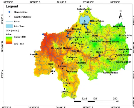
The UBNRB is located in north-western Ethiopia. Its catch-ment area is about 172 760 km2. Highlands, hills, valleys, and occasional rock peaks with elevations ranging from 500 to above 4000 m a.s.l. typically characterise the basin’s to-pography (Fig. 1). According to BCEOM (1998), two-thirds of the basin lies in Ethiopia’s highlands, with annual rain-fall ranging from 800 to 2200 mm. The central and south-eastern areas are characterised by relatively high rainfall (1400 to 2200 mm), whereas in most of the eastern and north-western parts of the basin, rainfall is less than 1200 mm. Fenta Mekonnen and Disse (2018) showed that the UBNRB has a mean areal annual rainfall of 1452 mm and mean annual minimum and maximum temperatures of 11.4 and 24.7◦C,
respectively.
Figure 1.Locations of study area and meteorological and discharge stations, with the digital elevation model (DEM) data as the background (where 1 denotes stations used for SWAT model, 2 denotes stations used for trend analysis, and 3 denotes stations removed from the analysis).
Table 1.The UBNRB’s areal long-term (1971–2010) mean annual and seasonal rainfall and streamflow.
Amount Contribution (%)
Station Kiremit Belg Bega Total Kiremit Belg Bega Mean Area (km2)
Flow (m3s−1) 3506.3 300.4 1018.4 4825.1 72.7 6.2 21.1 1608 172 254
Flow (billion m3) 36.4 3.1 10.6 50.7
Rainfall (mm) 1070.1 140.8 238.9 1449.8 73.8 9.7 16.5
Kiremit: long rainy season, Belg: short rainy season, Bega: dry season.
during this season. A dry season (Bega) lasts from October to January, and the short rainy season (Belg) lasts from Febru-ary to May. According to BCEOM (1998), the average an-nual discharge (1960 to 1992) at the Ethiopia–Sudan border (El Diem) is about 49.4 billion m3, with the low-flow month (April) equivalent to less than 2.5 % of that of the high-flow month (August). The analysis of this study revealed that the long-term (1971–2010) mean annual volume of streamflow
[image:3.612.92.500.504.579.2]wood-lands, bush, and shrubs are the dominant forms of land cover (BCEOM, 1998).
3 Input data sources
In this study, non-parametric Mann–Kendall (MK; Kendall, 1975; Mann, 1945) statistics and the SWAT, developed by the Agricultural Research Service of the United States De-partment of Agriculture (USDA-ARS; Arnold et al., 1998), are used for statistical trend analysis and water-balance mod-elling, respectively. Details of both methods are available in Sect. 4. The input data sets used for the SWAT model can be categorised into those containing weather and streamflow data and spatially distributed data sets.
3.1 Weather and streamflow data
The daily weather variables used in this study for trend analy-sis and for driving the water-balance model are precipitation, minimum air temperature (Tmin), maximum air temperature
(Tmax), relative humidity (RH), hours of sunshine (SH), and
wind speed (WS). Weather data from 40 meteorological sta-tions were obtained from the Ethiopian National Meteorolog-ical Services Agency (ENMSA) for the 1971–2010 period. Daily streamflow data for 25 gauging stations were collected from the Federal Ministry of Water, Irrigation and Electric-ity of Ethiopia for the same period 1971–2010. After screen-ings and rigorous analyses of the weather data, a considerable amount of time series data were found to be missing in most of the stations (see Table S1 in the Supplement). The occur-rences of civil war and defective and outdated devices were the main causes for the missing data records. As a result, only the 15 stations (Fig. 1) in which rainfall data are relatively more complete proved to be suitable for trend analysis. Some 10 stations having complete climate variables, such asTmax,
Tmin, RH, WS, and SH, were used as input for the SWAT
model (Fig. 1).
We resorted to spatial interpolation techniques, such as the inverse distance weighting (IDW) and linear regression (LR), to fill the gaps. Uhlenbrook et al. (2010) applied sim-ilar approaches or methods to the Gilgel Abbay sub-basin, which is the UBNRB’s headwater. The selection and num-ber of adjacent stations for interpolation are important for the accuracy of interpolated values. As mentioned by Wolde-senbet et al. (2017a), different authors used different criteria to select neighbouring stations. Because of the relatively low number of network stations, a geographic distance of 100 km was considered for most stations when selecting neighbour-ing stations. If no station was located within 100 km of the target station, then the search distance was increased until at least one suitable station is reached. After the neighbouring stations were selected, the two methods (IDW and LR) were tested by means of cross-validation to fill in missing data sets. The candidate methods’ performances were evaluated
us-ing the statistical metrics such as the root-mean-square error (RMSE), mean absolute error (MAE), correlation coefficient (R2), and percent bias (% bias) between observed and esti-mated values for the target stations. Equally weighted statis-tical metrics are applied to compare the performances of se-lected methods at target stations and to establish the ranking. A score was assigned to each candidate method according to the individual metrics. For example, the candidate achieving the smallest values of RMSE and MAE or the smallest per-centage of bias received score 1, and score 2 was assigned to the one with the larger value. The final score is obtained by summing up the score pertaining to each candidate ap-proach at each station. The method with the smallest score is the best. The monthly, seasonal, and annual weather data were aggregated from the daily time series data after filling the gaps. While filling in the missing data, uncertainty is ex-pected due to low station density, poor correlations, and the considerable number of missing records. Similar techniques and approaches were used for the analysis and filling in of missing streamflow data records.
3.2 Spatial data
Spatially distributed data required for the SWAT model in-cludes tabular and spatial soil data, tabular and spatial LULC information, and elevation data. A Shuttle Radar Topo-graphic Mission digital elevation model (SRTM DEM) with a resolution of 90 m from the Consultative Group on Interna-tional Agricultural Research – Consortium for Spatial Infor-mation (CGIAR-CSI; http://srtm.csi.cgiar.org/SELECTION/ inputCoord.asp, last access: 21 February 2015) – was used to represent land-surface drainage patterns. Terrain charac-teristics, such as slope gradient and the slope length of the terrain, and stream network characteristics, such as channel slope, length, and width, were derived from the digital eleva-tion model (DEM).
The soil map (1:5 000 000) developed by the Food and Agriculture Organization of the United Nations (FAO-UNESCO) was downloaded from http://www.fao. org/soils-portal/soil-survey/soil-maps-and-databases/ faounesco-soil-map-ofthe-world/en/, last access: 4 April 2017. Soil information, such as the soil textu-ral and physiochemical properties needed for the SWAT model, were extracted from the Harmonized World Soil Database v1.2, a database that combines existing re-gional and national soil information (http://www.fao. org/soils-portal/soil-survey/soil-maps-and-databases/ harmonized-world-soil-databasev12/en/, last access: 4 April 2017) with information provided by the FAO-UNESCO soil map (Polanco et al., 2017).
4 Methodology
4.1 Trend analysis
The non-parametric Mann-Kendall (MK; Kendall, 1975; Mann, 1945) statistic is chosen to detect trends for rainfall and streamflow time series data, as it is widely used for water resource planning, design, and management (Yue and Wang, 2004). Its advantage over parametric tests such asttest is that the MK test is more suitable for non-normally distributed and missing data, which are frequently encountered in hydrolog-ical time series (Yue et al., 2004). However, the existence of positive serial correlation in time series data affects the MK test results. If serial correlation exists in time series data, the MK test rejects the null hypothesis of no trend detection more often than specified by the significance level (Von Storch, 1995).
Von Storch (1995) proposed a prewhitening technique to limit the influence of serial correlation on the MK test. The effective or equivalent sample size (ESS) method developed by Hamed and Rao (1998) has also been proposed to mod-ify the variance. However, the study by Yue et al. (2002) re-ported that von Storch’s prewhitening is effective only when no trend exists, and the ESS approach’s rejection rate af-ter modifying the variance is much higher than the actual (Yue et al., 2004). Yue et al. (2002) then proposed trend-free prewhitening (TFPW) prior to applying the MK trend test in order to minimise its limitation. This study therefore employed TFPW to remove the serial correlation and to de-tect a trend in time data series with significant serial corre-lation. Further details can be found in (Yue et al., 2002). All the trend results in this study have been evaluated at the 5 % level of significance to ensure the effective exploration of the trend.
4.2 Change point test
The Pettitt test is used to identify whether or not there is a point change or jump in the data series (Pettitt, 1979). This method detects one unknown change point by considering a sequence of random variables(Xt)=X1, X2, . . ., XN, XN+ 1, . . ., XT that may have a change point at N, if the Xt variable for t=1,2, . . . , N time step has a common dis-tribution function, F1(x), and Xt for t=N+1, . . . ; T time step has a common distribution function,F2(x), where F1(x)6=F2(x).
4.3 Sen’s slope estimator
The trend magnitude is estimated using a non-parametric median-based slope estimator proposed by (Sen, 1968), as it is not greatly affected by gross data errors or outliers and can be computed when data are missing. The slope estimation is
given by
β=Median
X
j−Xk j−k
for all k < j, (1)
wherexj andxk are the sequential data values, andnis the number of the recorded data. 1< k < j < n, andβ is con-sidered as the median of all possible combinations of pairs for the whole data set. A positive value of β indicates an upward (increasing) trend, and a negative value indicates a downward (decreasing) trend in the time series. All MK trend tests, Pettitt change-point detections, and Sen’s slope analy-ses were conducted using the XLSTAT add-in tool from Ex-cel (https://www.xlstat.com).
4.4 Remote-sensing land-use and land-cover map 4.4.1 Landsat image acquisition
Landsat images from the years 1973, 1985, 1995, and 2010 were accessed from the US Geological Survey (USGS) Cen-ter for Earth Resources Observation and Science (EROS) via http://glovis.usgs.gov (last access: 29 December 2016). The Landsat images were selected based on the criteria of the ac-quisition period, availability, and percentage of cloud cover. Hayes and Sader (2001) recommend acquiring images from the same acquisition period to reduce the image-to-image variation caused by the sun angle, soil moisture, atmospheric condition, and vegetation-phenology differences. Cloud-free images were hence collected for the dry months of January to May. However, as the basin covers a large area, each of the LULC map’s periods comprised 16 Landsat images. Access-ing all the images durAccess-ing a dry season in a sAccess-ingle year was therefore difficult. Hence, images were acquired±1 year for each time period, and some images were also acquired in the months of November and December. For example, 16 Landsat MSS image scenes were acquired in 1973 (10 im-ages in January, four imim-ages in December and two imim-ages in November;±1 year) and were merged to arrive at one LULC representation for selected years. Please see Table S2 in the Supplement for the details on Landsat images.
4.4.2 Preprocessing and processing images
classes were then digitised using ground truth data. The sam-ples for each land cover type were then aggregated. Finally, a supervised classification was performed using a maximum likelihood algorithm to extract four LULC classes.
A total of 488 ground control points (GCPs) regarding land-cover types and their spatial locations were collected from field observations in March and April 2017 using a global positioning system (GPS). Reference data were col-lected and taken from areas where there had not been any significant land-cover change between 2017 and 2010. These areas were identified by interviewing local elderly people and were supplemented using high-resolution Google Earth im-ages and the first author’s prior knowledge. As many as 288 GCPs were used for accuracy assessment, and 200 points served as training sites to generate a signature for each land-cover type. The classifications’ accuracy was assessed by computing the error matrix (also known as the confusion ma-trix), which compares the classification result with ground truth information as suggested by DeFries and Chan (2000). A confusion matrix lists the values for the reference data’s known cover types in the columns and for the classified data in the rows (Banko, 1998), as shown in Table 5. From the confusion matrix, statistical metrics of overall accuracy, pro-ducers’ accuracy, and users’ accuracy are used. Another dis-crete multivariate technique useful in accuracy assessment is called KAPPA (Congalton, 1991). The statistical metric for KAPPA analysis is the Kappa coefficient, which is an-other measure of the proportion of agreement or accuracy. The Kappa coefficient is computed as
K=
N i=r P i=1
xii r P i=1
(xi+×x+i)
N2−Pr i=1
(xi+×x+i)
, (2)
whereris the number of rows in the matrix,xiiis the number of observations in rowiand columni, andxi+andx+i are the marginal totals of rowiand columni, respectively.N is the total number of observations.
Once the land-cover classification of the year 2010 Land-sat image had been completed and its accuracy checked, the normalised difference vegetation index (NDVI) differencing technique (Mancino et al., 2014) was applied to classify the images from 1973, 1985, and 1995. This technique was cho-sen to increase the accuracy of classification, as it is hard to find an accurately classified digital or analog LULC map of the study area during 1973, 1985, and 1995. The informa-tion obtained from the elders is also more subjective, and its reliability is questionable when there is a considerable time gap. We first calculated the NDVI from the Landsat MSS (1973) and three preprocessed Landsat TM images (1985, 1995, and 2010), following the general normalised differ-ence between band TM4 and band TM3 images (Eq. 3). The resulting successive NDVI images were subtracted from each other to assess the1NDVI image with positive
(vegeta-tion increase), negative (vegeta(vegeta-tion cleared), and no changes at a 30 m×30 m pixel resolution (Eqs. 4–6). The Landsat MSS 60 m×60 m pixel-size data sets were resampled to a 30 m×30 m pixel size using the “nearest neighbour” tech-nique to have equal pixel sizes for the different images with-out altering the image data’s original pixel values. This pro-cess is represented by the following:
NDVI=(TM4−TM3)
(TM4+TM3) or
(MSS3−MSS2)
(MSS3+MSS2)
, (3)
1NDVI1995/2010=NDVI1995−NDVI2010, (4)
1NDVI1985/1995=NDVI1985−NDVI1995, (5)
1NDVI1973/1985=NDVI1973−NDVI1985. (6)
The1NDVI image was then reclassified using a threshold value calculated asµ±nσ; whereµrepresents the1NDVI pixels value mean, andσ represents the standard deviation. The threshold identifies three ranges in the normal distribu-tion: (a) the left tail (1NDVI< µ−nσ), (b) the right tail (1NDVI> µ+nσ), and (c) the central region of the nor-mal distribution (µ−nσ < 1NDVI< µ+nσ). Pixels within the two tails of the distribution are characterised by signif-icant land-cover changes, whereas pixels in the central re-gion represent no change. To be more conservative,n=1 was selected for this study in order to narrow the threshold ranges for reliable classification. The standard deviation (σ ) is one of the most widely applied threshold identification ap-proaches for different natural environments based on differ-ent remotely sensed imagery (Hu et al., 2004; Jensen, 1996; Lu et al., 2004; Mancino et al., 2014; Singh, 1989), as cited by Mancino et al. (2014).
4.5 SWAT hydrological model
The SWAT is an open-source-code, semi-distributed model with a large and growing number of model applications in a variety of studies, ranging from catchment to continental scales (Allen et al., 1998, 2012; Neitsch et al., 2002). It en-ables the impact of LULC change and climate change on water resources to be evaluated in a basin with varying soil, land-use, and management practices over a set period of time (Arnold et al., 2012).
In SWAT, the watershed is divided into multiple sub-basins, which are further subdivided into hydrological re-sponse units (HRUs) consisting of homogeneous land-use management, slope, and soil characteristics (Arnold et al., 1998; Arnold et al., 2012). HRUs are the smallest units of the watershed in which relevant hydrologic components, such as evapotranspiration, surface runoff and peak rate of runoff, groundwater flow, and sediment yield, can be estimated. Wa-ter balance is the driving force behind all of the processes in the SWAT calculated using Eq. (7),
SWt=SWo+
t X i=1
(7) Rday−Qs−Ql−Qb−Ea−Revap−DA_recharge,
where SWt is the final soil-water content (mm H2O), SWo
is the initial soil-water content on day i (mm H2O), t is
the time (days),Rday is the amount of precipitation on day
i (mm H2O), Qs is the amount of surface runoff on day
i (mm H2O), Ql is the amount of return flow on day i
(mm H2O),Qb is the return flow from the shallow aquifer
on dayi(mm H2O),Eais the amount of evapotranspiration
from the canopy and soil surface on dayi(mm H2O), Revap
is the amount of water transferred from the underlying shal-low aquifer reversely upward to the soil-moisture storage on dayi(mm H2O) in response to water demand for
evapotran-spiration, and DA_recharge is the amount of water recharge to the deep aquifer on dayi(mm H2O).
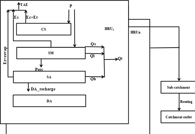
Runoff is calculated separately for each HRU and routed to obtain the total streamflow for the watershed using either the soil-conservation-service (SCS) curve-number (CN) method (Mockus, 1964) or the Green–Ampt infiltration method (GAIM; Green and Ampt, 1911; see Fig. 2). However, spa-tial connectivity and interactions among HRUs are ignored. Instead, the cumulative output of each spatially discontinu-ous HRU at the sub-watershed outlet is directly routed to the channel (Pignotti et al., 2017). This lack of spatial connec-tivity among HRUs makes implementation and the impact analysis of spatially targeted management such as the soil-and-water conservation structure difficult to incorporate into the model. Different authors have made efforts to overcome this problem, for instance, a grid-based version of the SWAT model (Rathjens et al., 2015) or a landscape simulation on a regularised grid (Rathjens and Oppelt, 2012). Moreover, Arnold et al. (2010) and Bosch et al. (2010) further
mod-ified SWAT so that it allows landscapes to be subdivided into catenas comprising upland, hillslope, floodplain units, and flow to be routed through these catenas. However, the SWAT grid, developed to overcome this limitation, remains largely untested and computationally demanding (Rathjens et al., 2015).
Hence, the standard SWAT CN method was chosen for this study, because it was applied in many Ethiopian watersheds (Gashaw et al., 2018; Gebremicael et al., 2013; Setegn et al., 2008; Woldesenbet et al., 2017b). Furthermore, its ability to use daily input data (Arnold et al., 1998; Neitsch et al., 2011; Setegn et al., 2008) as compared to the GAIM, which re-quires subdaily precipitation as a model input that can be dif-ficult to obtain in data-scarce regions like the UBNRB. This study focused on the effects of LULC change and climate change on the basin’s water-balance components, which in-clude the components of inflows, outflows, evapotranspira-tion, losses, and the change in storage as shown in the general water balance in Eq. (8).
R=Qt+TAE+Losses+1S, (8)
whereQt=Qs+Ql+Qband total actual evapotranspiration
TAE=Ec+Es+Et+Er, as shown in Fig. 2.
Ris the amount of precipitation (mm d−1) as the main in-flow,Qtis the total amount of streamflow (mm d−1) as
out-flow, TAE is the total actual evapotranspiration (mm d−1), Ec is evaporation from the canopy surface (mm d−1),Et is
the amount of plant transpiration (mm d−1),Es is
evapora-tion from the soil surface (mm d−1),Er or Revap is
evap-oration from the shallow aquifer (mm d−1; Abiodun et al., 2018), losses are the amount of water lost from the system as a recharge to the deep aquifer (DA_recharge; mm d−1), and
1Sis the change in soil-water storage (mm d−1). SWAT has
four storages: canopy storage (CS), soil moisture (SM), shal-low aquifer (SA), and deep aquifer (DA). Water movement from the soil-moisture storage to the shallow aquifer is due to percolation, whereas water movement from the shallow aquifer reversely upward to the soil-moisture storage is Re-vap, and further water movement from the shallow aquifer to the deep aquifer is recharge. For a more detailed description of the SWAT model, refer to Neitsch et al. (2011).
HRUn
Sub-catchmentt
Catchment outlett
Routing HRU1
P
Ec+Et
DA SM
SA CS
DA_recharge
E
r=
re
va
p
Perc
Qs
Ql
Qb
Qt Es
[image:8.612.137.465.74.300.2]TAE
Figure 2.Schematic representation of the SWAT model structure modified from Marhaento et al. (2017).P is precipitation; CS is canopy storage; TAE is total actual evapotranspiration;Ecis evaporation from the canopy surface;Es is evaporation from the soil surface;Etis transpiration from plants; Perc is percolation from the soil storage to shallow aquifer; SM is soil-moisture storage; SA is shallow aquifer; Er=Revap is evaporation from the shallow aquifer;Qtis total streamflow; DA is deep aquifer; HRU is hydrological response unit;Qbis base flow;Qlis lateral flow; andQsis surface runoff.
model’s input parameters to match model output with ob-served data, thereby reducing the prediction uncertainty. Ini-tial parameter estimates were taken from the default lower and upper bound values of the SWAT model database and from earlier studies in the basin, such as that of Gebremi-cael et al. (2013). The final step, model validation, involves running a model using parameters that were determined dur-ing the calibration process and compardur-ing the predictions to independently observed data not used in the calibration.
In this study, both manual and automatic calibration strate-gies were applied to attain the minimum differences between observed and simulated streamflows in terms of surface flow, peak flow, and total flow, following the steps recommended by Arnold et al. (2012). For the purpose of impact analy-sis, we divided the simulation period 1971–2010 into four decadal periods, hereafter referred as the 1970s (1971–1980), 1980s (1981–1990), 1990s (1991–2000), and 2000s (2001– 2010), as shown in Table 2. The model’s performance for the streamflow was then evaluated using statistical methods (Moriasi et al., 2007) such as the Nash–Sutcliffe coefficient of efficiency (NSE), the coefficient of determination (R2), and the relative volume error (RVE %), which are shown in Eq. (9)–(11). Furthermore, graphical comparisons of the sim-ulated and observed data, as well as water-balance checks, were used to evaluate the model’s performance. This
evalua-tion may be represented by the following:
R2=
n
P I=1
Qm,i−Qm
Qs,i−Qs
2
n P I=1
Qm,i−Qm
2Pn I=1
(Qs,i−Qs)2
, (9)
NSE=1−
n P I=1
Qm,−Qs
2
i
n P I=1
Qm,i−Qm
2
, (10)
RVE(%)=100×
n P i=1
(Qm−Qs)i n
P i=1
Qm,i
, (11)
whereQm,i is the measured streamflow in m3s−1,Qm are
the mean values of the measured streamflow (m3s−1),Qs,i is the simulated streamflow in m3s−1, andQsare the mean
values of simulated data in m3s−1. 4.6 SWAT simulations
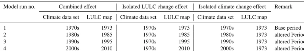
Table 2.Data sets of the baseline and altered periods for the SWAT simulation used to analyse the combined and isolated effect of LULC and climate change on streamflow and water-balance components.
Model run no. Combined effect Isolated LULC change effect Isolated climate change effect Remark
Climate data set LULC map Climate data set LULC map Climate data set LULC map
1 1970s 1973 1970s 1973 1970s 1973 Base period
2 1980s 1985 1970s 1985 1980s 1973 altered Period 1
3 1990s 1995 1970s 1995 1990s 1973 altered Period 2
4 2000s 2010 1970s 2010 2000s 1973 altered Period 3
LULC change and climate change. We followed the ap-proach in Marhaento et al. (2017) and divided the analy-sis period, 1971–2010, into four periods of similar length (four decades). These are periods when land-use changes are expected to change the hydrological regime within a catchment (Marhaento et al., 2017; Yin et al., 2017). The first period, the 1970s, was regarded as the baseline period. The other periods, the 1980s, 1990s, and 2000s, were re-garded as altered periods. LULC maps of 1973, 1985, 1995, and 2010 were used to represent LULC patterns during the 1970s, 1980s, 1990s, and 2000s, respectively. For analyses, the SWAT model was calibrated and validated for each re-spective period using the rere-spective LULC map and weather data (Table 2). The DEM and soil data sets remained un-changed. The differences between the simulation result of the baseline and altered periods represent the combined ef-fects of LULC and climate change on streamflow and water-balance components.
The second approach included simulations that attribute the effects from LULC changes alone. It aimed to investi-gate whether LULC change is the main driver for changes in water-balance components. To identify the hydrological im-pacts caused solely by LULC, a “fixing–changing” method was used (Marhaento et al., 2017; Woldesenbet et al., 2017b; Yan et al., 2013; Yin et al., 2017). The calibrated and vali-dated SWAT model and its parameter settings in the baseline period were forced by weather data from the baseline pe-riod, 1973–1980, while changing only the LULC maps from 1985, 1995, and 2010, keeping the DEM and soil data con-stant (Hassaballah et al., 2017; Marhaento et al., 2017; Wold-esenbet et al., 2017b; Yin et al., 2017). We ran the calibrated SWAT model for the baseline period (1970s) four times, only changing the LULC map for the years 1973, 1985, 1995, and 2010 and retaining the constant weather data set from the 1970s (Table 2). The third approach is similar to the second, but the simulations are attributed only for climate change. The calibrated models for the baseline period were run again four times, corresponding to the LULC periods us-ing a unique LULC map of the year 1973 but alterus-ing the four different periods of weather data sets for their respective periods.
5 Results and discussions 5.1 Trend test
5.1.1 Rainfall
Table 3.MK and Pettitt tests for the UBNRB’s rainfall and streamflow after TFPW at different timescales.
Streamflow Rainfall
pvalue pvalue
Time After∗ Before∗ Sen’s Change Pettitt After∗ Before∗ Sen’s Change Pettitt
scale slope point test slope point test
Daily <0.0001 <0.0001 0.013 1987 Increasing 0.387 0.953 0.000 1988 Increasing
Monthly <0.0001 0.031 0.378 No change 0.010 0.640 0.009 No change
Annually <0.0001 0.009 9.619 1995 Increasing 0.006 0.260 1.886 No change
Kiremit <0.0001 0.014 20.30 No change 0.010 0.348 1.364 No change
Belg <0.0001 0.004 3.593 1985 Increasing 0.822 0.935 0.068 No change
Bega 0.000 0.214 4.832 No change 0.527 0.755 0.169 No change
∗Before and after TFPW;pprobability at 5 % significance level.
1200 1300 1400 1500 1600 1700
1970 1980 1990 2000 2010 2020
Pr
ec
ipi
ta
tion
(m
m
)
Year
Areal rainfall
mu = 1450
1000 1200 1400 1600 1800 2000 2200 2400
1970 1980 1990 2000 2010 2020
St
re
am
flow
(m
3s -1)
Year
Streamflow
mu1 = 1510 mu2 = 1784
y = 1.8344x + 1412.2 R² = 0.0403
1200 1300 1400 1500 1600 1700 1800
1971 1976 1981 1986 1991 1996 2001 2006
R
ai
nf
al
l (
m
m
)
Year
Areal rainfall
y = 10.474x + 1399.1 R² = 0.2226
800 1000 1200 1400 1600 1800 2000 2200 2400
1971 1976 1981 1986 1991 1996 2001 2006
S
tr
ea
m
fl
ow
(m
3s -1)
Year
Streamflow
(b) (a)
(d) (c)
Figure 3.The Pettitt homogeneity test’s(a)annual rainfall,(b)annual flow of the UBNRB,(c)linear trend of mean annual rainfall, and
(d)linear trend of mean annual streamflow, where mu is the mean annual precipitation (mm), mu1 is the mean annual precipitation before change (mm), and mu2 is the mean annual precipitation after change (mm).
series from station data. A summary is provided in Table 3 and Fig. 3. The MK test showed increasing trends for an-nual, monthly, and long rainy-season rainfall series, whereas no trend for daily, short rainy, and dry season rainfall series appeared. The magnitude of trends for annual, monthly, and long rainy-season rainfall series are not statistically signif-icant, as explained by the values of Sen’s slope. However, the Pettitt test could not detect any jump point in basin-wide rainfall series except for daily time series rainfall (see Fig. S1 in the Supplement).
[image:10.612.104.487.254.530.2]Network (GHCN) database and 10 day rainfall data for the 10 selected stations obtained from the National Meteorolog-ical Service Agency of Ethiopia from 1963 to 2003. Con-way (2000) also constructed basin-wide annual rainfall in the UBNRB for the 1900–1998 period from the mean of 11 gauges. Furthermore, (Conway, 2000) employed simple linear regressions over time to detect trends in annual rain-fall series without removing the serial autocorrelation effects. Gebremicael et al. (2013), used only nine stations from the 1970–2005 period. However, in this study, we used daily ob-served rainfall data from 15 stations collected from Ethiopian Meteorological Agency from 1971 to 2010. The stations are more or less evenly distributed over the UBNRB.
5.1.2 Streamflow
The MK test’s result for daily, monthly, annual, and seasonal (long and short rainy season and dry season) streamflow time series showed a positive trend, the magnitude of which is sta-tistically significant, as summarised in Table 3. The Pettitt test also detected change points for daily, annual, and short rainy-season streamflow but did not detect change points for monthly, long, and dry season streamflow (see Figs. 3 and S2). The change point detected by the Pettitt test for annual streamflow is in 1995, whereas for daily and short rainy sea-sons, it is in 1985 and 1987, respectively. The result obtained from the MK test agrees well with the findings in Gebremi-cael et al. (2013), who reported an increasing trend in the ob-served annual, short, and long rain seasons’ streamflow at the El Diem gauging station, but our results disagree with find-ings for dry-season streamflow. Furthermore, the increasing trend of long rainy-season streamflow agrees well with the result of Tesemma et al. (2010), but it disagrees with the re-sults of short rainy season and annual flows. Tesemma et al. (2010) reported that the short rainy season and the annual flows are constant for the 1964–2003 period. This disagree-ment is likely attributable to the difference in analysis period, as can be seen from Fig. 3. The last 7 years, 2004–2010, had relatively higher streamflow records.
Although, the results of the MK test for annual and long rainy-season rainfall and streamflow show an increasing trend for the last 40 years in the UBNRB, the magnitude of Sen’s slope for streamflow is much greater than it is for rainfall (Table 3). Moreover, short rainy-season streamflow shows a statistically significant positive increase, whereas the rainfall shows no change. The mismatch between the rain-fall and the streamflow trend magnitude could be associated with evapotranspiration and could be attributable to the com-bined effect of LULC change, climate change, the infiltration rate due to changing soil properties, rainfall intensity, and ex-treme events.
5.2 LULC change analysis
According to the confusion-matrix report, with an overall ac-curacy of 80 %, a producer’s acac-curacy values for all classes ranged from 75.4 % to 100 %, user’s accuracy values ranged from 83.7 % to 91.7 %, and a kappa coefficient (k) of 0.77 was attained for the 2010 classified image (Table 5). Mon-serud (1990) suggested a kappa value of <40 % as poor, 40 %–55 % as fair, 55 %–70 % as good, 70 %–85 % as very good, and>85 % as excellent. According to these ranges, the classification in this study has very good agreement with the validation data set and meets the minimum accuracy re-quirements to be used for further change detection and im-pact analysis.
The classified images of the basin (Fig. 4) have shown different LULC proportions at four distinct time periods, as shown in Fig. 5. In 1973, cultivated land dominantly cov-ered (62.9 %) the UBNRB, followed by bushes and shrubs (18 %), forest (17.4 %), and water (1.74 %). In 1985, culti-vated land area increased to 65.6 %, followed by bushes and shrubs (18.3 %), while forest decreased to 14.4 %, and wa-ter remained unchanged at 1.7 %. In 1995, cultivated land area further increased to 67.5 %, followed by bushes and shrubs (18.5 %). Forest further decreased to 12.2 %, and wa-ter remained unchanged at 1.7 %. In 2010, cultivated land decreased to 63.9 %, bushes and shrubs increased to 18.8 %, forest increased to 15.6 %, and water remained unchanged at 1.7 %. During the entire 1973–2010 period, cultivated land, along with bushes and shrubs, remained the major propor-tions compared to the other LULC classes. The highest in-crease (2.7 %) and the largest dein-crease (−3.6 %) in cultivated land occurred during the 1973–1985 and 1995–2010 peri-ods, respectively. The largest increase in bushes and shrubs was 0.3 % from 1973 to 1985, whereas the largest increase in forest coverage (3.4 %) was recorded during the 1995–2010 period. Water coverage remained unchanged from 1973 to 2010.
land-Table 4.Confusion (error) matrix for the 2010 land-use and land-cover classification map.
LULC class Water Forest Cultivated Bushes Row Producers
and shrubs total accuracy
Water 44 0 0 0 44 100
Forest 1 46 6 8 61 75.4
Cultivated land 2 3 77 15 97 79.4
Bushes and shrubs 1 3 9 73 86 84.9
Column total 48 52 92 86 288
Users’ accuracy (%) 91.7 88.5 83.7 84.9
Overall accuracy (%) 80
Kappa 0.77
cover mapping is reasonably accurate overall, providing a good base for land-cover estimation and for providing basic information for the hydrological impact analysis.
The rate of expansion of cultivated land before 1995 was higher than after 1995. Conversely, the area of the forest land decreased in 1985 and 1995 with reference to the 1973 base-line. However, after 1995, the forest’s size increased again, whereas cultivated land decreased. The increased forest cov-erage and the decrease in cultivated land over the period 1995 to 2010 showed that the environment was recovering from the devastating drought, and forest clearing for firewood and cultivation due to population growth has been minimised. This could be due to the afforestation programme, which the Ethiopian government initiated, and to the extensive soil-and-water conservation measures carried out by the commu-nity. Since 1995, eucalyptus tree plantations expanded sig-nificantly across the country at the homestead level for fire-wood, construction materials, charcoal production, and in-come generation (Woldesenbet et al., 2017b). In summary, forest coverage decreased by 1.8 %, while both bushes and shrubs as well as cultivated land increased by 0.8 % and 1 %, respectively, from the original 1973 level to the 2010 period. This result agrees well with other studies (Gebremicael et al., 2013; Rientjes et al., 2011; Teferi et al., 2013; Woldesenbet et al., 2017b), which reported a significant conversion of nat-ural vegetation cover into agricultnat-ural land.
5.3 SWAT model calibration and validation
[image:12.612.130.467.86.208.2]The SWAT model’s most sensitive parameters for simulating streamflow were identified using a global sensitivity analy-sis of SWAT-CUP. Their optimised values were determined by the calibration process that Arnold et al. (2012) recom-mended. Parameters such as the SCS curve number (CN2), base-flow alpha factor (ALPHA_BF), soil evaporation com-pensation factor (ESCO), threshold water depth in the shal-low aquifer required for return fshal-low to occur (GWQMN), groundwater “Revap” coefficient (GW_REVAP), and avail-able water capacity (SOL_AWC) were found to be the most sensitive parameters for the streamflow predictions.
Table 5.The SWAT model’s statistical performance measure val-ues.
Period R2 NSE RVE (%)
1970s Calibration (1973–1977) 0.79 0.74 −3.41
Validation (1978–1980) 0.84 0.83 7.18
1980s Calibration (1983–1987) 0.80 0.74 −0.72
Validation (1988–1990) 0.86 0.82 0.73
1990s Calibration (1993–1997) 0.91 0.91 1.79
Validation (1998–2000) 0.87 0.84 −3.56
2000s Calibration (2003–2007) 0.86 0.86 3.99
Validation (2008–2010) 0.94 0.92 −7.51
[image:12.612.308.547.260.404.2]Figure 4.Land-cover map of UBNRB derived from Landsat images from(a)1973,(b)1985,(c)1995, and(d)2010a(b).
5.4 Combined effects of LULC change and climate change on streamflow and water-balance components
The simulation results of the four independent, decadal-time-scale calibrated and validated SWAT model runs reflect the combined effect of both LULC and climate change during the past 40 years (Table 8). From the simulation result, mean annual streamflow increased by 16.9 % between the 1970s and the 2000s, while the observed mean annual streamflow increased by 15.3 % for the same period. However, the rate of change is different in different decades. For example, it
increased by 3.4 % and 9.9 % during the 1980s and 1990s, respectively, from the baseline 1970s period.
The ratio of mean annual streamflow to mean annual pre-cipitation (Qt/P) increased from 19.4 % to 22.1 %, while the
actual evaporation to precipitation (Ea/P) ratio decreased
from 61.1 % to 60.5 % from the 1970s to 2000s. Moreover, the ratio of surface runoff to streamflow (Qs/Qt) increased
notably, from 40.7 % in the 1970s to 50.1 % and 55.4 % in the 1980s and 1990s, respectively, and it decreased to 43.7 % in the 2000s. In contrast, the base-flow-to-streamflow ra-tio (Qb/Qt) notably decreased from 17.1 % in the 1970s to
(a) (b)
17.4 14.4 12.2 15.6
18.0 18.3 18.5 18.8
62.9 65.6 67.5 63.9
0 20 40 60 80 100 120
1973 1985 1995 2010
A
re
a
c
ove
ra
ge
(
%
)
Water Forest Bushes and shrub Cultivated
-17.3 -14.9
27.7
1.8 1.4
1.2
4.3 2.9
-5.3
-20 -10 0 10 20 30 40
1973–1985 1985–1995 1995–2010
L
and
c
ove
r c
ha
nge
(
%
)
Water Forest Bushes and shrub Cultivated
[image:14.612.88.504.63.204.2]Figure 5. (a)LULC composition and(b)LULC change in the UBNRB during the period from 1973 to 2010.
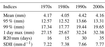
Table 6.Summary of the UBNRB’s precipitation indices at decadal time series.
Indices 1970s 1980s 1990s 2000s
Mean (mm) 4.17 4.05 4.42 4.16
95 % (mm) 12.57 12.52 13.66 13.31
99 % (mm) 17.34 17.77 19.44 19.65
1 day max (mm) 27.15 25.67 32.24 32.38
R20 mm (days) 16 15 30 35
SDII (mm d−1) 7.22 7.38 7.66 7.77
SDII is the ratio of total precipitation (mm) to R1 mm (days).
but it increased to 20 % in the 2000s. The result for surface runoff agrees with findings in Gebremicael et al. (2013), but disagreement is observed for base flow. The study reported that the surface runoff (Qs) contribution to the total river
discharge increased by 75 %, while the base flow (Qb)
de-creased by 50 % from the 1970s to 2000s.
In general, 1.8 % forest cover loss and 1 % increased cul-tivated land combined with 2.2 % increased rainfall from the 1970s to the 2000s led to a 16.9 % increase in simu-lated streamflow. The 1990s was the period during which the greatest deforestation and expansion of cultivated land was reported; meanwhile, it was the time when the rainfall intensity and the number of rainfall events significantly in-creased compared to the 1970s and 1980s, as shown in Ta-ble 4. Hence, the increased mean annual streamflow could be ascribed to the combined effects of LULC and climate change. In the case of (Qs/Qt), the increasing pattern could
be ascribed to increasing rainfall intensities, the expansion of cultivated land, and the diminution of forest coverage, which might adversely affect soil and water storage and decrease rainfall infiltration, thereby increasing water yield or stream-flow. In contrast, the decreasingQb/Qtis positively related
to the increasing evapotranspiration linked to both LULC and climate factors (Table 8). This hypothesis can be explained with the change in CN2 parameter values obtained during calibration of the four SWAT model runs. The CN2
param-Table 7.SWAT sensitive model parameters and their (final) cali-brated values for the four model runs.
Parameter Optimum value
1970s 1980s 1990s 2000s
R-CN2 0.88 0.91 0.92 0.9
a-Alpha-BF 0.028 0.028 0.028 0.028
V-GW_REVAPMN 0.7 0.45 0.7 0.34
V-GWQMN 750 750 750 750
V-REVAPMN 550 450 425 550
a-ESCO −0.85 −0.85 −0.85 −0.85
R-SOL_AWC 6.5 6.5 6.5 6.5
Rvalue from the SWAT database is multiplied by a given value;Vreplace the initial parameter by the given value;aadding the given value to initial parameter value.
eter value, which is a function of evapotranspiration derived from LULC, soil type, and slope, increased in the 1980s and 1990s, relative to the 1970s, and could be associated with the expansion of cultivated land and shrinkage of forest land. The increasing CN2 results reflect more surface runoff and less base flow being generated.
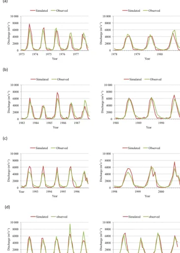
[image:14.612.65.269.277.369.2] [image:14.612.316.541.278.395.2](a) (b) (c) (d) 0 2000 4000 6000 8000 10 000
1973 1974 1975 1976 1977
D is cha rge ( m 3s -1) Year Simulated Observed 0 2000 4000 6000 8000 10 000
1978 1979 1980
D is cha rge ( m 3s -1) Year Simulated Observed 0 2000 4000 6000 8000 10 000
1983 1984 1985 1986 1987
D is cha rge ( m 3s -1) Year Simulated Observed 0 2000 4000 6000 8000 10 000
1988 1989 1990
D is cha rge ( m 3s -1) Year Simulated Observed 0 2000 4000 6000 8000 10 000
Year 1993 1994 1995 1996
D is cha rge ( m 3s -1) Year Simulated Observed 0 2000 4000 6000 8000 10 000
1998 1999 2000
D is cha rge ( m 3s -1) Year Simulated Observed 0 2000 4000 6000 8000 10 000
2003 2004 2005 2006 2007
D is cha rge ( m 3s -1) Year Simulated observed 0 2000 4000 6000 8000 10 000
2008 2009 2010 2011
[image:15.612.117.483.74.587.2]D is cha rge ( m 3s -1) Year Simulated observed
Figure 6.Calibration and validation of the SWAT hydrological model (left and right, respectively) at monthly timescale:
(a)1970s,(b)1980s,(c)1990s, and(d)2000s.
5.5 Effects of an isolated LULC change on streamflow and water-balance components
Yan et al. (2013) used a fixing–changing method, which was also applied in this study to identify the hydrological
sug-Table 8.Mean annual water-balance-component analysis in the upper Blue Nile River basin, considering LULC and climate change over their respective periods. All streamflow estimates are for the El Diem station, where water yield (Qt)=Qs+Ql+Qband change in soil storage=P−Qs−Ql−Qb−Ea-Revap-Recharge.
Unit 1970s 1980s 1990s 2000s
Precipitation (P) mm 1428.1 1397.1 1522.2 1462.5
Surface flow (Qs) mm 112.8 143.4 168.6 141.4
Lateral flow (Ql) mm 116.8 113.4 125.9 117.6
Base flow (Qb) mm 47.3 29.6 9.8 64.7
Total water yield (Qt) mm 276.9 286.3 304.3 323.7
Er=Revap (from shallow aquifer) mm 269.2 257.2 310.6 241.0
Ea(Ec+Et+Es) mm 871.6 852.6 904.3 885.0
TAE mm 1140.8 1109.8 1214.9 1126.0
Recharge (to deep aquifer) mm 16.7 15.0 16.7 16.3
Change in soil-water content mm −6.3 −14.0 −13.7 −3.5
Qs/Qt % 40.7 50.1 55.4 43.7
Qb/Qt % 17.1 10.3 3.2 20.0
Qt/P % 19.4 20.5 20.0 22.1
Er(Revap)/TAE % 23.6 23.2 25.6 21.4
Ea/P % 61.0 61.0 59.4 60.5
0.0 10.0 20.0 30.0 40.0 50.0 60.0 70.0
1973
LULCLULC1985 LULC1995 LULC2010 1970s CL 1980s CL 1990s CL 2000s CL
Effect of LULC change Effect of climate change
R
at
io
(%
)
[image:16.612.142.452.106.297.2]Qs/Qt(%) Qb/Qt(%) Qt/P(%) Ea/P(%) Revap/TAE(%)
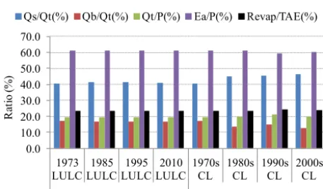
Figure 7.Ratio of water-balance component analysis at the El Diem station using an isolated effect (LULC/climate change).
gested by Hassaballah et al. (2017). The results from Fig. 7 indicated thatQs/Qt ratio changed from 40.7 % to 41.2 %,
41.9 %, and 40.9 % by using the LULC maps from 1973, 1985, 1995, and 2010, respectively, whereas theQb/Qt
ra-tio changed from 17.1 % to 16.8 %, 16.5 %, and 16.9 %, re-spectively. The largestQs/Qtratio (41.9 %) and the smallest
Qb/Qt ratio (16.5 %) were recorded with the 1995 LULC
map. This could be attributed to the 5.1 % reduction in forest coverage and the 4.6 % increase in cultivated land with the 1995 LULC map, relative to the 1973 LULC map.
On a basin scale over a decadal time period, water gains are mainly from precipitation. The losses are mainly due to runoff and evapotranspiration (Oki et al., 2006), as the losses due to the deep percolation over the whole UBNRB are neg-ligible (Steenhuis et al., 2009). The long-term mean annual deep percolation simulated in this study is about 16.7 mm
and is constant in four decadal periods, which is about 6 % of the total water yield. With the fixing–changing approach, the change in streamflow attributable to LULC change was essentially the change in evapotranspiration between the two periods, as the amount of precipitation was constant (1970s), and the change in water storage during the two periods was similar (Yan et al., 2013). AnnualEa losses from seasonal
crops are smaller than those from forests, because seasonal crops transpire during a relatively shorter time interval than perennial trees do (Yan et al., 2013). As a result, the ac-tual mean annual Ea simulated by the SWAT model was
871.6 mm at the baseline. It decreased to 871.4 and 871 mm in 1985 and 1995, respectively, and increased to 872.1 mm in 2010. This could be due to the simultaneous expansion of cultivated land and the shrinkage in forest coverage in the 1985 and 1995 LULC maps, relative to the 1973 baseline. Furthermore, this deforestation may reduce the canopy’s in-terception of the rainfall, decrease soil infiltration by increas-ing raindrop impacts, and reducincreas-ing plant transpiration, which can significantly increase surface runoff, reducing base flow (Huang et al., 2013). Here, the evapotranspiration change caused by the LULC change is minimal. As a result, the change for surface runoff and base flow is not significant. 5.6 Effects of isolated climate change on streamflow
and water-balance components
The impacts of climate change are analysed by running the four models using a unique LULC map from 1973 with its model parameters, while changing only the weather data sets from the 1970s, 1980s, 1990s, and 2000s. The simulated water-balance components shown in Fig. 7 indicate that the Qs/Qt ratio increased from 40.7 % to 45.2 %, 45.6 %, and
[image:16.612.53.282.327.461.2]respec-tively, while theQb/Qtratio changed from 17.1 % to 13.5 %,
14.9 %, and 12.7 % for the same simulation periods. The de-creasing Qb/Qt ratio for the altered periods, compared to
the baseline period, could be attributed to evapotranspira-tion changing from 872 to 854 mm, 906 mm, and 884 mm in 1970s, 1980s, 1990s, and 2000s, respectively, which can be linked to temperature and amount of rainfall. However, it is important to know the dominant rainfall–runoff process in the study area to fully understand the effect of climate change on the water-balance components.
Although no detailed research has been conducted on the upper Blue Nile River basin to investigate the runoff-generation processes, Liu et al. (2008) investigated the rainfall–runoff processes at three small watersheds located inside and around the upper Blue Nile River basin, namely Mayber, Andit Tid, and Anjeni. Their analysis showed that, unlike in temperate watersheds, in monsoonal climates, a given rainfall volume at the onset of the monsoon produces a different runoff volume than the same rainfall at the end of the monsoon. Liu et al. (2008) and Steenhuis et al. (2009) showed that the ratio of discharge to precipitation minus evapotranspiration, Q/(P–ET), increases with cumulative precipitation from the onset of a monsoon. This suggests that saturation excess processes play an important role in water-shed response.
Furthermore, the infiltration rates that Engda (2009) mea-sured in 2008 were compared with rainfall intensities in the Maybar and Andit Tid watersheds located inside and around the UBNRB. In the Andit Tid watershed, which has an area of less than 500 ha, the measured infiltration rates at 10 lo-cations were compared with rainfall intensities considered from the 1986–2004 period. The analysis showed that only 7.8 % of rainfall intensities were found to be higher than the lowest soil infiltration rate of 25 mm h−1. Derib (2005) per-formed a similar analysis in the Maybar watershed (with a catchment area of 113 ha). The infiltration rates measured from 16 measurements ranged from 19 to 600 mm h−1, with a 240 mm h−1 average and 180 mm h−1 median, whereas the average daily rainfall intensity from 1996 to 2004 was 8.5 mm h−1. Hence, he suggested from these infiltration mea-surements that infiltration excess runoff is not a common fea-ture in these watersheds.
From the above discussion points, it is to be noted that surface runoff could increase with increasing total rainfall amount, regardless of rainfall intensity. However, the mean annual rainfall amount in this study decreased from the 1970s to the 1980s (1428 and 1397 mm, respectively), while the (Qs/Qt) ratio increased from 40.7 % to 45.2 %. Similarly,
the mean annual rainfall amount in the 1990s (1522 mm) was greater than the mean annual rainfall amount in the 2000s (1462 mm) while the (Qs/Qt) increased from 45.6 %
to 46.2 %. In contrast, in climate indices such as 99 % rain-fall and SDII (ratio of total precipitation amount to num-ber of days when rainfall >1 mm; R1 mm), the number of days when rainfall>20 mm (R20 mm) increases
consis-tently from 1970 to the 2000s, as shown in Table 4. This in-dicates that the increasing surface runoff might be due to an increasing of number of extreme rainfall events and rainfall intensity. Although we did not use hourly rainfall data for the SWAT model, this study suggested that the excess infil-tration of overland flow dominates the rainfall–runoff pro-cesses in the UBNRB, not the saturation excess of overland flow. The contradiction from the previous studies might be due either to the limitation of the SWAT CN method when applied in monsoonal climates or the overlooked tillage ac-tivities, which significantly impact the soil infiltration rate. Extensive tillage activities are carried out across the basin at the beginning of the rainy season. Soils get disturbed as a result, which can increase the infiltration rate and ultimately decrease the amount of rainfall converted to runoff.
Although the CN method is easy to use and provides ac-ceptable results for discharge at the watershed outlet in many cases, researchers have concerns about its use in watershed models (Steenhuis et al., 1995; White et al., 2011). The SWAT CN model relies on a statistical relationship between soil-moisture condition and CN values obtained from plot data in the United States, with a temperate climate that was never tested in a monsoonal climate, exhibiting two extreme soil-moisture conditions. In monsoonal climates, long peri-ods of rain can lead to prolonged soil saturation, whereas dur-ing the dry period, the soil dries out completely, which may not happen in temperate climates (Steenhuis et al., 2009). Hence, further research that considers biophysical activities such as tillage and the seasonal effects on soil moisture at representative watersheds of the basin is necessary to prop-erly assess the rainfall–runoff processes.
6 Conclusions
This study’s objectives were to understand the long-term variations of rainfall and streamflow in the UBNRB using statistical techniques (MK and Pettitt tests) and to assess the combined and isolated effects of climate and LULC change using a semi-distributed hydrological model (SWAT). Al-though the results of the MK test for annual and long rainy-season rainfall and streamflow show an increasing trend over the last 40 years, the magnitude of Sen’s slope for stream-flow is much larger than the Sen’s slope of areal rainfall. Moreover, the short rainy-season streamflow shows a statisti-cally significant positive increase, while the rainfall shows no change. The mismatch of trend magnitudes between rainfall and streamflow could be attributed to the combined effect of LULC and climate change, associated with decreasing actual evapotranspiration (Ea) and increasing rainfall intensity and
extreme events.
the 1973–1995 period. This is probably due to the severe drought that occurred in the mid-1980s and to a large pop-ulation increase resulting from the expansion of agricultural land. On the other hand, forest coverage increased by 3.4 % during the period 1995–2010. This indicates that the envi-ronment was recovering from the devastating drought in the 1980s, regenerating the forests as the result of afforestation programme initiated by the Ethiopian government and soil-and-water conservation activities accomplished by the com-munities.
The SWAT model was used to analyse the combined and isolated effects of LULC and climate change on the monthly streamflow at the basin outlet (El Diem station, located on the Ethiopia–Sudan border). The result showed that the com-bined effects of the LULC and climate change increased the mean annual streamflow by 16.9 % from the 1970s to the 2000s. The increased mean annual streamflow could be as-cribed to the combined effects of LULC and climate change. The LULC change alters the catchment responses. As a re-sult, SWAT model parameter values could be changed. For instance, the expansion of cultivated land and the shrinkage of forest coverage from 1973 to 1995 changed the basin aver-age CN2 parameter values from 72.9 in 1973 to 74.7 and 75.6 in 1985 and 1995, respectively. Increasing the CN2 value might increase surface runoff and decrease base flow. Sim-ilarly, the increase in rainfall intensity and extreme precipita-tion events led to a substantial increase inQs/Qt, a
substan-tial decrease in Qb/Qt, and, ultimately, to increases in the
streamflow during the 1971–2010 simulation period. The fixing–changing approach result using the SWAT model revealed that the isolated effect of LULC change could potentially alter the streamflow generation processes. The re-sults of Fig. 7 show that surface runoff is increasing, while base flow is decreasing due to the expansion of cultivated land and reduction of forest coverage that reduce evapotran-spiration during the periods 1985 and 1995, as compared to the baseline-period 1973 LULC map. Furthermore, the SWAT simulation results from Table 8 and Fig. 7 revealed that the Revap has been a significant contributor to the TAE in the UBNRB for the last 40 years, with a mean annual con-tribution ranging from 21.4 % to 25.6 %; this could be due to the large coverage of deep-rooted Eucalyptus tree species that can access the saturated zone (Neitsch et al., 2011). The Revap component of this study appears consistent with the results of Abiodun et al. (2018) and Benyon et al. (2006), who reported the annual groundwater ET contribution to to-tal ET ranged from 13 % to 72 % and 20 %, respectively, for south-eastern Australia and the Sixth Creek catchments. However, a detailed investigation of the contribution of Re-vap to the total actual eRe-vapotranspiration in the study area is required, which is beyond the scope of this study. In general, a 5.1 % reduction in forest coverage and a 4.6 % increase in cultivated land led to a 9.9 % increase in mean annual stream-flow from 1973 to 1995. This study provides a better under-standing and substantial information about how climate and
LULC change affects streamflow and water-balance compo-nents separately and jointly, which is useful for basin-wide water resource management. The SWAT simulation indicated that the impacts of climate change are more substantial than the impacts of LULC change, as shown in Fig. 7. Surface wa-ter is no longer used for agriculture and plant consumption in areas such as the UBNRB, where water-storage facilities are scarce. On the other hand, base flow provides the most reli-able source of the irrigation needed to increase agricultural production. Hence, the increasing amount of surface water and diminished base flow, caused by both LULC and cli-mate change, negatively affect socio-economic developments in the basin.
Protecting and conserving the natural forests and expand-ing soil-and-water conservation activities is therefore highly recommended, not only to increase the base flow avail-able for irrigation but also to reduce soil erosion. Doing so might increase productivity and improve the livelihoods and regional-water-resource-use cooperation. However, the uncertainties of Landsat image classification and the model uncertainty of the SWAT simulation might limit this study. To improve the accuracy of LULC classification from Land-sat images, further efforts, such as integrating other im-ages with Landsat imim-ages through image-fusion techniques (Ghassemian, 2016), are required. The SWAT model does not adjust CN2 for slopes greater than 5 %. This could be significant in areas where the majority of the area has a slope greater than 5 %, such as in the UBNRB. We therefore sug-gest that adjusting CN2 values for slopes>5 % outside of the SWAT model might improve the results. Moreover, fur-ther research involving rainfall intensity, the infiltration rate, and the event-based analysis of hydrographs and critical eval-uation of rainfall–runoff processes in the study area might overcome this study’s limitations. Finally, the authors would like to point out that the impacts of current and future wa-ter resource developments should be investigated to establish comprehensive, holistic water resource management in the Nile basin.
Data availability. The data can be made available upon request to
the corresponding author.
Supplement. The supplement related to this article is available
online at: https://doi.org/10.5194/hess-22-6187-2018-supplement.
Competing interests. The authors declare that they have no conflict
of interest.
Acknowledgements. The authors would like to thank the Ethiopian
stream-flow and meteorological data, respectively. The first author received financial support from the DAAD water–food–energy NeXus project. The authors would also like to express their gratitude to the anonymous referees and the editor, Axel Bronstert, who gave constructive remarks and comments that enhanced the quality of the paper.
Edited by: Axel Bronstert
Reviewed by: two anonymous referees
References
Abbaspour, C. K.: SWAT Calibrating and Uncertainty Programs, A User Manual. Eawag Zurich, Switzerland, 2008.
Abiodun, O. O., Guan, H., Post, V. E. A., and Batelaan, O.: Com-parison of MODIS and SWAT evapotranspiration over a complex terrain at different spatial scales, Hydrol. Earth Syst. Sci., 22, 2775–2794, https://doi.org/10.5194/hess-22-2775-2018, 2018.
Alemseged, T. H. and Tom, R.: Evaluation of
re-gional climate model simulations of rainfall over the
Upper Blue Nile basin, Atmos. Res., 161, 57–64,
https://doi.org/10.1016/j.atmosres.2015.03.013, 2015.
Allen, R. G., Pereira, L. S., Raes, D., and Smith, M.: Crop evapotranspiration-Guidelines for computing crop water requirements-FAO Irrigation and drainage paper 56, FAO, Rome, 300(9), D05109, 1998.
Arnold, J. G., Srinivasan, R., Muttiah, R. S., and Williams, J. R.: Large area hydrologic modeling and assessment
Part I: Model development1, Wiley Online Library,
https://doi.org/10.1111/j.1752-1688.1998.tb05961.x, 1998. Arnold, J. G., Allen, P., Volk, M., Williams, J., and Bosch, D.:
Assessment of different representations of spatial variability on SWAT model performance, Trans. Asabe, 53, 1433–1443, 2010. Arnold, J. G., Moriasi, D. N., Gassman, P. W., Abbaspour, K. C., White, M. J., Srinivasan, R., Santhi, C., Harmel, R., Van Griensven, A., and Van Liew, M. W.: SWAT: Model use, cali-bration, and validation, Trans. Asabe, 55, 1491–1508, 2012. Awulachew, S. B., McCartney, M., Steenhuis, T. S., and Ahmed, A.
A.: A review of hydrology, sediment and water resource use in the Blue Nile Basin, 131, IWMI, 2009.
Banko, G.: A review of assessing the accuracy of classifications of remotely sensed data and of methods including remote sensing data in forest inventory IASA Interim Report, IIASA, Laxenburg, Austria, IR-98-08, 1998.
BCEOM: Abbay river basin integrated development master plan project, phase 3 main report, Ministry of Water Resources, Addis Ababa, Ethiopia, Volume I, Main report, 1998.
Benyon, R. G., Theiveyanathan, S., and Doody, T. M.: Impacts of tree plantations on groundwater in south-eastern Australia, Aust. J. Botany, 54, 181–192, https://doi.org/10.1071/BT05046, 2006. Bewket, W. and Sterk, G.: Dynamics in land cover and its effect on stream flow in the Chemoga watershed, Blue Nile basin, Ethiopia, Hydrol. Proc., 19, 445–458, https://doi.org/10.1002/hyp.5542, 2005.
Bosch, D., Arnold, J., Volk, M., and Allen, P.: Simulation of a low-gradient coastal plain watershed using the SWAT landscape model, Trans. Asabe, 53, 1445–1456, 2010.
Cheung, W. H., Senay, G. B., and Singh, A.: Trends and spatial dis-tribution of annual and seasonal rainfall in Ethiopia, Int. J. Cli-matol., 28, 1723–1734, https://doi.org/10.1002/joc.1623, 2008. Congalton, R. G.: A review of assessing the accuracy of
classifica-tions of remotely sensed data, Remote Sens. Environ., 37, 35–46, 1991.
Conway, D.: The climate and hydrology of the Upper Blue Nile River, The Geographical Journal, 166, 49–62, 2000.
DeFries, R. and Chan, J. C.-W.: Multiple criteria for evaluating ma-chine learning algorithms for land cover classification from satel-lite data, Remote Sens. Environ., 74, 503–515, 2000.
Derib, S. D.: Rainfall-runoff processes at a hill-slope watershed: case of simple models evaluation at Kori-Sheleko Catchments of Wollo, Ethiopia, M. Sc. Thesis, 2005.
Engda, T. A.: Modeling rainfall, runoff and soil loss relationships in the northeastern highlands of Ethiopia, andit tid watershed, Citeseer, 2009.
Fenta Mekonnen, D. and Disse, M.: Analyzing the future climate change of Upper Blue Nile River basin using statistical down-scaling techniques, Hydrol. Earth Syst. Sci., 22, 2391–2408, https://doi.org/10.5194/hess-22-2391-2018, 2018.
Gashaw, T., Tulu, T., Argaw, M., and Worqlul, A. W.:
Modeling the hydrological impacts of land use/land
cover changes in the Andassa watershed, Blue Nile
Basin, Ethiopia, Sci. Total Environ., 619, 1394–1408,
https://doi.org/10.1016/j.scitotenv.2017.11.191, 2018.
Gebremicael, T., Mohamed, Y., Betrie, G., van der Zaag, P., and Teferi, E.: Trend analysis of runoff and sediment fluxes in the Upper Blue Nile basin: A combined analysis of statistical tests, physically-based models and landuse maps, J. Hydrol., 482, 57– 68, https://doi.org/10.1016/j.jhydrol.2012.12.023, 2013.
Ghassemian, H.: A review of remote sensing
im-age fusion methods, Information Fusion, 32, 75–89,
https://doi.org/10.1016/j.inffus.2016.03.003, 2016.
Green, W. H. and Ampt, G.: Studies on Soil Phyics, The Journal of Agricultural Science, 4, 1–24, 1911.
Haile, A. T., Akawka, A. L., Berhanu, B., and Rientjes, T.: Changes in water availability in the Upper Blue Nile basin under the rep-resentative concentration pathways scenario, Hydrol. Sci. J., 62, 2139–2149, https://doi.org/10.1080/02626667.2017.1365149, 2017.
Hamed, K. H. and Rao, A. R.: A modified Mann-Kendall trend test for autocorrelated data, J. Hydrol., 204, 182–196, 1998.
Haregeweyn, N., Tsunekawa, A., Nyssen, J., Poesen, J.,
Tsubo, M., Tsegaye Meshesha, D., Schütt, B., Adgo,
E., and Tegegne, F.: Soil erosion and conservation in
Ethiopia: a review, Prog. Phys. Geog., 39, 750–774,
https://doi.org/10.1177/0309133315598725, 2015.
Hassaballah, K., Mohamed, Y., Uhlenbrook, S., and Biro, K.: Analysis of streamflow response to land use and land cover changes using satellite data and hydrological modelling: case study of Dinder and Rahad tributaries of the Blue Nile (Ethiopia-Sudan), Hydrol. Earth Syst. Sci., 21, 5217–5242, https://doi.org/10.5194/hess-21-5217-2017, 2017.