Large Scale Finite Difference Grid Generation and Visualization Method Based on Ray Casting Algorithm

2020 4th International Conference on Modelling, Simulation and Applied Mathematics (MSAM 2020) ISBN: 978-1-60595-674-9

Large-Scale Finite Difference Grid Generation and Visualization Method

Based on Ray Casting Algorithm

Tie-chang MA

, Tian-bao MA

and Li HAO

1

State Key Laboratory of Explosion Science and Technology, Beijing Institute of Technology, Beijing 100081, China

2

School of Science, Beijing University of Civil Engineering and Architecture, Beijing 100044, China

*Corresponding author

Keywords: Grid generation, Numerical simulation, Ray casting algorithm, Slicing algorithm.

Abstract. Finite difference method (FDM) is one of the most popular method for explosion simulation. Large-scale, accuracy and automatic grid generation is the essential for numerical simulation. Two kinds of grid generation method are wildly used: ray casting method and slicing method. In this paper, the ray casting method is optimized and some special cases of algorithm are analyzed, which improved the efficiency and stability for large-scale grid generation. A facet searching method is proposed to improve the performance of ray casting algorithm. An efficient data storage method is proposed for storing and visualizing grid data, which makes it possible to display trillions of grids. The advantages of modified ray casting algorithm are presented through performance comparison between ray casting and slicing method in different situation. Finally, examples of grid generation and explosion simulation are presented. The accuracy and practicability of algorithm is proved.

Introduction

The research of explosion and impact is the theoretical basis of hypervelocity impact and safety protection [1, 2]. It is characterized by great changes of physical quantity in very short time. Therefore, there are many difficulties using traditional theoretical research and experiment research. Numerical simulation is one of the most important methods to study the explosion and impact problems. With the rapid development of computer science, numerical simulation has become more and more popular because of its high precision, low economic cost, clear visualization and so on. Finite Difference Method (FDM) is one of the most widely used methods in computational explosion mechanics [3-5]. FDM usually uses Euler coordinate representing the computational domain, whose grid is fixed in space and doesn’t change with time. The fluid flows between the fixed grids with the computational process, thus, the reconstruction of the fluid interface in grid has been wildly studied [6].

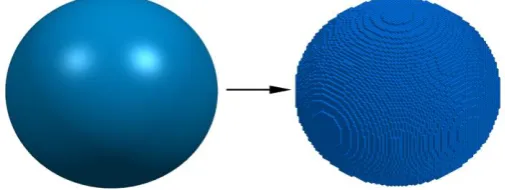
Figure 1. Finite difference grid (FDM grid).

Two common methods for large-scale FDM grid generation are ray casting method and slicing method. Ray casting method creates rays and computes the intersection between rays and geometries [14]. This method has been widely applied to large-scale grid generation because of the clear procedure, but the step of intersection calculation cost too much time. Slicing algorithm [15], which is similar with the slicing method in rapid prototyping machining [16, 17], cut the geometries using a series of parallel planes and construct contours in each plane. Then, the grid will be generated in each slicing plane. This method reduces time cost in geometry intersection calculating and has a higher efficiency in most cases. However, the topological reconstruction is necessary to slicing algorithm and cost extra time. Because the boundary of each geometry in the finite difference grid has a ladder shape, increasing grid scale is an efficient means to eliminate the error caused by the mismatch between the grid boundary and the real boundary. At least millions of grids are usually required in three-dimensional FDM simulation, which leads to the generation of FDM grid cost a large time to guarantee the accuracy of simulation. How to shorten time of grid generation is one of hot spots all the time. Jeff T. MacGillivary [18] achieve trillion Cartesian grid generation with a novel ray-facet intersection test and a efficient data storage method. But the phenomenon of geometric degeneration still needs to be improved.

In this paper, the ray casting algorithm is optimized and some special cases of algorithm are analyzed, which improve the efficiency and stability for large-scale grid generation. The facet search method of traditional ray casting algorithm is modified to improve the performance of intersection calculation. An efficient data storage method is proposed for storing and visualizing grid data, which makes it possible to display trillions of grid in Section 2. The advantage of modified ray casting algorithm is discussed through performance comparison between ray casting and slicing method in different situations in Section 3. Finally, examples of grid generation and explosion simulation are presented. The accuracy of algorithm is proved.

Theory

In the past decades, ray casting algorithm is the most popular and accurate method for generating FDM grid. Ray casting algorithm can generate large-scale grids through a simple procedure, and has higher stability and parallelism. The ray casting algorithm contains 4 main steps: ray generation, intersection judgment, intersection calculation and data visualization. In the following section, the inefficient and low accuracy parts in each step will be modified or optimized to improve the performance and stability of integral algorithm.

Input File

Ray Generation

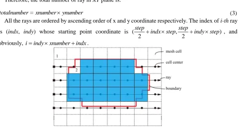
Suppose that the computational domain is a cuboid region as shown in Fig. 2. The computational domain can be fixed by two points: P1 (xmin，ymin，zmin), P2 (xmax，ymax，zmax). All the geometries in computational domain will be meshed. A ray direction is chosen, which is usually the maximum in three dimensional directions, such as z direction in Figure. 2. Then, in the plane which is perpendicular to the ray direction, such as XY plane, starting points of rays are generated. Each ray passes through the whole computational domain to reach its ending point, such as the ray in Fig. 2. According to the step of grid, a series of rays are generated distributed in all computational domain. Taking the uniform grid as an example, the ray number in x direction is:

( )

xnumber xmaxxmin step (1) Similarly, the ray number in y direction is:

( )

ynumber xmaxxmin step (2) Therefore, the total number of ray in XY plane is:

totalnumber = xnumberynumber (3) All the rays are ordered by ascending order of x and y coordinate respectively. The index of i-th ray

is (indx, indy) whose starting point coordinate is ( , )

2 2

step step

indx step indy step

    , and

obviously, iindyxnumberindx.

Figure 2. Distribution of ray in XY plane.

Intersection Judgment

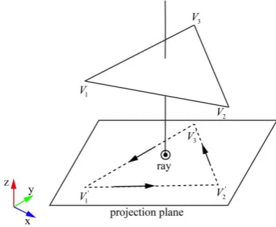
In three-dimensional space, rays cross the whole computational domain. Some facets that form geometries may be intersected with the ray and some may be not. In order to calculate the intersection point between ray and facets, it is necessary to judge which facet could intersect with ray firstly. A judgment method without division calculation is used, which can reduce the machine error. For a ray

r and a facet t, v1, v2, v3, are three vertexes of t. The Orientation represents the relative location can

be calculated as Equation 4:

1 1

2 2

x y y

x y y

v r v r

Orientation

v r v r

 



  (4)

where Orientation represents the relative location of the edge v v_{1 2} and ray r. If Orientation > 0, r is

located on the left side of edge v v_{1 2}. Whereas, If Orientation < 0, r is located on the right side of edge

1 2

the ray r pass through the interior of facet t if the following condition is satisfied: all three

Orientations are greater than 0 or all three Orientations are less than 0. As Fig. 3 shown, there is a ray crossing over a facet whose vertexes are V₁, V₂, V₃. V₁', V₂', V₃' are vertexes projected in XY plane.

The location of starting point of ray is on the left side for all three edges V V₁' ₂', V V₂' ₃' and V V₃' ₁'.

Figure 3. Ray casting algorithm.

Modified Facet Search Method

Figure 4. Search tree of facet.

Calculating Intersection Point

According to judgment in section 2.3, some facets which intersect with ray r can be obtained. All intersections can be computed as Equation 5. Intersection points are sorted as r direction and stored in point set P.

1 1 1

2 1 2 1 2 1 0

3 1 3 1 3 1

x x y y z z

x x y y z z

x x y y z z

r v r v r v

v v v v v v

v v v v v v

  

   

  

(5)

Degenerate Detection

In three-dimensional space, seven possible relationships between a ray and a facet are: crossing, missing, crossing point, crossing edge, parallel, coplanar nonintersecting and coplanar intersecting. Obviously, crossing and missing can be calculated correctly through the above method. However, the other situations may be judged incorrectly, and are discussed as below.

As stated above, three orientations O1, O2, O3 are indicated the relationship between a ray and a

facet. Crossing point is that a situation that a ray crossing a vertex. At the same time, because that the geometry is closed, the ray must also crossing the vertex which belongs to other facets. In this case, Two orientations equal to 0, and the other one must be not 0. This situation can be calculated correctly, but the same point must be reserved only once. Crossing edge is that a ray crossing an edge. Similarly, one of orientations must be 0, and others must be positive or negative at the same time. Two same intersection points can be calculated through different facets and only one will be reserved. When a ray is parallel to a facet, the three orientations cannot be positive or negative at the same time. As a result, this relationship will be judged as missing, which is consistent with the facts. When a ray is coplanar but does not intersect a facet, all three orientations must be 0. It is true that the relationship will be judged to be missing. For the last situation, a ray is coplanar with a facet and passes through it. All three orientations must be 0. In this case, the face must be part of the geometry boundary, where the face cannot contain meshes. Therefore, the missing facts can be correctly calculated.

algorithm [22]. However, the machine accuracy is enough for our grid generation application. Exact arithmetic algorithm is not used considering the efficiency.

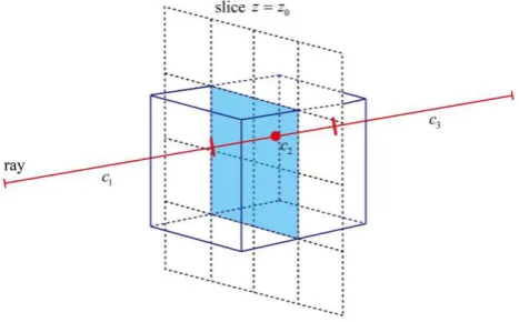
Storage and Visualization of Large-Scale Data

The scale of FDM grid in three-dimensional space is usually very large. Large amount of data for computing and storage require huge memory and hard disk capacity. Reasonable data structure can avoid the problem of storage. In method presented, there is no grid point data stored in memory. The only data stored is triangular facets and intersection points in a ray. After computing intersection points of the current ray, data is written to disk, memory is free, and the next ray is read to compute. Therefore, the program can run using a very small memory space. After computing the ordered intersection set P, the length between each intersection points should be calculated and a length set L

is obtained. All the elements in L are divided by the grid step, and the set C is obtained. The set of positive integers C is the only data written to the disk for a ray. The number of element in C only depends on geometry. Generally, there is a small disk capacity needed for large scale FDM grid.

There is a large number of graphic vertexes when a FDM grid is rendered in three-dimensional space. It is impossible to render billions of vertexes in the current hardware environment. Therefore, slicing display is an appropriate method. Through above operation, an integer set C is obtained and stored in disk for every ray. Elements in C represents grid number of different materials. Every row in file stores a set C corresponding to a ray. For each row, even numbered integer represent the grid number in geometry and odd numbered integer represent the grid number out of geometry, as Fig. 5 shown.

Figure 5. The process of rendering a slice.

Suppose that grids in slice z z₀ need to be displayed, we calculate whether z₀ located in even segment for each row in file or not. If z₀ located in even segment, the grid is rendered in the same color of geometry. Pseudo code of this procedure is as follow, where xnumber represents grid number in x direction, ynumber represents grid number in y direction, and cnumber represents element number of set C for each ray:

x ← 0, y ← 0, flag ← 0; while (y < ynumber) {

while (x < xnumber) {

while (i < cnumber) {

if (z0 > 0

i

i n



if (flag ← 1)

The grid is inside of geometry; else

The grid is outside of geometry; x ← x+1;

}

y ← y+1; }

Similarly, all three views can be rendered based slices in each direction. The result of generation can be inspected through the three views and each slice. For multiple geometries, The only different operation is to take the same operation on the file of each geometry.

In summary, 3 steps of ray casting algorithm are optimized in this paper as follows: 1. A search tree is built to improve the efficiency of facet search;

2. All cases of intersection in 3 dimension space are analyzed to improve the accuracy of algorithm; 3. A slicing display method is proposed to make the visualization of trillion grids possible.

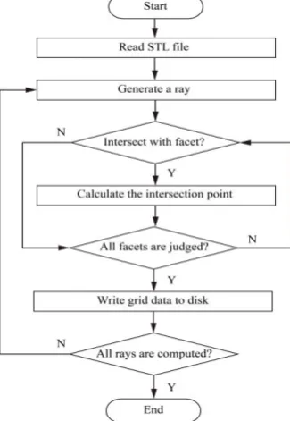
The general procedure of modified ray casting algorithm can be shown as a flowchart in Fig. 6.

Figure 6. Flow chart of ray casting algorithm procedure.

Result and Discussion

A Result of Fdm Grid Generation

Figure 7. Result of a large-scale grid from a large STL file.

Discussion about Two Algorithms

In this section, ray casting algorithm is compared with slicing algorithm in theory. Performance of algorithm and memory usage are two main aspects discussed.

The process of ray casting algorithm is simpler than slicing algorithm. As Fig. 6 shown, the total number of iterations is the number of rays, which can be expressed as:

xynumber = xnumberynumber. Then, in every iteration, intersection judgment is calculated for each ray. In traditional ray casting algorithm, the time of judgment is the number of facets in STL file

stlnumber. Therefore, the complexity of the whole algorithm is O(xynumber*stlnumber). Because of the facet search method presented in section 2.4, the time of judgment decrease greatly, which depends on the deep of tree and the distribution of facets. Based on the principle of binary tree, the complexity of the modified ray casting algorithm can reach O(xynumber*logstlnumber) in the best case.

In this section, the performance of modified algorithm in different situation is evaluated through an example.

Figure 8. Comparison of modified algorithm and the old one.

Slicing algorithm contains two main steps: slicing and calculating intersection in 2 dimension space. Details of slicing algorithm is presented in [4]. In the first step, the number of iteration is

znumber, calculating intersection points between slice and geometry every time. In the second step,

ynumber iteration is carried out to calculate the intersection in a slice. So the total complexity of algorithm is O(ynumber×znumber), which means the time consumption of algorithm only depends on the total number of grid in YZ plane. It looks like that there is no difference in two algorithm. However, there is an additional operation taken in slicing algorithm. Slicing generation is a necessary step in slicing algorithm, whose efficiency depends on the complexity of geometry. The more triangular facets the geometry contains, the more time will be cost for slicing algorithm. However, additional operation bring convenience when intersection points are calculated. Because some multiplication calculations are converted into additive calculations, the efficiency of calculating intersection points will be greatly improved.

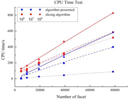
A comparison of performance between the modified ray casting algorithm and slicing algorithm is presented in Fig. 9. The CPU times of generating different number of grid using two algorithms are presented with the same 3D models as above section. The red color represents the slicing algorithm and the blue color represents the modified ray casting algorithm. The square, circle and triangular symbol represents the quantity of grid generated.

Figure 9. Comparison of ray casting algorithm and slicing algorithm.

two different trends: the slicing algorithm represented by blue line exhibits a linear change with the number of facet, and the change with the number of facet using modified ray casting algorithm conforms to a logarithmic function. Therefore, with the increasing of facets number, the performance of ray casting algorithm will be much greater than the performance of slicing algorithm.

In each iteration, the main calculation of ray casting algorithm needs a ray and all the triangular facets. Therefore, the data stored in memory contains the start point of ray, vertex coordinates of facets and some intersection points calculated. Usually, the start point of ray and intersection points have very small size which can be ignored. The memory usage of ray casting algorithm is determined by number of triangular facet. Similarly, slicing algorithm need all the triangular facets. However, the whole grid data in a slice also need to be stored in memory. The grid data in a slice is increasing with the scale of grid, whose complexity can be expressed as O(xynumber).

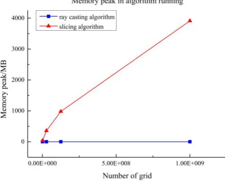
A memory test is done and the memory peak in algorithm running of two algorithms is recorded in Fig. 10. The memory peak of ray casting algorithm is maintained a constant value with the increase of grid number. However, the memory peak of slicing algorithm rapidly rise with the increase of grid number. Further, Fig. 11 shows the memory peak of slicing algorithm is directly proportional to

gridnumber2/3. The test is consistent with the theoretical analysis.

Figure 10. Comparison in Memory peak of two algorithms.

A Result of Explosion Simulation

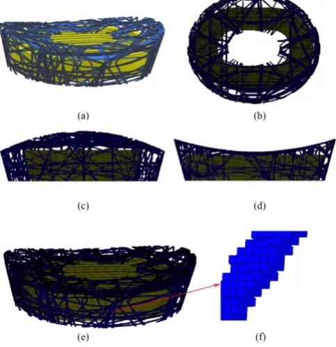
In this part, we present a result of a simulation of the explosion in a Stadium. As Fig. 12 shown, the computational domain contains 4 materials: air, explosive, grandstand, and main structure of stadium. The total number of mesh is 1.5×109. The CPU time cost 180.34s in the complete procedure of mesh generation.

Figure 12. A mesh generation result of a stadium model.

We completed the simulation using the Eulerian three-dimensional multi-material parallel hydrocode PMMIC-3D [23] and the result is shown in Fig. 13 (a). The factory is represented by blue color, and the detonation products of the explosive is represented by red color. TNT is detonated in the grandstand of stadium. It can be easily observed how the shock wave creating and propagating in the air. It is of great practical significance in explosion protection.

Conclusions

In this paper, the algorithm of ray casting is optimized and achieved in generating FDM grid. A variety of degenerated case are analyzed and some judgments are added to ensure the efficiency and stability of algorithm. Aiming at large scale FDM grid generation, an efficient data storage method is proposed for using memory more reasonable. The method of visualizing grid data in slice is presented to make it possible to display trillions of grid.

Slicing algorithm and modified ray casting algorithm are analyzed and compared in theory and experiment. The advantages of ray casting algorithm is presented. Through the examples of FDM grid generation and the simulation of factory explosion, the modified ray casting algorithm is proved that it can be well applied to finite difference calculation.

Acknowledgement

This work was supported by the National Natural Science Foundation of China (Grant Nos. 11772061 and 11822203), and project of State Key Laboratory of Explosion Science and Technology (Grant No. YBKT 18-01).

References

[1] J. Ning, H. Ren, T. Guo, et al., Dynamic response of alumina ceramics impacted by long tungsten projectile, International Journal of Impact Engineering, 2013, 62, pp. 60-74.

[2] J Ning, W. Song, and G. Yang, Failure analysis of plastic spherical shells impacted by a projectile, International Journal of Impact Engineering, 2006, 32(9), pp. 1464-1484.

[3] J. Li, J. Ning, and J. H. S. Lee, Mach reflection of a ZND detonation wave, Shock Waves, 2015, 25(3), pp. 293-304.

[4] J. Li, H. Ren, X. Wang, et al., Length scale effect on Mach reflection of cellular detonations, Combustion & Flame, 2017, 189

[5] J. Li, H. Ren, and J. Ning, Numerical application of additive Runge-Kutta methods on detonation interaction with pipe bends, International Journal of Hydrogen Energy, 2013, 38(21), pp. 9016-9027.

[6] J. Ning and L. Chen, Fuzzy interface treatment in Eulerian method, Science in China Series E-Engineering & Materials Science, 2004, 47(5), pp. 550-568.

[7] J. Zhu and M. Gotoh, An automated process for 3D hexahedral mesh regeneration in metal forming, Computational Mechanics, 1999, 24(5), pp. 373-385.

[8] Z. Q. Xie, R. Sevilla, O. Hassan et al., The generation of arbitrary order curved meshes for 3D finite element analysis, Computational Mechanics, 2013, 51(3), pp. 361-374.

[9] J. Ning, T. Ma, and G. Lin, A mesh generator for 3-D explosion simulations using the staircase boundary approach in Cartesian coordinates based on STL models, Advances in Engineering Software, 2014, 67(1), pp. 148-155.

[10] B. Roget and J. Sitaraman, Robust and efficient overset mesh assembly for partitioned unstructured meshes, Journal of Computational Physics, 2014, 260(1), pp. 1-24.

[11] D. Dezeeuw and K. G. Powell, an Adaptively Refined Cartesian Mesh Solver for the Euler Equations, Journal of Computational Physics, 1991, 104(1), pp. 56-68.

[13] S. Park and H. Shin, Efficient generation of adaptive Cartesian mesh for computational fluid dynamics using GPU, International Journal for Numerical Methods in Fluids, 2012 70(11), pp. 1393-1404.

[14] Y. Srisukh, J. Nehrbass, F. L. Teixeira, et al., An approach for automatic grid generation in three-dimensional FDTD simulations of complex geometries, IEEE Antennas & Propagation Magazine, 2002, 44(4), pp. 75-80.

[15] Q. Qin, C. Hu, and T. Ma, Study on complicated solid modeling and Cartesian grid generation method, Science China Technological Sciences, 2014, 57(3), pp. 630-636.

[16] P. M. Pandey, N. V. Reddy, and S. G. Dhande, Slicing procedures in layered manufacturing: a review, Rapid Prototyping Journal, 2003, 9(5), pp. 274-288.

[17] A. Bahram and K. Behrokh, Machine path generation for the SIS process, Robotics and Computer-Integrated Manufacturing, 2004, 20(3), pp. 167-175.

[18] J. T. Macgillivray, Trillion Cell CAD-Based Cartesian Mesh Generator for the Finite-Difference Time-Domain Method on a Single-Processor 4-GB Workstation, IEEE Transactions on Antennas & Propagation, 2008, 56(8), pp. 2187-2190.

[19] M. Szilvi-Nagy and S. G. ty, Analysis of STL files, Mathematical & Computer Modelling, 2003, 38(7), pp. 945-960.

[20] M. Kolosovskiy, Simple implementation of deletion from open-address hash table, Computer Science, 2009.

[21] J. Bonet and J. Peraire, An alternating digital tree (ADT) algorithm for 3D geometric searching and intersection problems, International Journal for Numerical Methods in Engineering, 1991, 31(1), pp. 1-17

[22] J. R. Shewchuk, Adaptive Precision Floating-Point Arithmetic and Fast Robust Geometric Predicates, Discrete & Computational Geometry, 1997, 18(3), pp. 305-363.