© 2015, IRJET ISO 9001:2008 Certified Journal
Page 1148
To Analysis the performance of two area power system in Automatic
Generation Control based on MATLAB
Anupam Mourya
1, Rajesh kumar
2, Sanjeev Kumar
3, Dr. Manmohan Singh
41
M.Tech Scholar, Electrical Engineering, Yamuna Institute of Eng. & Tech, Yamuna Nagar, Haryana, India
2Assistant Prof., Electronic and Communication Engineering, Shoolini University, Himachal Pradesh, India
3Assistant Prof
, Electrical Engineering, Yamuna Institute of Eng. & Tech, Yamuna Nagar, Haryana, India
4Assistant Prof,
Electrical & Instrumentation Engineering, Sant Longowal University Sangrur, Punjab, India
---***---Abstract
- The main objective of this paper is to study the load frequency control problem associated in single and Two-area electrical power systems. At first uncontrolled system is studied and then improvement of its response is learnt on the application of integral controller. All the study is done using MATLAB software both in SIMULINK and Workspace windows. By comparing the simulation of controller and workspace controller results obtained. By using Matlab Software, a good agreement between these results is obtained. Thus the response of Two area power system with integral controller is suitable than response of other controllers availableKey Words:
Power system control, AGC,
Parameter
calculations, Load frequency control, Integral
Controller, SIMULINK and Workspace, MATLAB
1. INTRODUCTION
The main purpose of operating the load frequency control is to keep uniform the frequency changes during the load changes. During the power system operation rotor angle, frequency and active power are the main parameters to change. In multi area system a change of power in one area is met by the increase in generation in all areas associated with a change in the tie-line power and a reduction in frequency. In the normal operating state the power system demands of areas are satisfied at the nominal frequency. A simple Control strategy for the normal mode is to operate in such a way that to keep frequency approximately at nominal value, Maintain the tie-line flow at about schedule, each area should absorb its own load changes. Controller must be sensitive against changes in frequency and load. To analyze the control system mathematical model must be established. There are two models which are widely used, 1. Transfer function model 2. State variable approach. The most applied controller is Conventional Integral (PI), So that the power system operations, the load is changing continuously and randomly. As a result the real and reactive power demands on the power system are never steady, but continuously vary with the rising or falling
trend. The real and reactive power generations must change accordingly to match the load perturbations. Load frequency control is essential for successful operation of power systems, especially interconnected power systems [13]. Without it the frequency of power supply may not be able to be controlled within the required limit band. To accomplish this, it becomes necessary to automatically regulate the operations of main steam valves or hydro gates in accordance with a suitable control strategy, which in turn controls the real power output of electric generators. The problem of controlling the output of electric generators in this way is termed as Automatic Generation Control (AGC) [14]. Automatic generation control is the regulation of power output of controllable generators within a prescribed area in response to change in system frequency, tie-line loading, or a relation of these to each other, so as to maintain the schedule system frequency and/or the established interchange with other areas within predetermined limits [13].Automatic Generation Control can be sub divided into fast (primary) and slow (secondary) control modes. The loop dynamics following immediately upon the onset of the load disturbance is decided by fast primary mode of AGC. This fast primary mode of AGC is also known as “Uncontrolled mode” since the speed changer position is unchanged. The secondary control acting through speed changer and initiated by suitable controller constitutes the slow secondary or the “Controlled modes” of AGC. The overall performance of AGC in any power system depends on the proper design of both primary and secondary control loops. So the overall performance of AGC in any power system depends on the proper design of both primary control loop (selection of R) and secondary control loops (selection of gain for supplementary controller).
Among the various types of load frequency controllers, the most widely employed are integral (I), their use is not only for their simplicity, but also due their success in large industrial applications
© 2015, IRJET ISO 9001:2008 Certified Journal
Page 1149
To understand the load frequency control problem, let usconsider a single turbo-generator system supplying an isolated load.
For LFC scheme of single generating unit has basically three parts:
Turbine speed governing system Turbine Generator and
load
In the next section, mathematical transfer function model of single area thermal system is developed.
2.1 Turbine Speed Governing System Model
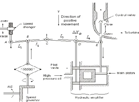
Fig. 2.1 shows schematically the speed governing system of a steam turbine. The system consists of the following components:
(1) Fly ball speed governor: This is the heart of the system which senses the change in speed (frequency). As the speed increases the fly balls move outwards and the point B on linkage mechanism moves downwards. The reverse happens when the speed decreases.
[image:2.595.39.278.447.622.2](2) Hydraulic amplifier: It comprises a pilot valve and main piston arrangement. Low power level valve movement is converted into high power level piston valve movement. This is necessary in order to open or close the steam valve against high pressure steam.
Fig. 2.1 Model of Turbine speed governing system
(3) Linkage mechanism: ABC is a rigid link pivoted at B and CDE is another rigid link pivoted at D. This link mechanism provides a movement to the control valve in proportion to change in speed. It also provides a feedback from the steam valve movement.
(4) Speed changer: It provides a steady state power output setting for the turbine. Its downward
movement opens the upper pilot valve so that more steam is admitted to the turbine under steady conditions (hence more steady power output). The reverse happens for upward movement of speed changer.
Let the point A on the linkage mechanism be moved downwards by a small amount ∆yA. It is a command which causes the turbine power output to change and can therefore be written as
∆yA=KC∆PC (2.1) Where ∆PC is the commanded increase in power:
The command signal ∆PC (i.e. ∆yE) sets into motion a sequence of events - The pilot valve moves upwards, high pressure oil flows on to the top of the main piston moving it downwards; the steam valve opening consequently increases, the turbine generator speed increases, i.e. the frequency goes up. Let us model these events mathematically.
Two factors contribute to the movement of C:
(1) ∆yA contributes- 2 1
A
L
y
L
or –K1∆yA (i.e. upwards) of
K K
1 C
P
C(2) Increase in frequency ∆f causes the fly balls to move outwards so that B moves downwards by a proportional amount
K
'
2
f
. The consequentmovement of C with A remaining fixed at ∆yA is
2 2
2 2
1
'
L
L
K
f
K
f
L
(i. e. downwards)The net movement of C is therefore
y
CK K
1 C
P
CK
2
f
(2.2) The movement of D, ∆yD, is the amount by which the pilotvalve opens. It is contributed by ∆yC and ∆yE and can be written as
4 3
3 4 3 4
D C E
L
L
y
y
y
L
L
L
L
=K3∆yC + K4∆yE (2.3) The movement ∆yD depending upon its sign opens one of
the ports of the pilot valve admitting high pressure oil into the cylinder thereby moving the main piston and opening the steam valve by ∆yE.
The volume of oil admitted to the cylinder is proportional to the time integral of ∆yd. The movement ∆yE is obtained by dividing the oil volume by the area of the cross section of the piston. Thus
∆yE= 5
0
(
)
t D
k
y
dt
(2.4) Take Laplace transform of Eqs. (2.2), (2.3) and (2.4),© 2015, IRJET ISO 9001:2008 Certified Journal
Page 1150
51
( )
( )
E D
Y s
K
Y s
s
Eliminating ∆YC(s) and ∆YD(s), we can write
1 3 2 3
4 5
( ) ( )
( ) C C
E
K K K P s K K F s
Y s s K K 1 ( ) ( ) 1 sg C sg K
P s F s
R T s
(2.5)
Where 1 2
C
K K
R
K
= speed regulation of the governor1 3 4
C sg
K K K
K
K
= gain of speed governor4 5
1
sgT
K K
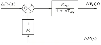
= time constant of speed governor [image:3.595.35.285.161.340.2]The equation can be represented in the form of a block diagram in Fig. 2.2.
Fig. 2.2 Block diagram representation of speed governor system
2.2 Turbine Model
The dynamic response is largely influenced by two factors, (i) entrained steam between the inlet steam valve and first stage of the turbine, (ii) the storage action in the reheater which causes the output if the low pressure stage to lag behind that of the high pressure stage. Thus, the turbine transfer function is characterized by two time constants. For ease of analysis it will be assumed here that the turbine can be modeled to have a single equivalent time constant as given in Fig. 2.3
Fig. 2.3 Turbine transfer function model
Where, Kt = Gain of turbine, Tt = Time constant of turbine
2.3 Generator Load Model
The increment in power input to the generator-load system is
∆PG - ∆PD
Where ∆PG = ∆Pt, incremental turbine power output (assuming generator incremental loss to be negligible) and ∆PD is the load increment.
This increment in power input to the system is accounted for in two ways:
(1) Rate of increase of stored kinetic energy in the generator rotor. At scheduled frequency (fº), the stored energy is
0
ke r
W
H
P
kW = sec (kilojoules)Where Pr is the kW rating of the turbo-generator and H is defined as its inertia constant.
The kinetic energy being proportional to square of speed (frequency), the kinetic energy at a frequency of (fº + ∆f) is given by 2 0 0 0 ke ke f f W W f 0 2 1 r f HP f (2.6)
Rate of change of kinetic energy is therefore
2
0r(
)
keHP
d
d
W
f
dt
f
dt
(2.7)(ii) As the frequency changes, the motor load changes being sensitive to speed, the rate of change of load with respect to frequency, i.e. ∂PD/∂f can be regarded as nearly constant for small changes in frequency ∆f and can be expressed as
P
Df
B f
f
(2.8) Where, the constant B can be determined empirically. B ispositive for a predominantly motor load. Writing the power balance equation, we have
2
0r(
)
G D
HP d
P
P
f
B f
f
dt
Dividing throughout by Pr and rearranging, we get
0
2
( ) ( ) ( ) ( )
G D
H d
P pu P pu f B pu f
f dt
(2.9)
Taking the Laplace transform, we can write ∆F(s) as 0 ( ) ( ) ( ) 2 G D
P s P s
F s H B s f =
( ) ( )
1 G D KpsP s P s
[image:3.595.71.247.400.479.2]© 2015, IRJET ISO 9001:2008 Certified Journal
Page 1151
T
ps2
H
0Bf
= power system time constant
K
ps1
B
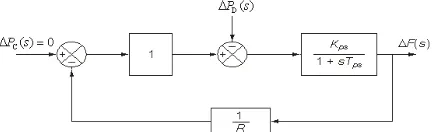
= power system gain [image:4.595.100.257.220.274.2]The equation can be represented in block diagram form as in Fig. 2.4.
Fig. 2.4 Block diagram representation of generator-load model
3. Block Diagram Representation of Load
Frequency Control of an Isolated Area
A block diagram representation of an isolated power system by combining the block diagrams of turbine, generator, governor and load with feedback loop as shown in Fig. 3.1
Fig. 3.1 Block Diagram Model of Load Frequency Control (isolated power system)
3.1 Steady States Analysis
The model of Fig. 3.1 shows that there are two important incremental inputs to the load frequency control system i.e. -∆PC, the change in speed changer setting; and ∆PD, the change in load demand. Let us consider the speed changer has a fixed setting (i.e. ∆PC =0) and load demand changes. This is known as free governor operation. For such an operation the steady change in system frequency for a sudden change in load demand by an amount ∆PD (i.e ∆PD(s) = ∆PD/s) is obtained as follows
( ) 0
( ) ( ) |
/
(1 )
(1 )(1 )
C
ps D
P s
sg t ps
ps
sg t
K P s
F s
K K K R s
T s
T s T s
(3.1)
│∆fsteady state = s∆F(s) │
1 ( / )
ps
D sg t ps
K
P K K K R
(3.2)
│∆PC = 0
s
0
∆PC(s) = 0│
Let it be assumed for simplicity that Ksg is so adjusted that KsgKt ≈ 1
It also recognized that Kps = 1/B, where B = (∂PD/∂f) / Pr (in pu MW/unit change in frequency). Now
1
1 D
f P
B R
[image:4.595.312.551.238.400.2](3.3)
Fig. 3.2 Steady State LFC characteristics of a speed governor system
Fig. 3.2 shows the linear relationship between frequency and load for free governor operation with speed changer set to give a scheduled frequency of 100% at full load. It depicts two load frequency plots – one to give scheduled frequency at 100% rated load and the other to give the same frequency at 60% rated load
The ‘droop’ or slope of this relationship is
1
1
B
R
.
Consider now the steady effect of changing speed changer setting
( )
CC
P
P s
s
with load demand remaining fixed (i.e. ∆PD = 0). The steady state change in frequency is obtained as follows.( ) 0 ( )
(1 )(1 )(1 )
D
sg t ps C
sg t ps P s
sg t ps
K K K P
F s
K K K s T s T s T s
R
(3.4)
1 0
sg t ps
C
sg t ps
D
steady state P
K K K
f P
K K K R
[image:4.595.39.253.426.531.2]© 2015, IRJET ISO 9001:2008 Certified Journal
Page 1152
1
1 C
f P
B R
(3.5)
If the speed changer setting is changed by ∆PC while the load demand changes by ∆PD the steady frequency change is obtained by superposition, i.e.
1
( )
1 C D
f P P
B R
(3.6)
From Eq. (3.6) the frequency change caused by load demand can be compensated by changing the setting of the speed changer, i.e. ∆PC = ∆PD, for ∆f =0
3.2 Dynamic Response
To obtain the dynamic response giving the change in frequency as function of the time for a step change in load, we must obtain the Laplace inverse of Eq. (3.1). The characteristic equation can be approximated as first order by examining the relative magnitudes of the time constants involved. Typical values of the time constants of load frequency control system are related as
Tsg << Tt <<Tps
[image:5.595.311.550.273.405.2]Consider Tsg=0.08 sec, Tt=0.3 sec., and Tps=20 sec
Fig. 3.3 first order approximate block diagram of load frequency control of an isolated area
Letting Tsg = Tt = 0, (and KsgKt ≈ 1), the block diagram of Fig. 3.1 is reduced to that of Fig.3.3, from which we can write
( ) 0
( )
1
/ =
ps D
ps c
ps
ps ps
D ps ps
P s
K P
F s
K s
T s R
K T
P
R K
s s RT
( ) ps 1 exp ps D
ps ps
RK t R K
f t P
R K T R
(3.7)
Taking R=2.4, Kps=120, Tps=20 sec., ∆Pd =0.01 pu
∆f (t) = -0.0235(1- 2.55t
e
) (3.8)∆steady state = - 0.0235 Hz
4 SIMULINK Model
A SIMULINK model named sm_A1_wc is constructed for isolated uncontrolled power system as shown in Fig. 4.1
DPc (s)
Turbine 1 0.3s+1
To Workspace simout Speed Governor
1 0.08 s+1
Scope Generator
120 20 s+1 DPd (s)
[image:5.595.40.261.478.544.2]1/R 1/2.4
Fig. 4.1 SIMULINK model for uncontrolled isolated area
4.1 Control Area Concept
It is possible to divide an extended power system (say, national grid) into sub areas (may be, state electricity boards) in which the generators are tightly coupled together so as to form a coherent group, i.e. all the generators respond in unison to changes in load or speed changer settings. Such a coherent area is called a control area in which the frequency is assumed to be the same throughout in static as well as dynamic conditions. For purposes of developing a suitable control strategy, a control area can be reduced to single speed governor, turbo-generator and load system.
4.2 Application of Integral Controller
© 2015, IRJET ISO 9001:2008 Certified Journal
Page 1153
4.3Two-Area Load Frequency Control
4.3.1 Introduction
[image:6.595.308.550.137.227.2]The large-scale power systems are normally composed of control areas (i.e. multi-area) or regions representing coherent groups of generators. The various areas are interconnected through tie-lines. The tie-lines are utilized for contractual energy exchange between areas and provide inter-area support in case of abnormal conditions. Without loss of generality we shall consider a two-area case connected by a single line as illustrated in Fig. 4.4. The concepts and theory of two-area power system is also applicable to other multi-area power systems i.e. three-area, four-three-area, five-area etc.
Fig. 4.3 Two interconnected control areas (single tie line)
Power transported out of area 1 is given by
0 0
1 2
, 1 1 2
12
|
||
|
sin(
)
tie
V
V
P
X
(4.1)Where
1,
2= power angles (angle between rotating magnetic
flux & rotor) of equivalent machines of the two areas.For incremental changes in f1 and f2, the incremental tie line power can be expressed as
Ptie,1(pu) = T12(1-2) (4.2)
Where
0 0
1 2
12 1 2
1 12
|
||
|
cos(
)
r
V
V
T
P X
= synchronizing coefficientSince incremental power angles are integrals of incremental frequencies, we can write above Eq. (4.2) as
, 1
2
12 1 2tie
P
T
f dt
f dt
(4.3)Where, f1 and f2 are incremental frequency change of areas 1 and 2 respectively.
Similarly the incremental tie line power out of area 2 is given by
, 2
2
21 2 1tie
P
T
f dt
f dt
(4.3)
Where
0 0
2 1 1
21 2 1 12 12 12
2 21 2
|
||
|
cos(
)
rr r
V V
P
T
T
a T
P X
P
(4.4)
With ref. to Eq. (2.9), the incremental power balance equation for area1 can be written as
1
1 1 0 1 1 1 1
1
2
(
)
,
G D
H d
P
P
f
B f
Ptie
f
dt
(4.5)It may be noted that all quantities other than frequency are in per unit in Eq. (4.5).
Taking the Laplace transform of Eq. (4.5) and reorganizing, we get and show the block diagram in fig 4.4
1
1 1 1 1
1
( ) [
( )
( )
, ( )]
1
G D
Kps
F s
P s
P s
Ptie
s
Tps S
(4.6)Fig.4.4 Turbine-Load Model for Two-Area LFC & Model Corresponding to Tie line Power Change
Taking the Laplace transform of Eq. (4.6), the signalPtie,1
(s) is obtainedas
12
, 1 1 2
2
( )
[
( )
( )]
tie
T
P
s
F s
F s
s
(4.7)The corresponding block diagram is shown in Fig. 4.4.
For the control area 2, Ptie, 2(s) is given as
12 12
, 2 1 2
2
( )
[
( )
( )]
tie
a T
P
s
F s
F s
s
(4.8) [image:6.595.39.283.306.359.2]© 2015, IRJET ISO 9001:2008 Certified Journal
Page 1154
In the case of an isolated control area, ACE is the change inarea frequency which when used in integral control loop forced the steady state frequency error to zero. In order that the steady state tie line power error in a two-area control be made zero another control loop (one for each area) must be introduced to integrate the incremental tie line power signal and feed it back to speed changer. For the control area 2, ACE2 is expressed as
ACE2(s) = Ptie,2(s) + b2 F2(s) (4.9)
Where b constant
4.4 Block Diagram of Uncontrolled Two-Area LFC
[image:7.595.312.562.103.209.2]Block diagram of uncontrolled two-area power system is given in Fig. 4.5.
Fig. 4.5.Block diagram of two-area load frequency control without controller
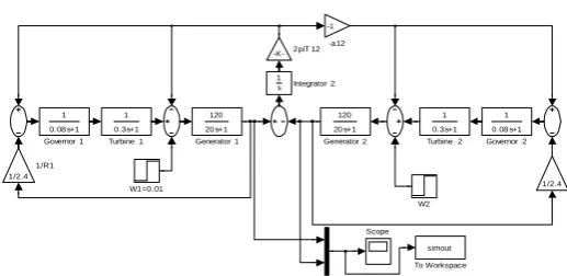
4.4.1 SIMULINK Model for Uncontrolled Two-Area
LFC
W2 W1=0.01
Turbine 2 1 0.3s+1 Turbine 1
1 0.3s+1
To Workspace simout Scope Integrator 2 1 s
Governor 2 1 0.08 s+1 Governor 1
1 0.08 s+1
Generator 2 120 20 s+1 Generator 1
120 20 s+1
2piT 12
-K-1/R2 1/2.4 1/R1
1/2.4
-a12 -1
Fig. 4.6 SIMULINK model for two-area LFC without using controller
4.5 Block Diagram of Two-Area LFC with Integral
Controller
Block diagram model and its corresponding diagram to derive state space model of two-area LFC with integral controller are given in Fig. 4.7 (a) and (b) respectively.
Fig. 4.7 (a) Block diagram of two-area LFC with Integral controller
4.5.1 SIMULINK Model for Two-Area LFC with
Integral Controller
[image:7.595.311.564.305.429.2]A SIMULINK model named sm_A2_I is constructed as showninFig.4.8
Fig. 4.8 SIMULINK model of two-area LFC with Integral controller
5 Results and Discussion
5.1Two-Area Power System
Simulations Models were performed with uncontroller and with integral controller is applied to two-area electrical power system by applying 0.01 p.u. MW step load disturbance to area 1
5.2 Two-Area Power System without controller
[image:7.595.39.280.307.402.2] [image:7.595.37.296.469.595.2]© 2015, IRJET ISO 9001:2008 Certified Journal
Page 1155
0 5 10 15 20 25 30
-0.025 -0.02 -0.015 -0.01 -0.005 0
Time (sec.)
D
el
ta
f1
(
pu
),D
el
ta
f2
(
pu
)
Two-area LFC without controller
Delta f1 Delta f2
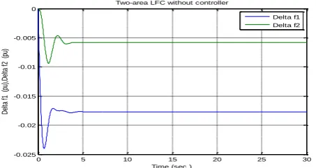
Fig.5.1.Result of Two Area LFC without Integral controller
This fig. 5.1 shows Controlled Two Area power system without Integral controller, It shows the relationship between power unit and frequency( 1/time) for two power system .The Power Unit is high at time zero second, oscillation will produce till time five second after that it damped out i.e. become study state, It mean frequency of load controlled
5.2 Two-Area Power System with Integral
Controller
From the responses of the Figs. 4.1 and 4.3 we observe that both responses match with each other and steady state frequency deviation is zero, and the frequency returns to its nominal value in approximately 13.5 seconds.Results are shown in Table-1
Fig.5.2.Result of Two area LFC with Integral controller
The overall results without controller and with integral used to two-area power system are summarized in Table-1. Table-1 shows that the peak overshoot and settling time in case of optimal integral controller is better/less than the integral controller.
[image:8.595.41.268.106.227.2]Table-1 Comparisons of settling time, peak overshoot & Frequency error of controller of two area Power System
Table -1: Comparisons of settling time, peak overshoot & Frequency error of controller of two area Power System
For ∆f1 Without Controller With Controller
Simulink Worksp
ace Simulink Workspace Settling Time (s) 4.7 4.7 13.5 13.5 Peak overshoots
(pu) -0.0236 -0.0236 -0.0216 -0.0216 Freq. Error ∆fss
(pu) -0.0178 -0.0178 0 0
6. CONCLUSIONS
In this paper LFC problem related to two-area power systems is studied for uncontrolled case and then with the application of the integral controller using MATLAB SIMULINK/Workspace software.
In two-area power system, integral controller is used in both the areas to overcome system’s steady state frequency errors and thereby enhancing system’s dynamic performance.
Table-1 shows that the with integral controller developed better than the without controllers with respect to the settling time, peak overshoots, integral absolute error and integral of time multiplied absolute error of the frequency deviation (∆f1). The simulation results also show that proposed controller for load frequency control of Two-area system provide a reduction in settling time and peak overshoots when compared with other controllers
ACKNOWLEDGEMENT
The authors are grateful to Dr. Mehndi data, General Director, Yamuna Institute of Eng. & Tech, Yamuna Nagar,Haryana, India for providing necessary facilities, encouragement and motivation to carry out this work.
REFERENCES
[1] Charls E. Fosha and Olle I. Elgerd, “The Meghawatt-Frequency Control Problem: A New Approach via Optimal Control Theory”, IEEE Trans. on PAS, Vol. PAS-89, No. 4, April 1970
[2] CONCORDIA, C, KIRCHMAYER, L.K., and SZYMANSKI, E.A., “Effect of Speed Governor Deadband on Tie-line Power and Frequency Control Performance”, AIEEE Trans., pp. 429-435, 1957, 76
[3] Elgerd. O. I., “Electric Energy Systems Theory: an introduction”, New York: McGraw-Hill, 1982.
© 2015, IRJET ISO 9001:2008 Certified Journal
Page 1156
IEEE Trans. on Power Apparatus and Systems, Vol. PAS-89,NO. 4, pp. 556-563, April, 1970.
[5] Nanda, J., and Kaul, B.L.,”Automatic Generation Control of an Interconnected Power System”, PROC. IEE, Vol. 125, No. 5, Plot the grapPP 385-390, MAY, 1978
[6] F.P. deMello, R.J.Mills and W.F. B'Rells, "Automatic Generation Control Part I - Process Modeling", IEEE Trans. on Power Apparatus and Systems, Vol. PAS- 92, pp 710-715, March/April 1973
[7] O.P. Malik, A. Kumar and G.S. Hope, “A Load Frequency Control Algorithm based on Generalized Approach”, IEEE Trans. Power Systems, vol. 3, no. 2, pp. 375-382, 1988 [8] A. Kumar, O. P. Malik, and G. S. Hope, “Variable
Structure-System Control Applied to AGC of an Interconnected Power System”, IEEE Proc. 132, Part C, no. 1, pp. 23-29, 1985. [9] Bengiamin, N. N. and Chan, W. C. “Variable Structure
Control of Electric Power Generation”, IEEE Trans. PAS – 101, pp. 376 – 380, 1982
[10] S.C.Tripathy, T.S.Bhatti, C.S.Jha, O.P.Malik and G.S.Hope, “Sampled Data Automatic Generation Control Analysis with Reheat Steam Turbine and Governor Deadband Effects”,
MIEEE Transactions on Power Apparatus and Systems, Vol.PAS-103, No.5: pp. 1045-1050, May 1984
[11] S.C. Tripathi, R. Balasubramanian, P.S. Chandramohanan Nair, “Effect of Superconducting Magnetic Energy Storage on Automatic Generation Control considering governor deadband and boiler dynamics” IEEE Trans. Power Syst., vol. 7, no. 3, pp. 1266-1273, 1992.
[12] Ibraheem, Kumar, P. and Kothari, D. P., “Recent Philosophies of Automatic Generation Control Strategies in Power Systems”, IEEE Trans. Power System, vol. 11, no. 3, pp. 346-357, February 2005.
[13] J. Kennedy and R. C. Eberhart, “Particle swarm optimization,” in Proc. IEEE Int. Conf. Neural Netw., Perth, Australia, 1995, vol. 4, pp. 1942–1948.
[14] H. Shayeghi, H. Shayanfar, A. Jalili, “Load Frequency Control Strategies: A Stateof-the-Art Survey for the Researcher”,
Energy Conversion and Management, 344–353, 2008.
BIOGRAPHIES
Anupam Mourya is a M.Tech Scholar, Electrical Engineering, Yamuna Institute of Eng. & Tech, Yamuna Nagar, Haryana, India. His research interest area is, Power System , Control System, Power Electronic
Rajesh Kumar is working as an
Assistance Professor in Electronic and Communication Engineering Department at ShooliniUniversity Solan, Himachal Pradesh, India. His research interest area is, Programmable Logic Controller, Control System, , Matlab Microprocessor and Digital Electronic
Mr. Sanjeev is working as an Assistance Professor in Electrical Engineering Department at Yamuna Institute of Eng. & Tech, Yamuna Nagar, Haryana, India. His research interest area is Power System , Power Electronic & Electrical machine
Dr Manmohan Singh is working as an Assistance Professor in Electrical and Instrumentation Engineering Department at Sant Longowal University Sangrur, Punjab, India. His research interest area is, Power System,ControlSystem,Microprocessor and Power Electronic