© 2016, IRJET | Impact Factor value: 4.45 | ISO 9001:2008 Certified Journal
| Page 1423
De-Convolution of Camera Blur From a Single Image Using Fourier
Transform
Neha B. Humbe1, Supriya O. Rajankar2
1Dept. of Electronics and Telecommunication, SCOE, Pune, Maharashtra, India.
Email id: [email protected]
2Dept. of Electronics and Telecommunication, SCOE, Pune, Maharashtra, India.
Email id: [email protected]
Abstract - The paper presents an effective technique to remove blur from single photograph. The most common cause of a blur image is camera shake. Camera shake means movement of camera during given exposure time. Some of the conventional blind deconvolution methods use multiple images taken through a burst mode, a feature available in all modern cameras, and combine them to get more clear image. However there are certain limitations and disadvantages of using these conventional techniques. The proposed work is based on a technique that uses an original single input image, a blur is introduced in original image with known PSF value. This is done to understand the efficiency of proposed algorithm to remove blur from input image. This blurred image is used to estimate blur parameters by applying dual Fourier transform on it - for determining values for blur length and blur angle. After restoring this blur image is divided in to smaller sub images with an assumption that each sub image is uniformly blurred which is decided by calculating PSNR value. With the help of these estimated values of blur parameters viz. blur length and blur angle, a local parametric blur model is prepared. These models are then deconvolved with blurry sub images. The resultant of this algorithm is a reconstructed, original, blur free image. The proposed technique is an effective solution to the most common challenge of blurry images and serves the important requirement of clear images of various crucial fields.
Keywords: Camera shake; Deconvolution; Single- image deblurring; burst fusion.
1.
INTRODUCTION
Most ambitious experience in photography is taking photographs in low-light environment. At the theme when handheld camera is operated for taking shouts, the later picture might be covered because of camera shake or movement of the object
in the scene during the exposure time. The accumulation of photon in given exposure time is the basic principle of capturing an image in camera. To get enough photon per pixel in a typical light scene, the camera needs to capture light for a period of tens to hundreds of milliseconds. According to capture strategy when image is captured using short exposure time, resultant image contains read noise and photon shot noise. On the other hand when image is captured using long exposure time then increase in handshake blur occurs and image gets blur. To get very clear image, basic requirement is camera and subject should be very stable. Otherwise the photons will be accumulated in neighboring pixels, generating a loss of sharpness (blur). Hence blur introduced because of camera shake must be addressed. Camera shake, wherein an unsteady camera causes blurry photographs, is a continuing problem for photographers worldwide.
To remove this blur we use image restoration techniques, which focus on extracting the original image from the degraded one. Single image deblurring methods and multiple images deblurring methods are used to deal with the camera motion problem to get satisfying image.
Deconvolution is performed for image restoration in many applications such as astronomical speckle imaging, remote sensing and medical imaging. Removal of camera shake can be done with help of different methods namely –
Blind Image Restoration.
Non Blind Image Restoration.
Blind image restoration is the process of calculate approximately both the correct image and the blur from the degraded image features. The non-blind image restoration is the process of estimating the latent image with known blur kernel. Camera motion can be shown numerically as
X = y* k+ z (1.1)
© 2016, IRJET | Impact Factor value: 4.45 | ISO 9001:2008 Certified Journal
| Page 1424
noise. The kernel k found from a lot unclear sources: light deflection because of the boundless opening, integration of light in the beam, and relative movement between the camera and the scene between the exposure. The main participation to the unclear part is camera shake.
Many methods have been proposed to remove the blur in the images. One of such recent method is Fourier burst accumulation. It is based on the fact that a burst of images have different blur which is used to create a sharper and less noisy image than all the images in the burst. A series of input images is given to the algorithm and it performs a weighted average in the Fourier constraint, with weights dependent on the Fourier spectrum magnitude. The method can be seen as a generalization of bring into line and normal procedure, with a weighted average, motivated by handshake physiology and ideally supported, taking place in the Fourier domain. The method’s rationale is that camera shake has a random nature, and therefore, every image in the burst is normally blurred in a different way. Experiments with actual camera data, and extensive contrasts, show that the Fourier burst accumulation algorithm achieves state of-the-art results an order of magnitude faster, with effortlessness for on-board execution on camera phones.
Proposed method based on the idea that it will get original image first then by adding motion blur to it we get blurred image. This is done to understand the efficiency of proposed algorithm to remove blur from input image. It's necessary to have quality images without any noise to get accurate result, So it denoise the input image for removing unwanted peaks in image. To de-noise the image we can use median filter. Different types of images are existing in data base. But in algorithm we necessity only one size of image. So we have to resize the input image in size (256*256). To see how many changes has been occurred in modified image we compute histogram of modified image. On this pre-processed image dual Fourier transform is implemented to calculate blur parameters. And then variance of restored image is calculated. By calculating PSNR value extent of formation of blocks is decided. If PSNR value is less than 30 units then blocks are divided in 4*4 size, if PSNR value is more than 30 units but less than 60 units then blocks are divided into 2*2 size and if PSNR value is more than 60 then there is no need of block formation. After block formation it will apply deconvolution to get blur free clear image. To check difference between input image and final restored image we compute histogram of blur free image.
In this proposed work two fundamentals are used to estimate blur parameters viz. blur
length and blur angle namely- Fourier transform and Radon transform.
Fourier transform –Fourier transform is basically conversion from one domain to another domain (for example from time to frequency). In the dominion of image processing Fourier transform is a very important tool which converts pixel data in spatial domain for images into pixel data in frequency domain. Primarily our image is in spatial domain. i.e. The RGB components of image vary with their intensity on x-axis And y-axis. Representation of f (x,y), that means Fourier transform can be imagined as a transformation of this image in three-dimensional domain to frequency domain called the Fourier transform. Representation of F (u,v), that means Fourier transform basically breaks down the image into the Fourier domain. This creates it much easier to process because you can now focus purely on discrete modules of an image. Dealing out with Fourier transform is at times easier than in time domain because you could separate out the specific portion of the image easily. The Fourier Transform is used in a wide range of applications, such as image investigation, image clarifying, image restoration and image density.
As we are only worried through digital images, we will limit this to the Discrete Fourier Transform (DFT). The DFT is the experimented Fourier Transform and hence does not cover all frequencies founding an image, but one set of models which is big sufficient to fully label the spatial domain image. The amount of frequencies links to the amount of pixels in the spatial domain picture, i.e. the picture in the spatial and Fourier domain are of the similar size. For a square picture of size N×N, the two-dimensional DFT is assumed by:
© 2016, IRJET | Impact Factor value: 4.45 | ISO 9001:2008 Certified Journal
| Page 1425
Radon transform is used to estimate blur angle from blurred input image. Applying the Radon transform on an image f (x,y) for a assumed set of angles can be supposed to as calculating the projection of the image along the given angles. The resultant prediction is the sum of the strengths of the pixels in each direction, i.e. a line integral. The result is a new image R(r,q).
The staying of the work is given as follows. Section 2 gives the related work .section 3 contains the proposed method in detail. Section 4 gives the results and discussion about the implemented algorithm, section 5 presents conclusion and future scope of the method.
2. RELATED WORK
Eliminating blur due to camera shake is one of the most challenging problems in image processing. Several image restoration algorithms have developed up until in last year giving fabulous performance; their success is still very dependent on the scene. Deconvolution is performed in some image restoration techniques. Maximum image deblurring algorithms troupe the problem as a deconvolution with either a known (non-blind) or an unknown blurring kernel (blind). In most of the image restoration techniques blind deconvolution is performed. Because blind deconvolution is calculate approximately both correct image and the blur image from the degraded feature. That most of the time we have unknown kernel in image restoration process for this we are using blind deconvolution by calculating kernel value.
2.1 Single image blind deconvolution.
Most of the blind deconvolution calculations attempt to evaluate the latent picture with the help of noise present in obscured picture itself.
Fergus et al. [1] used to a approach to remove the effects of camera shake from honestly hidden images. The technique imagines a uniform camera unclear over the picture and negligible in-plane camera revolution. And approximated a heavy effect of the gradient of natural images using Gaussian mixture. Cai et al. [3] existing a method to deal with eject movement confusing from a single image by computing the blind confusing as a new combined development problem, which at the
similar time increases the lightly of the unclear kernel and the lightly of the clear picture under certain suitable additional tight frame structures. In [4] the writers spoken about unnatural light representations of the image in which the most of the part hold edge data. This representation is used to assess the movement kernel.
Q. Shan, J. Jia, and A. Agarwala [8] represented a new method to remove motion blur from a single image. The method computes a deblurred image using a probabilistic model bringing together blur kernel estimation and unblurred image restoration. An analysis is presented for the causes of common artifacts which are found in current deblurring methods, inspired by this analysis many new terms has been introduced within this probabilistic model. One of these three new terms include a spatially random distribution of noise in the image. This model helps to separate the faults that rise during image noise approximation and blur kernel valuation. The second method is a new smoothness constraint that is imposed on low contrast area of latent image. This is very effective in restraining ringing artifacts. And final method is an optimization algorithm that alternates between blur kernel estimation and deblurred image restoration until convergence. As a result of these steps, they are able to produce high quality deblurred results in low computation time.
2.2
Multi-image blind deconvolution.
Multiple pictures offers better approximation results for both original image and blurring kernels. Rav-Acha et al. [5] presented that if the two motion blurred images having blur directions different the resultant image quality can be improved. In [6] the authors proposed to take two snaps, one image will be noisy but sharp having short exposure time and other image will be blurred but with less noise having long exposure time. The acquisitions are compliment, and to calculate the motion kernel of the blur image, sharp image is used.
© 2016, IRJET | Impact Factor value: 4.45 | ISO 9001:2008 Certified Journal
| Page 1426
O.Whyte, J. Sivic, A. Zisserman, and J. Ponce [9] represented non uniform deblurring for shaken images. They propose a geometrically inspired model of non-uniform image blur due to camera vibration. By showing that such blur can be mainly recognized to the rotation of the camera during exposure, they develop a global descriptor for such parametrically non-uniform blur, derived from the geometry of camera rotations about a fixed centre. This method is applied to two algorithms, first one is blind deblurring which uses a single blurry image. the second one uses both a blurry image and a sharp but noisy image of the same scene. This approach makes it possible to remove a wider class of blurs than previous approaches specially a uniform blur.
J. F. Cai et al. [10] the makers established that given many observations, the sparsely of the image under a tight edge is a decent estimation of the clarity of the improved picture. If the input images are more then it recovers the accuracy of recognizing motion blur kernels, reducing the illposedness of the problem. Park and Levoy [11] suggested a multi-image deblurring structure, and it is depend on on gyroscope data as it is the main factor which causes the blur in the image. They matched the align- and-average method and multi-image deconvolution method. It is used to line up all the input pictures and to get the blurring kernel valuation. then a multi-image blind deconvolution method is applied.
2.3
Lucky imaging
Lucky imaging is skill used in astrophysical photography. N. M. Law et al. [12] appropriated a development of lot of short- exposures input images and then distributed out the sharp part of the image and combine them to get a single latent image.
Garrel et al. [13] offered a special plan for astronomic images, From a development of practical image imitations, the makers confirmed that this procedure produces high quality images also good signal to noise ratio than the earlier lucky image union system. This plan makes more effective application of the data controlled in every image.
3. PROPOSED METHOD
Camera shake created from hand shakings is a random phenomenon which displays that the motion of the camera in a separate image from the burst is self-determining of the movement in other one [2]. To remove the blur from single image we
use image restoration technique, which focus on extracting the original image from the degraded one.
Proposed method is based on the concept that it takes blur image as an input and then estimate blur parameters by applying dual fourier transform on this blur image. After restoring this image block formation is done by calculating quality parameters with assumption that each image is uniformly blured. Local parametric blur model is prepared from this estimated blur parameters. This parametric blur models are deconvolved with this blurry sub images and converts this image in burst form (formation of blocks). The resultant of this algorithm is a reconstructed, original, blur free image. The proposed method is an effective solution to the most common challenge of blurry images and serves the important requirement of clear images of various crucial fields.
In this paper, we also compute histogram of modified image to see how many changes has been occurred in modified image. After Fourier transform variance of restored image is calculated for deconvolution. By calculating PSNR value extent of formation of blocks is decided. To check difference between input image and final restored image we compute histogram of blur free image.
3.1
System Overview:
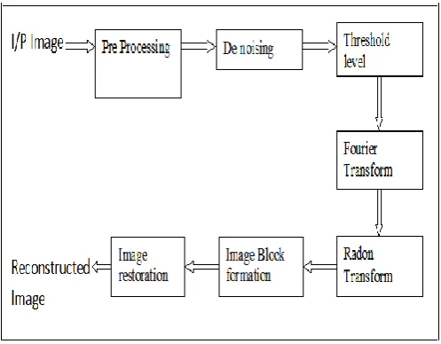
[image:4.595.312.561.501.695.2]The below block diagram shows the proposed approach for deconvolution algorithm.
Fig. 3.1 Overview of the proposed method
© 2016, IRJET | Impact Factor value: 4.45 | ISO 9001:2008 Certified Journal
| Page 1427
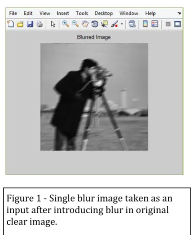
3.1.1. Input image:Proposed method based on the idea that it takes original image as an input then by adding motion blur by geometric function to it we get blurred image. This is done to understand the efficiency of proposed algorithm to remove blur from input image.
3.1.2. Pre-processing of an image:
One cannot process the image directly. Image may contain noise and other different ambiguities. It can be blurred or image details may get lost due to some reasons. For this image must be passed through the pre-processing stage. Pre-processing of an image also includes resizing of an image. The basic condition for any image processing algorithm is that images must be of same size for processing purpose. Different types of images are existing in data base. But in algorithm we necessity only one size of image. Hence in order to process out any image with respective algorithm we resize the input image in size (256*256). To see how many changes has been occurred in modified image we compute histogram of modified image. On this pre-processed image dual Fourier transform is implemented to calculate blur parameters.
3.1.3 Image De-noising
A digital image is a representation of a 2-dimensional image as a finite set of digital values, called picture elements or pixels. Noise not only degrades quality of image but also results in loss of important information in images. Therefore noise removal plays vital role in image enhancement and image restoration. It's necessary to have quality images without any noise to get accurate result. Noisy image may lead your algorithm towards in accurate result. Hence it becomes necessary to de-noise the image. Image processing researchers commonly assert that “median filtering is better than linear filtering for removing noise in the presence of edges.” Linear filtering is fundamental for signal processing, where often it is used to suppress noise while preserving slowly varying signal. In its simplest form, linear filtering consists of taking the average over a sliding window of fixed size. Indeed, linear filtering with fixed window size h “blurs out” the edges, causing a bias of order O(1) in a region of width h around edges. This blurring can be visually annoying and can dominate the mean-squared error.Median filtering taking the median over a sliding window of fixed size as a potential improvement on linear filtering in the “edgy” case. The main idea of the median filter is to
run through the signal entry by entry, replacing each entry with the median of neighbouring entries. The pattern of neighbours is called the "window", which slides, entry by entry, over the entire signal. For 1D signals, the most obvious window is just the first few preceding and following entries, whereas for 2D (or higher-dimensional) signals such as images, more complex window patterns are possible (such as "box" or "cross" patterns). Note that if the window has an odd number of entries, then the median is simple to define: it is just the middle value after all the entries in the window are sorted numerically. For an even number of entries, there is more than one possible median, see median for more details. The median is gotten by sorting all the values from low to high, and then taking the value in the centre.
3.1.4. Threshold level calculation:
After pre-processing and de-noising of an image it is essential to know that how much image has been blurred out. To find out level of blurriness in an image threshold calculation is done. Threshold calculation can be an indication of blurriness level in an image. Depending on threshold level calculation it will be decided up to how much extent we can decrease the block level size of a target image. MSE and PSNR are the algorithms generally implemented in image
processing in order to assess the performance of the codec of interest; they are closely linked to and borrowed from other contexts of signal processing.
Mean Square Error (MSE):
Let X and Y two arrays of size N x M, respectively representing the Y-channel frame of reference (i.e. the original copy) and Y-channel frame of the encoded/impaired copy. The mean square error between the two signals is thus defined as:
(3.1)
The more Y is similar to X, the more MSE is small. Obviously, the greatest similarity is achieved when MSE equal to 0.
Peak Signal to Noise Ratio (PSNR):
© 2016, IRJET | Impact Factor value: 4.45 | ISO 9001:2008 Certified Journal
| Page 1428
the PSNR is usually expressed in terms of the logarithmic decibel scale.
The mathematical demonstration of the PSNR is:
(3.2)
L reflects the range of values that a pixel can take.
3.1.5. Fourier transformation:
Fourier transformation is used to convert spatial domain in to frequency domain to eliminate & estimate blur component in an image. Fourier transform basically breaks down the image into the Fourier domain. This creates it much easier to method since you can now concentrate purely on discrete components of an image. Blur image is subjected to dual Fourier transform and radon transformation steps to obtain estimated values of blur length and blur angle respectively. In the problem of blind deconvolution, estimation of blur parameters is the most important step, as the quality and accuracy of estimation part greatly influences the quality of restoration. A single blurred image is analysed into frequency domain by taking its Fourier transform followed by radon transformation. Due to blur, this spectral representation reveals a typical sinc-like characteristics directed towards the direction of estimated angle. It also reveals the blur length information in terms of spectral width and image size. The two-dimensional Fast Fourier Transform (2D FFT) is an indispensable tool in many fields, including image processing, radar, optics and machine visualization. In image processing, the 2D Fourier Transform agrees one to understand the frequency spectrum of the data in both magnitudes and lets one imagine filtering processes more easily. The 2D Fourier Transform is only a Fourier Transform completed one dimension of the statistics, monitored by a Fourier Transform over the second dimension of the data. The 2D Inverse Fourier Transform is just the inverse Fourier Transform performed over both dimensions of the data.
Most of the energy in the Fourier domain is present in the center of the image, which corresponds to low frequency data in the picture domain. This links to the many slow changes in the picture. The stage of the FFTs is somewhat hard to understand visually and usually looks like noise. However, the phase holds a great deal of the information needed to reconstruct the image.
3.1.6. Image Block formation:
Threshold level indicates the level of Blurriness.
It is necessity of algorithm that for:-Large blurriness Block size must be decreased. Less blurriness Block size should be normal or increased.
As per above rules it is very clear that for high blurriness' user should perform micro-blocking of an image. Micro blocking is concerned with deep level processing of an image. With micro-blocking user is enabled to de-blur image at micro-level. Depending on blurriness level image can be converted in terms of blocks of different pixel sizes. By calculating PSNR (Peak signal to noise ratio) value extent of formation of blocks is decided. If PSNR value is less than 30 units then blocks are divided in 4*4 pixel size, if PSNR value is more than 30 units but less than 60 units then blocks are divided into 2*2 pixel size and if PSNR value is more than 60 then there is no need of block formation. This PSNR value is calculated by calculating first MSE (Mean square error) value. After block formation it will apply deconvolution to get original image
3.1.7. De-convolution
Deconvolution is a algorithm based mathematical operation used in image renovation to recover an object from an image that is degraded by blurring and noise. Deconvolution has its application in fields like digital signal processing and image processing.
There are two main methods of image deconvolution-
Standard Deviation (SD):
The standard deviation (SD) is a amount that is recycled to count the amount of difference or dispersion of a set of data values. A low SD indicates that the data points tend to be close to the mean (also called the expected value) of the set, while a high standard deviation indicates that the data points are spread out over a wider range of values. The good thing about the Standard Deviation is that ,we have a "standard" way of knowing what is normal, and what is extra-large or extra small. It is calculated as:
σ=
(3.3)
© 2016, IRJET | Impact Factor value: 4.45 | ISO 9001:2008 Certified Journal
| Page 1429
ability in calculating the unpredictability, it can be used in edge improving, as intensity level get changes at the edge of image by large value.
Variance:
Variance is the expectation of the squared deviation of a random variable from its mean. It is the square of the standard deviation. In order to get statistical behaviour of an image, we must know variance information. Mean value provides the influence of separate pixel strength for the whole image & variance is generally used to discover how each pixel differs from the adjacent pixel (or middle pixel) and is used in classify into different regions. It is the square of the standard deviation and calculated as:
σ2 =
(3.4)
Where X is the observed value, is the mean, n is total number of observed values. Variance filter can be utilized to determine edge position in image processing.
Blind deconvolution and Non blind deconvolution:
Blind deconvolution is a deconvolution technique that permits retrieval of the target scene from a single or set of blurry images in the attendance of a poorly strong-minded or indefinite point spread function (PSF). Even linear and non-linear deconvolution techniques use a recognized PSF. For blind deconvolution, the PSF is projected from the image or image set, permitting the deconvolution to be achieved. Blind deconvolution can be achieved iteratively, whereby each repetition recovers the approximation of the PSF and the scene, or non-iteratively, where one request of the algorithm, created on external information, extracts the PSF.
Wiener deconvolution:
In proposed algorithm deconvolution is performed in MATLAB software using ‘Wiener filter’. Wiener filter is one of the most widely used restoration techniques. Contrary to the inverse filtering this method also attempts to diminish noise although restoring the original signal. It performs an optimal balance between inverse filtering and noise smoothing in the mean square error sense. Wiener deconvolution is an application of the Wiener filter to the noise problems essential in deconvolution. It works in the frequency domain, trying to minimize the influence of deconvolved noise at frequencies which have a deprived
signal-to-noise ratio. The Wiener deconvolution technique takes extensive use in image deconvolution requests, as the frequency range of most visual images is fairly well behaved and may be estimated easily.
Standard application of wiener filter in MATLAB for deconvolution is illustrated as follow-
J=deconvwnr(I,PSF,NSR) deconvolved image I with the Wiener filter algorithm, recurring deblurred image J. Image I can be an N-dimensional array. PSF is the point-spread function through which I was convolved. NSR is the noise-to-signal power ratio.
4. RESULT AND DISCUSSION
4.1 Introduction
The experimental evaluation of proposed method is performed in MATLAB using Fourier algorithm and wienerde-convolution method are used to reconstruct original image. The proposed method analyses efficiency of algorithm to de-blur single image using Fourier transform and deconvolution based on statistical approach. The method is analysed in terms of histogram, MSE (mean square error), PSNR (peak signal to noise ratio), Blur parameters, Standard deviation and variance for measuring image quality. The deconvolution is based on wiener filter application
[image:7.595.332.524.491.727.2]4.2 Stepwise results of algorithm
© 2016, IRJET | Impact Factor value: 4.45 | ISO 9001:2008 Certified Journal
| Page 1430
[image:8.595.63.556.45.783.2]
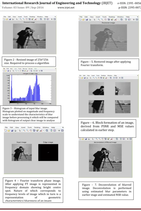
Figure 2 - Resized image of 256*256 size. Required to process a algorithm
Figure 3 – Histogram of input blur image. Histogram plotted on magnitude and frequency scale to understand the characteristics of blur image before processing it which will be compared with histogram of output clear image to analyse the changes occurred post deconvolution.
Figure 4 – Fourier transform phase image. After applying FT image is represented in frequency domain showing bright centre spot. Nature of which corresponds to frequency levels of image which in turn is a representation of geometric characteristics/sharpness of an image.
Figure – 5. Restored image after applying Fourier transform.
Figure – 6. Block formation of an image,
derived from PSNR and MSE values
calculated in earlier step.
© 2016, IRJET | Impact Factor value: 4.45 | ISO 9001:2008 Certified Journal
| Page 1431
Fig 4.1 Stepwise results of algorithm [image:9.595.76.522.73.777.2]
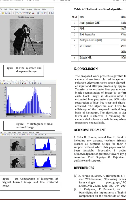
Table 4.1 Table of results of algorithm
5. CONCLUSION
The proposed work presents algorithm to remove camera shake from blurred image on MATLAB software. Algorithm takes single blurred image as an input and after pre-processing, applies Fourier Transform to estimate blur parameters. Further block segmentation of image is performed and each block image is de-convoluted by using estimated blur parameters and NSR value. Finally restoration of blur free clear and sharp image is achieved. The algorithm also helps to analyse efficiency of the proposed methodology on the basis of histogram. The algorithm is significantly faster and is effective in removing blur due to camera shake from a single image, when burst of images are not available.
ACKNOWLEDGMENT
I, Neha B. Humbe, would like to thank everyone, including my parents, teachers, friends and in essence all sentient beings for their help and support without which this paper would not have been possible. Especially, I dedicate my acknowledgment of gratitude toward my guide and co-author Prof. Supriya O. Rajankar for her guidance and support.
REFERENCES
[1] R. Fergus, B. Singh, A. Hertzmann, S. T. Roweis, and W.T.Freeman, “Removing camera shake from a single photograph,” ACM Trans. Graph., vol. 25, no. 3, pp. 787–794, 2006. [2] B. Carignan,J. F. Daneault, and C. Duval,“
Quantifying the imporatance of high frequency components on the amplitude of physiological Figure – 8. Final restored and
sharpened image.
Figure – 9. Histogram of final restored image.
© 2016, IRJET | Impact Factor value: 4.45 | ISO 9001:2008 Certified Journal
| Page 1432
tremor,” Experim. Brain Res., vol. 202, no.2, pp.299- 306
[3] J.-F. Cai, H. Ji, C. Liu, and Z. Shen, “Blind motion deblurring from a single image using sparse approximation,” in Proc. IEEE Conf. Comput. Vis. Pattern Recognit. (CVPR), Jun. 2009, pp. 104–111..
[4] L. Xu, S. Zheng, and J. Jia, “Unnatural L0 sparse representation for natural image deblurring,” in Proc. IEEE Conf. Comput. Vis. Pattern Recognit. (CVPR), Jun. 2013, pp. 1107–1114. [5] A.Rav-Acha and S. Peleg, “Two motion-blurred
images are better Than one,” Pattern RecognitLett., vol. 26, no. 3, pp. 311–317, 2005. [6] L. Yuan, J. Sun, L. Quan, and H.-Y. Shum, “Image deblurring with blurred/noisy image pairs,” ACM Trans. Graph., vol. 26, no. 3, 2007, Art. ID 1.
[7] HJiangyongDuan, GaofengMeng, Shiming Xiang, Chunhong Pan NLPR, Institution of Automation, Chinese Academy of Sciences, China “Removing out-of-focus blur from similar image pairs” ICASSP 2013
[8] Q. Shan, J. Jia, and A. Agarwala, “High-quality motion deblurring from a single image,” ACM Trans. Graph., vol. 27, no. 3, 2008, Art. ID 73. [9] D. G. Lowe, “Distinctive image features from
scale- Invariant keypoints,” Int. J. Comput. Vis., vol. 60, no. 2, pp. 91–110, 2004.
[10] J.-F. Cai, H. Ji, C. Liu, and Z. Shen, “Blind motion deblurring from a single image using sparse approximation,” in Proc. IEEE Conf. Comput. Vis. Pattern Recognit. (CVPR), Jun. 2009, pp. 104–111.
[11] S. H. Park and M. Levoy, “Gyro-based multi-image deconvolution for removing handshake blur,” in Proc. IEEE Conf. Comput. Vis. Pattern Recognit. (CVPR), Jun. 2014, pp. 3366–3373. [12] F. Gavant, L. Alacoque, A. Dupret, and D. David,
“A physiological camera shake model for image stabilization systems,” in Proc. IEEESensors, Oct. 2011, pp. 1461–1464.
[13] N. M. Law, C. D. Mackay, and J. E. Baldwin, “Lucky imaging: High angular resolution imaging in the visible from the ground,” Astron. Astrophys., vol. 446, no. 2, pp. 739–745, 2006. [14] V. Garrel, O. Guyon, and P. Baudoz, “A highly
efficient lucky imaging algorithm: Image synthesis based on Fourier amplitude selection,” Pub.Astron. Soc. Pacific, vol. 124, no. 918, pp. 861–867, 2012.
[15] D. L. Fried, “Probability of getting a lucky short-exposure image through turbulence,” J. Opt. Soc. Amer., vol. 68, no. 12, pp. 1651–1657, 1978.