SENTIMENT ANALYSIS USING REPRESENTATIVE TERMS A GROUPING APPROACH FOR BINARY CLASSIFICATION OF DOCUMENTS

(1)

ISSN: 1992-8645 www.jatit.org E-ISSN: 1817-3195

209

THE RESEARCH ON DATA STREAM CLUSTERING

ALGORITHM BASED ON ACTIVE GRID-DENSITY

1_{ZHONG ZHISHUI,}2_{WANG GANG}

1_{Department of Mathematics and Computer Science, Tongling University, Tongling, China}

ABSTRACT

The main work of this paper is to study and to achieve a time complexity of low and high precision of clustering data stream clustering algorithm. First is to analyze the data stream mining theory; to analyze and summarize several typical advantages and disadvantages of the traditional clustering algorithms, as well as the scope of application of clustering, which leads to data stream clustering algorithm and it’s elaborate; highlight a new data stream clustering algorithm: the data stream clustering algorithm is based on active mesh density. Firstly, the data space grid is divided into a grid structure formed by the small cube grid cell on the grounds, and then the data stream is mapped to this structure, the application of the concept is of density formation of the concept, and then feature vector to determine the density of the grid. The density attenuation of the dynamic is in the nature of the technology to capture data stream, and then extract the boundary point to remove it; introduce the concept of activity to determine the mesh density of active and inactive grid density to ignore the reserve of active grid density clustering, and in this article the algorithm CluStream algorithm for comparison. Finally, the algorithm is applied in this article to the network intrusion detection algorithm in the detection rate and false alarm rate analyzed to verify whether the algorithm is feasible or not.

Keywords: Data Stream, Clustering, Activity, Grid-Density

1. TRODUCTION

A continuous data stream, potentially unlimited, with high-speed mobility and other characteristics, which makes of the data stream mining algorithms, data can order one or more limited access. This feature of the data stream, the traditional mining method is difficult to meet their needs within a limited time. The result in depth study on the basis of the data stream clustering algorithm is given based on active mesh density data stream clustering algorithm (Data stream clustering algorithm is based on an active the grid density of AGD-Stream).

2. CLUSTREAM ALGORITHM BACKGROUND

Similarly, in the analysis of the data stream clustering algorithm, CluStream also played a huge role. Many stream clustering algorithm are CluStream clustering, thought them to the characteristics at the same time the Online / offline double the CluStream algorithm framework for data stream clustering algorithm to solve the contradiction between real-time requirements and quality of clustering in the data stream clustering problem through the framework of specific steps:

online micro-clustering process of the micro-cluster, offline clustering of macro macro-cluster process, and the framework structure of the pyramid. Micro-cluster summary information is stored up to use the macro clustering. CluStream algorithms involved in the pyramid time frame specific implementation process are as follows.

This framework snapshot saved in accordance with the data stream to reach the order, the order in accordance with the model of the pyramid is divided into different levels based on different information storage [3]:

1) Each layer can save up to

a

l

+

1

snapshot; (2) Part

i

layer a snapshot of

a

l , and

a

l divisible by the time of the snapshot corresponding to after the start of the data stream

a

, an integer multiple of time is the level to save a snapshot of the moment;

(3) Tier

i

of

a

or a divisible snapshot;

(4) Any known user-defined time window of

h

,

at least a snapshot of 2

h

in the distance the current time period.

(2)

210 a - as an integer, it determines the granularity of time

L - for the integer greater than 1, its size determines the arising

log

_a

T

- Pyramid maximum number of levels

This framework is to consider the storage requirements, taking into account the offline macro clustering in different time periods to restore the ability of the summary statistics [1-8].

Algorithm CluStream incremental clustering algorithm, STREAM algorithm is two less than any data stream arrives for processing, and can give any time to respond; faster by using the time frame of the pyramid according to treatment, can give different time granularity of the clustering results. However, CluStream algorithm has two shortcomings: (1) can only identify spherical clusters and clusters of arbitrary shape; (2) cannot handle the boundary points, the clustering accuracy is low. For each data point, the offline layer improved k-means algorithm is about all the initial data points for the kinds of division, and is able to identify the data points where a cluster is to calculate the data points with each distance between the centers. k-means algorithm the advantages is the ability to find the globular cluster, but the algorithm shortcomings - not the cluster of other shapes can be very efficient representation and mining, which determines the algorithm CluStream non-convex shape of the clusters relatively poor. In addition, because CluStream algorithm is based on k-means algorithm, which is determined by calculating the distance of data points and the center of its class affiliation, so it is not good at dealing with boundary points, largely affected the clustering effect, difficult to obtain accurate, high-quality clustering results, and the implementation of the algorithm is not efficient.

For the above CluStream algorithm cannot display any shape clustering, cannot effectively solve the boundary point two questions, this paper presents a data stream clustering algorithm based on active mesh density, which is able to identify the data of arbitrary shape and effectively address boundary issues. Firstly, the grid of data space is divided into a grid structure formed by a number of small cube grid cell, then the data stream is mapped to this structure, application of the concept of density is the formation of the concept of mesh density and density attenuation technology to capture the dynamic nature of the data stream, and then extract the boundary point to remove it; the

introduction of the concept of activity determines the mesh density of active and inactive grid density ignore retain active grid density of the final cluster . Experimental results show that, of AGD-Stream algorithms and CluStream algorithm compared to the arbitrary shape clusters that can be tapped to effectively solve the problem of boundary points, the time complexity of clustering accuracy have been improved.

3. AN IDEA OF THE DATA STREAM CLUSTERING ALGORITHM BASED ON ACTIVE MESH DENSITY

3.1The Basic Idea Of Algorithm

The basic idea is: the first grid of data space is divided into a grid structure formed by a number of small cube grid cell, then the data stream is mapped to this structure, the concept of the application of density mesh density concept, and then determine the density of the grid according to the feature vector. And use the density decay of the dynamic nature technology to capture the data stream.

3.2 Algorithm Description

AGD-Stream（X =

{

x1,L,xn

}

_,

t

_）

{

initialize（

grid

,

g

）; // Initialize the grid initialize（

grid

_

list

,

h

）; // Initialize the grid list

when there comes the data stream:

receive（X =

{

x1,L,xn

}

_,

t

_）_{; Receiving data set}

(X =

{

x1,L,xn

}

_,

t

_{) and record}

the mapping (

X

,

g

) ;// data is mapped to the division of good space-intensive grid

for（

i

=

1

;

i

<=

n

；

i

+ +

）// Identify the boundary points in a certain time interval period, and remove it from the grid

if (（

x

i_{is on the edge}_）_and_（

t

mod

gap

_{<> 0}

）)

for （

i

=

0

,

i

<=

n

,

i

+ +

）

switch （

x

i_）

{

(3)

211 case ‘not on the edge’:

judge the active of grid density;

update（V）;

break;

(// Determine whether the data points to meet another condition of the boundary pointscase ‘on the edge’:

inspect grid density ;

update（V）;

break;

}

else

update （

grid

）;// Otherwise, update the grid to meet the new distribution of the data stream

if （density（

g

））// If the density of the grid is active mesh density, and add it to the grid list

insert

g

into

hash

_

gridlist

;

if（

t

mod

gap

= =0）// The cluster density-based approach to intensive grid

cluster（

grid

）; }

3.3interval gap to Determine

The dynamic nature of the data stream can lead to the data density gradients over time. Some dense grid long time new data arrives, will lead to a very small amount of data in the grid, grid activity will reduce the attenuation of the transition grid or sparse grid. So we have to search for the density of each grid to a specified time interval, and then replace the original feature vector based on the results of the search, according to the dense nature of the grid to update the organizational structure of

each class. This time we require the value of

gap

should be appropriate. If value is too high, the test results cannot be timely performance of the fluctuations of the cluster; value too low will cause off-line processing be very complex, the calculated level rise, longer time, which cannot be consistent with the speed of data flow. Through the analysis mainly consider two aspects: (1) dense grid attenuation sparse grid, time-consuming the minimum (min); (2) sparse grid to update the minimum time-consuming for the dense grid. In order to guarantee sufficient time to detect the changes of the grid sparse, take (1), (2) the

minimum value as the value of

gap

, this article refers to the

gap

defined]:

Theorem 1 for any a dense network in terms of

the grid

g

, the dense grid failure become sparse grid with minimum time required.

0 log

l m C C λ

σ

= 

  _（₁_）

Theorem 2 for any sparse grid

g

in terms of sparse grid upgrade to the minimum of the dense grid time required

1

log

m l

N

C

N

C

λ

σ

=



−



−





_（₂_）

Based on the above two theorems, select

σ σ

0

,

1_,

the minimum value as the value of

gap

:

2 2

2

min

log

, log

log (max

,

)

l m

m l

l m

m l

c

N

c

gap

c

N

c

N

c

N

c









₋







=













−





















_

₋





=









−















₍₃₎

Where, N represents the number of grids.

3.4Handling Of Boundary Points

A grid density is less than

D

l_{, then there may be}

two reasons: (1) real data points by a small number of boundary points constitute a small grid, grid boundaries sparse network; that a few boundary constitute a point; (2) even if a lot of data in the grid, the grid density gradually decay over time, resulting in less data, this grid is called the decay sparse network grid; only the first few data points in a real situation of a small number of boundary points of the grid.

(4)

212 Definition 7 (density threshold) set the current

time

t

(

t

>

t

u_),

t

u_{the grid}

t

u_{last update data in}

time, then the density threshold is defined as

1 0

(1

)

( , )

(1

)

u

u t t

t t i l l u i

C

fun t t

N

λ

− + − =

−

=

−

∑

(4)

Theorem 3 density threshold

fun t t

( , )

u _{has the}

following properties:

（ 1 ）

t

1

≤ ≤

t

2

t

3 _， _Then

3 2

1 2 2 1 3 1 3

( , )

(

, )

( , )

t t

fun t t

fun t

t

fun t t

λ

−

+

=

（2）

t

1

≤

t

2_，_Then

fun t t

( , )

1

≥

fun t t

( , )

2 _，

（

t

>

t t

1

,

2_）

Proof: (1) from the known to have:

3 2

1 1

3 2 ₃ ₁ 3 2 2 1

3 2

3 2 3 1

1 2 2 1 3

0 0 0

1 3 0

( , ) ( , )

( , )

t t t t

t t

t t t t

t t i i i i

l l l l

i i i t t i

t t i l

i

fun t t fun t t

C C C C

N N N N

C

fun t t N

λ

λ λ λ λ

λ − − − − − + − − − + = = = − = − = + = + = + = =

∑

This completes the proof

Proof: (2) Order,

∆ = −

t

2

t

1

1 2 2 2

2 2

2

1

0 0 0 1

2 2

1 ( , )

( , ) ( , )

t t t t t t t t t t

i i i i

l l l l

i i i i t t

t t t i l

i t t

C C C C

fun t t

N N N N

C

fun t t fun t t N

λ λ λ λ

λ − − +∆ − − +∆ = = = = − + − +∆ = − + = = = + = + ≥

∑

This completes the proof

Here,

fun t t

( , )

u _{as in B-time test grid}

g

_{is a}

boundary the standard sparse grid. If

( , )

_u

D g t

<

fun t t

, then

g

is a boundary sparse grid. Can be seen that

fun t t

( , )

u _function

according to the formula can be used as a standard to distinguish the grid category, to determine what is "new" of the boundary point, which is the original stronghold of the majority. And can change over time to their adjustment, use the arrival time of the data points to analyze the size of the mesh density threshold.

If the moment of arrival of the nearest moment is longer, then the data points corresponding to the

density function value is smaller than

fun t t

( , )

u _;

the contrary, if just a new data point arrives, then the data points corresponding to the density function

value is bigger than

fun t t

( , )

u _{. This is not because}

it is the newly arrived data points to determine the number of less error as a boundary point to remove.

4. SIMULATION EXPERIMENTS AND RESULTS ANALYSIS

AGD-Stream algorithm testing laboratoriesand the performance Clustream algorithm, the experimental environment is: Intel Pentium 4 CPU 3.00GHz Memory 1.00GB, the operating system for Windows XP. Algorithm is written in MATLAB. The experimental data [8] use real data sets KDDCUP99 Network Intrusion Detection stream data set collected by the MIT Lincoln Laboratory, the dataset object is divided into five major categories and 41 properties.

In this study, [7] 34 are continuous attributes. And to make the = 3.5, = 0.9, with practice in other literature, this paper also used the 34 continuous attributes; the other is artificial data set [8]. Clustering effect of the detection algorithm on the non-convex shape of the data set, generated as shown in Figure 1, two-dimensional non-convex shape of the artificial data set, the data set contains three classes, two attributes. In this experiment, each data set standardized in order to unify the data set of dimension values in [0, l], and divided equally to all data in a different dimension, set up each dimension to divide the length indicated.

Analysis of the clustering process and the effect of the algorithm

(5)

213 In the experiment, each dimension by the length

of

len

= 0.05,

λ

= 0.99. The experimental results show that, AGD-Stream algorithm can effectively remove a large number of boundary points which can be better found three classes.

[image:5.612.331.503.127.461.2]

To illustrate the class of AGD-Stream algorithm can dynamically change and timely remove the boundary point. This article specifically dealt with in the next experimental data, making the data stream start to appear three types of data, and then to observe the clustering results for each time period. The experimental results show that, AGD-Stream algorithm can generate the data stream and disappear in a timely manner to reflect the latest clustering information, and can effectively remove the boundary points.

Figure 1 30 000 Data Points Randomly Distributed

Artificial data sets used in this experiment, the distribution of their data as shown in Figure 4. This article is in order to generate a certain order, a total of randomly generated 90 000 data points, including 20 000 boundary points, the data flow rate of 1000, where inflow l000 data, 80 per unit time. 30 per unit

time

t

1_{, 60 per unit time}

t

2_{, time}

t

3_{for 90 units of}

AGD-Stream algorithm in time

t

1 _clustering

evolution shown in Figure 5;

t

2_{moment of cluster}

evolution shown in Figure 6; clustering in the

t

3

time evolution shown in Figure 7.

Figure 5 indicates the class of AGD-Stream,

algorithms found in the beginning

t

1_{of time, while}

excluding the boundary points. Figure 6 show that

the class 1 at

t

2_{time gradually disappeared, the}

algorithm to find all the boundary points and delete at the same time to find a class 2, Figure 7 shows

that

t

3_{at the moment, the data flow all over the}

clustering results of the moment.

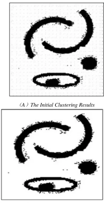
（A）The Initial Clustering Results

（B）The Final Clustering Results Figure 2 Representation Of Clustering Results

The class to identify the pieces of the chart and clear of AGD-Stream algorithm can be concentrated accurate data points, such as the above classes disappear and the process, but also ample evidence that the algorithm can effectively detect and remove the boundary points

5. SUMMARY

[image:5.612.116.273.292.450.2]

(6)

214 concept of activity to find the active grid density, the final cluster. The algorithm can be clusters of arbitrary shape and effectively deal with border issues. Reference time interval is a cluster period of time, reducing the computational load. Compared with CluStream algorithm, experiments show that of AGD-Stream, the algorithm's time complexity and accuracy of clustering have been improved.

ACKNOWLEDGEMENT

The paper is financed by Anhui University Provincial Natural Science Research Project(KJ2011B184),the Nature Science Foundation of Anhui Province(090416247) ,and

Collage Outstanding Young Talent

Fund(2009SQRZ175).

REFERENCES

[1] Han J, Kamber M. Data mining: concepts and technique. 2nd. Beijing China Machine Press, 2007: 306-307P

[2] Wang Xianpeng grid-based MST data stream clustering algorithm. Harbin Engineering University, a master's degree thesis .2009:4-35 [3]Yang Ning, jie, Wang Yue, Chen Yu, Zheng Jiao

Ling [7] based on the density of states tilt distribution of the data stream clustering algorithm. Journal of Software, 2009,21 (5) :1-11

[4] Jae Woo Lee, Nam Hun Park, Won Suk Lee. Efficiently tracing clusters over high-dimensional on-line data streams. Data and Knowledge Engineering. 2009, 68 (3) :362-379P

[5] Li W, Xuan H, PHILIP S Y. Density-based clustering of data streams at multiple resolutions. ACM Transactions on Knowledge Discovery from Data (TKDD). 2009,3 (3) :14-42P

[6] Zhu Wei Heng, seal, Xieyi Huang, arbitrary shape based on the data flow clustering algorithm, Journal of Software .2006,17 (3): 379-387

[7] Xue L, Qiu B. Density-reachable based clustering algorithm for multi-density. Computer Engineering. 2009, 35 (17) :66-68P

[8] Zhao L., Mao Y.X, GOBO: a Sub-Ontology API for Gene Ontology, IEIT Journal of Adaptive & Dynamic Computing, 2011(1), Jan 2011, pp:29-32.

DOI=10.5813/www.ieit-web.org/IJADC/2011.1 .5

[9] Zhu X.D, Block Correlations Directed Multi-copies Data Layout Technology, IEIT Journal of Adaptive & Dynamic Computing,

2011(1), Jan 2011, pp:33-38.