http://dx.doi.org/10.4236/jsip.2014.51004
Object Tracking Using a New Level Set Model
Nagi H. Al-Ashwal, Abdulmajid F. Al-Junaid
Electrecal Engineering Department, Ibb University, Ibb, Yemen. Email: [email protected]
Received November 18th, 2013; revised December 18th, 2013; accepted December 25th, 2013
Copyright © 2014 Nagi H. Al-Ashwal, Abdulmajid F. Al-Junaid. This is an open access article distributed under the Creative Com-mons Attribution License, which permits unrestricted use, distribution, and reproduction in any medium, provided the original work is properly cited. In accordance of the Creative Commons Attribution License all Copyrights © 2014 are reserved for SCIRP and the owner of the intellectual property Nagi H. Al-Ashwal, Abdulmajid F. Al-Junaid. All Copyright © 2014 are guarded by law and by SCIRP as a guardian.
ABSTRACT
This paper proposes a novel implementation of the level set method that achieves real-time level-set-based object tracking. In the proposed algorithm, the evolution of the curve is realized by simple operations such as switching values of the level set functions and there is no need to solve any partial differential equations (PDEs). The object contour could change due to the change in the location, orientation or due to the changeable nature of the object shape itself. Knowing the contour, the average color value for the pixels within the contour could be found. The estimated object color and contour in one frame are the bases for locating the object in the consecutive one. The color is used to segment the object pixels and the estimated contour is used to initialize the deformation process. Thus, the algorithm works in a closed cycle in which the color is used to segment the object pixels to get the ob-ject contour and the contour is used to get the typical-color of the obob-ject. With our fast algorithm, a real-time system has been implemented on a standard PC. Results from standard test sequences and our real time system are presented.
KEYWORDS
Object Tracking; Deformable Model; Level Set Method; HSI Color Space
1. Introduction
Tracking is the problem of generating an inference about the motion of an object given a sequence of images. Good solutions to this problem have a variety of applica-tions areas including surveillance [1-7], human-computer interfaces [3,4], and medical imaging [8,9].
Deformable models have been used in tracking tasks [8] and [10-12]. Deformable model is appealing for object tracking because the object in the image sequence can vary from frame to frame due to a change in the view point, the motion of the object, or its nonrigid nature. The principal challenges for object tracking using deformable models are to develop accurate deformable model of im- age variability and to design computationally efficient tracking algorithms which use this model. Also paramet- ric deformable models have some difficulties in handling topological changes such as the merging and splitting of object regions. For these reasons, the level set me- thod [13,14] is a more powerful technique. But the high
computational cost of the level set method has limited its popularity in real-time scenarios.
their evolution equation they defined two lists of neighboring pixels Lin and Loutof the contour Γ( )t . Their level set is evolved by switching the neighboring pixels between the two lists Lin and Lout.
In this paper, we propose a novel approach to tracking using the level set methods. Our approach is based on that the implicitly represented curves can be moved by changing the sign of values of the level set function in-side and outin-side the curve. Our approach requires simple addition operation and then changes the sign of some values inside or outside the curve to achieve the tracking. Our method does not contain any functional energy, so it does not need to solve any partial differential equations (PDEs), thus reducing the computation dramatically compared with other techniques proposed before. The proposed tracking technique tries to trace both contour and color variations in order to locate the object in the consecutive frames. With our approach, real-time level- set-based video tracking can be achieved by using a con- ventional PC.
The rest of the paper is organized as follows. In Sec-tion 2 we give a brief review of the level set methods. Section 3 presents the new level set technique for track-ing. In Section 4 the proposed technique for object tracking is described. The experimental results are pre-sented in the Section 5. The paper is concluded in Sec-tion 6.
2. Level Set Methods
The main idea behind the level set formulation is to represent an interface Γ
( )
t bounding a possibly multi- ply connected region in Rn by a Lipschitz continuous function φ, changing sign at the interface, i.e.( )
( )
( )
( )
( )
( )
, 0, if is inside , , 0, if is at , , 0, if is outside .
x t x t
x t x t
x t x t
φ φ φ
> Γ
= Γ
< Γ
(1)
In numerical implementations, often regularity is im-posed on φ to prevent the level set function of being too steep or flat near the interface. This is normally done by requiring φ to be the signed distance function to the interface
( )
(
( )
)
( )
( )
( )
( )
(
( )
)
( )
, , , if is inside ,
, 0, if is at ,
, , , if is outside ,
x t d t x x t
x t x t
x t d t x x t
φ φ φ
= Γ Γ
= Γ
= − Γ Γ
(2)
where d
(
Γ( )
t ,x)
denotes Euclidian distance between x and Γ( )
t . We emphasize that requiring (2) is a techni-cality to prevent instabilities in numerical implementa-tions.The interface Γ
( )
t is implicitly moved according to the nonlinear PDE( )
. 0,t
φ ν φ φ
∂ + ∇ =
∂ (3)
where ν φ
( )
is a given velocity field. This vector field can depend on geometry, position, time and internal or external physics. Usually only the velocity normal to the interface νN is needed, and φ is then moved accord-ing to the modified equation( )
0.N t
φ ν φ φ
∂ + ∇ =
∂ (4)
3. Tracking Level Set Model
In this paper, we use a region-based level set model for the object tracking. The tracking process is depending on the quality of the matching between the object contour and the interface of the level set function, Γ
( )
t . The tracked object is segmented then the tracking process is started.The used level set function, φ is be given by:
( )
( )
( )
( )
( )
( )
( )
1 if , is inside , , 2 if , is outside ,
0 if , is in ,
r c t
r c r c t
r c t
φ
Γ
= − Γ
Γ
(5)
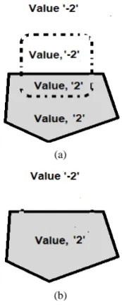
where (r,c) are the row and column coordinates of the current point. From (5) we can conclude that φ contains two regions, inside region with value “+1” and outside region with value “−2”, see Figure 1.
Our method does not need to solve any PDE, so regu-larity is not important. Therefore φ is not required to be a distance function. The tracked object is segmented and given the value “1”, the value “0” is reserved for the background, see Figure 2.
Deformation
The deformation process is started by adding both the segmented image, I, see Figure 2, and the current level set function φn, see Figure 1. The result is put in a new image called ψ ,
.
n I
ψ = +φ (6)
Every intersection between the object region, and level set regions has a unique value in the resultant image, ψ. It is clear that any point in ψ will take its value based on the following:
( )
r c, z z,{
2, 1,1, 2 .}
ψ = = − − (7)
The number of points carrying any value, z, in ψ gives information about the amount of overlap between the level set function and the object, we have four states, see Figure 3:
Figure 1. Proposed level set model, ϕ.
Figure 2. Segmented image model,I(r,c).
Figure 3. The resultant image after the addition, ψ(r,c). of φ,represents the area in which the object misses the interior region of φ.
2) The number of occurrence of the value “2” repre-sents the area in which the object hits the interior region of φ.
3) The number of occurrence of the value “1”, results from the addition of the background and the interior region of φ, represents the area in which the interior region of φ misses the object.
4) The number of occurrence of the value “−2”, re-sults from addition of the background and exterior region of φ,represents the area in which the exterior region of
φ hits the background.
The next step is the deformation process which is done by simply changing some values in the resultant image, ψ. The values are changed to force the interface contour,
( )t
Γ , to catch the object’s boundary. By considering the object-mask arrangement shown in Figure 3, we can observe that to force Γ( )t to catch the object the values of φ should be changed based on the following rules, see Figure 4:
1) The pixels of values “−2” and“2” remain without change,
2) the pixels of value “1” is regarded as outside region so it should be changed to the value “−2”,
3) the pixels of value “−1” is regarded as inside region
(a)
(b)
Figure 4. Deformation process, (a) changing values in ψ to catch the object, (b) the new level set function, ϕ after catching the object.
so it should be changed to the value “2”. The above steps can be achieved by:
( )
( )
( )
( )
1
2 if , 1, , 2 if , 1,
, otherwise.
n
r c
r c r c
r c ψ
φ ψ
ψ
+
= −
= − =
(8)
4) Finally, to get the level set model in (5) the pixels of the exterior region are changed to the value “−1”,
( )
( )
( )
( )
( )
1 1 if , is inside , ,
2 if , is outside .
n r c t
r c
r c t
φ + = Γ
− Γ
(9)
4. Proposed System
In this section our algorithm for object tracking is de-scribed. Before the start of tracking process there are two necessary steps. The first step, Display, is to select the object for tracking. Second step, Initialization, is carried out to locate the object contour.
4.1. Display
The captured images are previewed and the initial level set function, ϕ, is created by hand and given values as shown in Figure 1. The process is done by putting the interface Γ
( )
t over the object needed to be tracked, seeFigure 5 in the experimental result section. 4.2. Initialization
[image:3.595.132.216.299.393.2]Display and Initialization
Frame 1 Frame 60
Frame 150 Frame 200
[image:4.595.62.285.90.486.2]Frame 250 Frame 300
Figure 5. Example 1 of the tracking of an object.
tation we could easily segment the object by assum- ing that the changes of the object hue or saturation are much smaller than the expected changes in the intensity. Thus the object is a blob in the image with limited va- riation in hue and saturation and slightly larger variation in the intensity. The object segmentation is performed in two steps: 1) get the typical-color of the object, see
Algorithm 1, and 2) use the typical-color to threshold the current frame to extract the object, see Algorithm 2, the resultant image, I, is binary image with object and background values as shown in Figure 2.
Now we have φ and I so (6) can be used to find the new image, ψ . The new φn+1, which catches the object,is then found by (7) and (8).
4.3. Tracking-Target
The tracking is a sequence of operations; the first step is to use the level set function, φ, from the previous frame,
Algorithm 1. Get the typical color of the object.
Get Hsi Thresholds
Find the average of values of HAV, SAV, IAV of pixels
in the region which encircled by a contour
Inputs Image, I, Leve set function, ϕ
Outputs the average values HAV, SAV, IAV
Steps
Initialize HAV = 0; SAV = 0; IAV = 0; No Of Pixels = 0;
for I = 0 toImage Rowsdo
begin
for j = 0 to Image Columnsdo
begin
if image(i,j) is inside the region which encircled by modelthen
begin
HAV = HAV + image(i,j, HUE) SAV = SAV + image(i,j, SATURATION)
IAV = IAV + image(i,j, INTENSITY) No Of Pixels = No Of Pixels + 1
end end end HAV = HAV/No Of Pixels,
SAV = SAV/No Of Pixel, IAV = IAV/No Of Pixels
Algorithm 2. Extract the object.
Extract Object
Extract the object by set most of its pixels to value “1” and most of other pixels in the image to value “0”
Inputs HSI Image, HAV, SAV, IAV, tH, tS, tI/* tH is
tolerance of plane H*/
Outputs
Segmented binary Image BW(r,c) in which most of the object pixels are “1” and most of the
background pixels are “0”
Steps
Hupper = HAV + tH, Hlower= HAV – tH Supper = SAV +tS, Slower = SAV – tS
Iupper = IAV +tI, Ilower = IAV – tI
for i = 0 toImage Rowsdo
begin
for j = 0 to Image Columnsdo
begin
( )
( )
(
)
( )
( )
lower upper
lower upper
lower upper
1 , ,
and( , , )
,
and( , , )
0 Otherwise
if H I r c H H S I r c S S BW r c
I I r c I I
≤ ≤
≤ ≤
=
≤ ≤
end end
in order to get the typical-color in the current frame. The second step is to use this color for object segmentation, i.e. getting the image I. Finally we use I and φ to deform the model towards a better fit using the steps in Section 3.A. By this the interface of the level set will move to catch the moved target.
4.4. Advantages and Disadvantages
algorithms may not work properly when the objects abruptly change their motion from one frame to the next [20,21]. Such situations can be due to collisions or sharp turns. Also the algorithms that detect motion in a sequence of frames by extracting tokens such as edges, corners, interest points, etc. [22,23] mistake objects when there is a change in their 2-dimensional shape [24,25]. The solution of the above problems is to use high frame rate. By maintaining the interframe time small, we main-tain both shape and color variation to minimum. High frame rate requires a high speed tracking algorithm to segment and track the object in the small interframe time.
The proposed method does not contain any PDE and the tracking process is done by simple addition and change values operations, see (6) and (8). Thus, the speed of deformation is the strongest point in the pro-posed system. It is capable of tracking objects at 30 frames/sec on regular PC (CORE 2 Duo). Each of the frames is 480 × 640 RGB 24-bit pixels. This speed keeps the color position and shape variation in the interframe time small. Consequently the reliability of the tracking process increases.
The most important limitation of the proposed system is that it loses track of the object when the object is par-tially occluded by similar color object. In this case the deformation algorithm tends to combine both similar color objects within a single contour. As one of the ob-ject moves away from the other the algorithm will follow both objects. Also, the algorithm gives poor results if there is no color difference or intensity contrast between the object and the background as with all tracking algo-rithms.
5. Experimental Results
In this section two examples are given to demonstrate the system capability for real time tracking. In all experi-ments we used CORE 2 Duo Laptop with 2.2 GHz speed and 4 GB memory.
5.1. Example 1
The used video is taken using a webcam at 30 frames per second. The sequence consists of frames each of (480 × 640 pixels). As shown in Figure 5, frame 0 shows the object (blue paper) with the initial model being place on it. The initial contour is determined manually using the mouse. In the initialization the deformation process is used to get the contour of the object. As can be clearly shown in some subsequent frames in Figure 5, the pro-posed system is able to continuously track the object real time. The motion of the contour is due to the change of the location of the object.
5.2. Example 2
The proposed system is applied to track an object in a
video downloaded from the internet. The downloaded video has 30 frames per second each is 480×640 pixels.
Figure 6 shows the tracking results of the object. The object color and contour are used for tracking. Despite the motion and shape changes of the object, the deform-able model reasonably delineates the contour of the ob-ject throughout the whole sequence.
6. Conclusion
This paper introduced a new tracking algorithm that is fast enough to track an object in real time. The used defi-nition of an object is any connected area in the captured frame which has a consistent feature. Although arbitrary complex feature could be used, the one selected is the HSI representation of color which practically fits a wide range of applications. A deformable model which de-pends on the level set methods has been pursued because
Display and Initialization
Frame 1 Frame 100
Frame 200 Frame 250
[image:5.595.310.534.306.720.2]Frame 300 Frame 400
of its speed and simplicity. The deformation requires only two-image addition to obtain the contour of the tar-get object. Using this algorithm, a real time system was constructed using a standard CORE 2 Duo Laptop. Many experiments are made on real videos with frame rate of 30 frames/sec. The result showed that the proposed tech-nique can track an object in real time.
REFERENCES
[1] H. Meyerhoff, F. Papenmeier and M. Huff, “Object- Based Integration of Motion Information during Attentive Tracking,” Perception, Vol. 42, No. 1, 2013, pp. 119-121. http://dx.doi.org/10.1068/p7273
[2] A. Feldman, M. Hybinette, T. Balch and R. Cavallaro, “The Multi-ICP Tracker: An Online Algorithm for Track- ing Multiple Interacting Targets,” Journal of Field Robo- tics, Vol. 29, No. 2, 2012, pp. 258-276.
http://dx.doi.org/10.1002/rob.21402
[3] S. B. Gokturk, C. Tomasi, B. Girod and J.-Y. Bouguet, “Model-Based Face Tracking for View-Independent Fa- cial Expression Recognition,” 5th IEEE International Conference on Automatic Face and Gesture Recognition, Washington, 21-21 May 2002, pp. 287-293.
[4] M. Wang, Y. Iwai and M. Yachida, “Expression Recogni- tion from Time-Sequential Facial Images by Use of Ex- pression Change Model,” 3rd IEEE International Con-
ference on Automatic Face and Gesture Recognition, Nara, 14-16 April 1998, pp. 324-329.
http://dx.doi.org/10.1109/AFGR.1998.670969
[5] O. Javed and M. Shah, “Tracking and Object Classifica-tion for Automated Surveillance,” The 7th European Conference on Computer Vision (ECCV 2002), Copen- hagen, 2002, pp. 343-357.
[6] R. Howarth and H. Buxton, “Visual Surveillance Moni- toring and Watching,” Proceedings of European Confer-
ence on Computer Vision, Vol. 2, 1996, pp. 321-334.
[7] T. Frank, M. Haag, H. Kollnig and H.-H. Nagel, “Track-ing of Occluded Vehicles in Traffic Scenes,” Proceedings of European Conference on Computer Vision, Vol. 2, 1996, pp. 485-494.
[8] N. Ray and S. T. Acton, “Active Contours for Cell Tracking,” 5th IEEE Southwest Symposium on Image Analysis and Interpretation, Sante Fe, 7-9 April 2002, pp. 274-278.
[9] E. Bardinet, L. Cohen and N. Ayache, “Tracking Medical 3D Data with a Deformable Parametric Model,” Pro- ceedings of European Conference on Computer Vision, Vol. 1, 1996, pp. 317-328.
[10] G. Unal, H. Krim and A. Yezzi, “Active Polygon for Object Tracking,” 1st International Symposium on 3D Data Processing Visualization and Transmission (3DPVT’ 02), 2002, p. 696.
[11] Y. Q. Chen, T. Huang and Y. Rui, “Mode-Based Multi- Hypothesis Head Tracking Using Parametric Contours,” 5th IEEE International Conference on Automatic Face
and Gesture Recognition, Washington, 20-21 May 2002, pp. 112-117.
[12] Y. Zhong, A. K. Jain and M.-P. Dubuisson-Jolly, “Object Tracking Using Deformable Templates,” IEEE Transac- tions on Pattern Analysis and Machine Intelligence, Vol. 22, No. 5, 2000, pp. 544-549.
http://dx.doi.org/10.1109/34.857008
[13] S. Osher and N. Paragios, “Geometric Level Set Methods in Imaging, Vision and Graphics,” Springer Verlag, 2003.
[14] J. Sethian, “Level Set Methods and Fast Marching Meth- ods: Evolving Interfaces in Computational Geometry, Fluid Mechanisms, Computer Vision, and Material Sci-ence,” Cambridge University Press, 1999.
[15] M. Kass, A. Witkin and D. Terzopoulos, “Snakes: Active Contour Models,” International Journal of Computer Vi-sion, Vol. 1, No. 4, 1988, pp. 321-331.
http://dx.doi.org/10.1007/BF00133570
[16] S. Besson, M. Barlaud and G. Aubert, “Detection and Tracking of Moving Objects Using a New Level Set Based Method,” Proceedings of ICPR, Vol. 3, 2000, pp. 1100-1105.
[17] D. Adalsteinsson and J. Sethian, “A Fast Level Set Meth- od for Propagating Interfaces,” Journal of Computational Physics, Vol. 118, 1995, pp. 269-277.
[18] N. Paragios and R. Deriche, “Geodesic Active Contours and Level Sets for the Detection and Tracking of Moving Objects,” IEEE Transactions on Pattern Analysis and Machine Intelligence, Vol. 22, 2000, pp. 266-280. [19] Y. G. Shi and W. C. Karl, “Real-Time Tracking Using
Level Sets,” Proceedings of IEEE Conference on Com-puter Vision Pattern Recognition (CVPR ‘05), Vol. 2, 2005, pp. 34-41.
[20] H. Shariat and K. E. Price, “Motion Estimation with more than Two Frames,” IEEE Transaction on Pattern Analy- sis and Machine Intelligence, Vol. 12, No. 5, 1990, pp. 417-432. http://dx.doi.org/10.1109/34.55102
[21] B. K. P. Horn and B. Schunck, “Determining Optical Flow,” Artificial Intelligence, Vol. 17, No. 1-3, 1981, pp. 185-203.
http://dx.doi.org/10.1016/0004-3702(81)90024-2
[22] X. Zhuang, T. S. Huang, N. Ahuja and R. M. Haralick, “A Simplified Linear Optic Flow-Motion Algorithm,”
Computer Vision, Graphics and Image Processing, Vol. 42, No. 3, 1988, pp. 334-344.
http://dx.doi.org/10.1016/S0734-189X(88)80043-4 [23] L. S. Davis, Z. Wu and H. Sun, “Contour-Based Motion
Estimation,” Computer Vision, Graphics and Image Processing, 1982, pp. 313-326.
[24] R. Bergevin and M. D. Levine, “Extraction of Line Drawing Features for Object Recognition,” Pattern Rec-ognition, Vol. 25, No. 3, 1992, pp. 319-334.
http://dx.doi.org/10.1016/0031-3203(92)90113-W [25] C. Cédras and M. Shah, “Motion-Based Recognition: A