A report on using parallel MATLAB for solutions to stochastic optimal control problems

Munich Personal RePEc Archive

A report on using parallel MATLAB for

solutions to stochastic optimal control

problems

Azzato, Jeffrey D. and Krawczyk, Jacek B.

Victoria University of Wellington

12 August 2008

A REPORT ON USING PARALLEL MATLABR _{FOR SOLUTIONS TO}

STOCHASTIC OPTIMAL CONTROL PROBLEMS

JEFFREY D. AZZATO & JACEK B. KRAWCZYK

Abstract.

Parallel MATLAB

is a recent MathWorks

prod-uct enabling the use of parallel computing methods on

mul-ticore personal computers.

SOCSol

_{is the generic name of a}

suite of MATLAB

_{routines that can be used to obtain}

opti-mal solutions to continuous-time stochastic optiopti-mal control

problems. In this report, we compare the performance of a

new version of

SOCSol

_{utilising parallel MATLAB}

_{with that}

of another version not using parallel computing methods.

2008 Working Paper

School of Economics and Finance

JELClassification: C63 (Computational Techniques), C87 (Economic Software). AMSCategories: 93E25 (Computational methods in stochastic optimal control). Authors’Keywords: Computational economics, Approximating Markov decision chains.

This report documents 2008 research into Computational Economics Methods

directed by Jacek B. Krawczyk and supported by URF GMS Grant 32665

Correspondence should be addressed to:

Jacek B. Krawczyk. Faculty of Commerce and Administration, Victoria University of Wellington, P.O. Box 600, Wellington, New Zealand. Fax: +64-4-4635014 Email:

Contents

Introduction 1

1. The Test Problems 2

1.1. The First Test Problem 2

1.2. The Second Test Problem 2

2. Measuring Computation Times 3

3. Comparison of Solution Routines 4

3.1. The First Test Problem 4

3.2. The Second Test Problem 5

4. Summary 6

Appendix A. SOCSol4L_{Commands for the First Test Problem 6}

A.1. Delta Function File 6

A.2. Instantaneous Cost Function File 7

A.3. Terminal State Function File 7

A.4. Solution Syntax 7

Appendix B. Parallel SOCSol_{Commands for the First Test Problem 7}

B.1. Function Files 8

B.2. Solution Syntax 8

Appendix C. SOCSol4L_{Commands for the Second Test Problem 8}

C.1. Delta Function File 8

C.2. Instantaneous Cost Function File 8

C.3. Terminal State Function File 8

C.4. Solution Syntax 8

Appendix D. Parallel SOCSol_{Commands for the Second Test Problem 9}

D.1. Function Files 9

D.2. Solution Syntax 9

Appendix E. Tables of Computation Times 9

Introduction

Performing independent calculations in parallel should make it possible to dramat-ically reduce overall computation times for certain types of problem, such as those solvable by dynamic programming. One class of problems solvable by dynamic pro-gramming are the stochastic optimal control (soc) problems. These are frequently

either analytically unsolvable, or sufficiently complicated for analytical solutions to be impractical. Consequently, good numerical methods for solving socproblems are

desirable.

A method for approximating a solution to a given continuous-time socproblem was

developed in [KW97] and subsequently improved in [Kra01]. The method works by discretising the problem in both state and time, forming an equivalent Markov chain and then solving this Markov chain by backward induction. While elementary, this approach has the advantages of generality and providing feedback (as opposed to open-loop) solutions. A disadvantage of this approach is that it is subject to the “curse of dimensionality” when the state space is effectively multidimensional (i.e., when d > 1 —see Section 1): halving the discretisation steps of all state variables

simultaneously increases computation time by a factor of 2d.1 So implementing this approach for high-dimensionalsocproblems rapidly becomes computationally costly.

However, parallel computing may provide a means of fighting this phenomenon. In backward induction, computing the optimal return for a given state and time only requires knowledge of optimal returns at the next time. The state-independence of this calculation means that it can be performed in parallel across several different states simultaneously. So increasing the number of parallel workers by a factor of 2d when halving all state discretisation steps should leave overall computation time relatively unchanged. Of course, it is not always realistic to exponentially increase computing resources. Nonetheless, the growing prevalence of multicore processors and small computing grids makes this approach increasingly attractive.

A suite of MATLABR2 _{routines implementing the method described in [Kra01] was}

developed under the name SOCSol4L_{. The use of this suite is described in [AK06].} With the introduction of extensive parallel computing support in MATLABR_{, a new}

suite of MATLABR _{routines implementing the same method using parallel computing}

methods is being developed under the name Parallel SOCSol_{. The use of this new} suite is described in [AK08].

This article compares the computation times of the two suites of routines for a pair of deterministic test problems. Each test problem was solved with each suite for various discretisations on each of two different computers. This should help to quantify the potential of applying parallel computing methods in this area of research.

1_{In particular, ifd=1, halving the state discretisation step doubles computation time—an outcome}

not shared by all approaches based on dynamic programming.

1. TheTestProblems

The method employed by the SOCSol4L _and Parallel SOCSol _{suites of MATLAB}R routines deals with finite-horizon, free terminal statesoc problems having the form

min

u J(u,x0) = E

Z T

0 f x(t),u(t),t

dt+h x(T)

x(0) =x₀

(1)

subject to

dx=g x(t),u(t),t

dt+b x(t),u(t),t dW

(2)

where T > 0 is the length of the optimisation horizon, x: [0,T] → X ⊆ Rd _{is state}

evolution, u: [0,T] → U ⊆ Rc _{is control and W is a standard Wiener process in}

which precisely N 6 _{d components are not constantly zero (so the state space has}

dimension d, the control has dimensioncand N state variables are affected by noise). The method also allows for constraints on the control and state variables (both local and mixed).

In order to provide a basis for comparison, we solved two deterministic (i.e., W ≡0) test problems of this form using both SOCSol4L _and Parallel SOCSol_{. These are} formulated as described below.

1.1. The First Test Problem. The first test problem is an elementary linear-quadratic optimal control problem having a one-dimensional state space. It involves the min-imisation of

J1

u,1 2

:=

Z 1

0

u(t)2_+x(t)2

2 dt+

x(1)2

2 (3)

with respect to u, subject to

dx =u(t)dt, and (4)

x(0) = 1 2. (5)

1.2. The Second Test Problem. The second test problem is similar to the first, but involves a two-dimensional state space in which the control u now affects the first state variable x₁ only indirectly through the second state variable x2. It involves the

minimisation of J2 u, 1 0 := Z 1 0

u(t)2+x2(t)2

2 dt+

x1(1)2

2 (6)

with respect to u, subject to

dx =

x₂(t)

u(t)

dt, and (7)

2. MeasuringComputationTimes

Computation times were obtained for the test problems of Section 1 by treating the relevant solution routine (of either SOCSol4L _or Parallel SOCSol_{) as a “black box,”} simply timing how long it took to run. This approach determines alterations in com-putation times as they would be experienced by a user. It would also be possible to directly measure alterations in computation times for those subroutines that have been “parallelised.” While this might quickly quantify how much improvement could be obtained under a parallel implementation, it is unrealistic, as most programs involve some fixed overhead (e.g., for initilisation and saving output).

The SOCSol4L_{solution routine is structured as follows.}

{ I n i t i a l i s e p a r a m e t e r s }

f o r { e a c h s t a t e }

{ Compute t e r m i n a l o p t i m a l r e t u r n }

end;

f o r { e a c h s t a g e }

f o r { e a c h s t a t e }

{ Compute o p t i m a l r e t u r n , o p t i m a l c o n t r o l and p o s s i b l y L a g r a n g e m u l t i p l i e r s }

end;

end;

{ S a v e r e s u l t s }

The Parallel SOCSol_{solution routine modifies this basic structure as follows.}

{ I n i t i a l i s e p a r a m e t e r s } { Open a MATLAB p o o l }

p a r f o r { e a c h s t a t e }

{ Compute t e r m i n a l o p t i m a l r e t u r n }

end;

{ S t o r e t e r m i n a l o p t i m a l r e t u r n }

f o r { e a c h s t a g e }

p a r f o r { e a c h s t a t e }

{ Compute o p t i m a l r e t u r n (OR) , o p t i m a l c o n t r o l s ( OCs ) and p o s s i b l y L a g r a n g e m u l t i p l i e r s ( LMs ) }

end;

{ S t o r e OR, OCs and p o s s i b l y LMs }

end;

Here, each parfor loop executes in parallel. So if there are two MATLABR

work-ers in the pool, the loop can (in principle) execute in half of the time taken by the corresponding for loop. However, this decrease in computation time is balanced by increases in fixed overhead due to

1. the opening and closing of the pool of MATLABR _{workers, and}

2. the need to use temporary variables within the parfor loops, the content of which is subsequently transferred to the arrays of interest.

As a consequence, we expect that Parallel SOCSol_{will take longer than}SOCSol4L_to solve “small” socproblems, but may be nearly twice as fast for “large”socproblems

when using two MATLABR _{workers. Here, a “large” soc problem is one in which}

the relevant solution routine (of either SOCSol4L _or Parallel SOCSol_{) is run over a} discrete state grid containing a sufficiently large number of points. Such grids can arise from either

1. high-dimensional state spaces (i.e., large numbers of state variables), or 2. fine discretisation of the state variable(s).

3. Comparison ofSolutionRoutines

Here we compare the times taken by the solution routines of SOCSol4L_and Parallel SOCSol _{to solve the test problems defined in Section1. Each test problem was solved} with each solution routine for various discretisations on each of two different com-puter systems. The full results are tabulated in AppendixE.

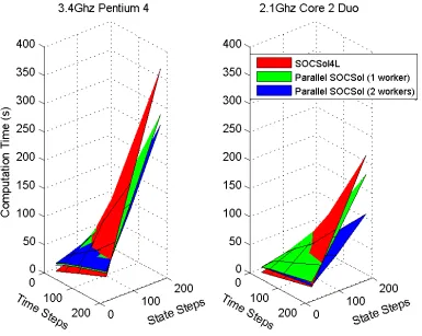
3.1. The First Test Problem. The times achieved for the first test problem are dis-played in Figure1. Several unsurprising trends are immediately clear from this figure, namely:

• Finer state discretisation (i.e., more state steps) increases computation time. • Finer time discretisation (i.e., more time steps) increases computation time. • The 2.1GHz CoreTM 2 Duo computer system is faster than the 3.4GHz

PentiumR _{4 computer system.}

Two other trends are also clear from Figure 1. The first of these is that SOCSol4L outperforms Parallel SOCSol _{when state-time discretisation is sufficiently coarse,} and vice-versa when state-time discretisation is sufficiently fine. This is consistent with the heuristic analysis given in Section 2. Examination of the values tabulated in Appendix E suggests that the time improvements introduced by the parallel code in Parallel SOCSol_{outweigh the additional fixed overheads imposed when the discrete} state-time grid used has of the order of 10000 points or more.

The second interesting trend apparent in Figure 1 is that for “large” choices of the state-time grid (i.e., 10000 points or more), using two workers in Parallel SOCSol yields much greater relative time reductions with the CoreTM 2 Duo computer system than with the PentiumR _{4 system. For example, if both state and time steps are set}

to 0.005 (yielding a state-time grid having 36000 > 10000 points), using two

work-ers instead of one yields only an additional 5% time reduction when operating on

the PentiumR _{4 system (79% vs. 74%). However, using two workers instead of one}

yields an additional 32% time reduction when operating on the CoreTM2 Duo system (85% vs. 53%) — a marked decrease. This supports the hypothesis that computation time improvements obtained through parallel MATLABR _{are likely to be greater with}

newer generation CPUs.

Figure 1: Computation times for the first test problem.

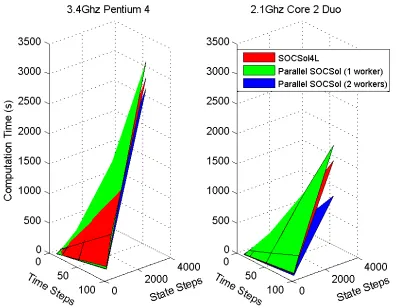
Figure 2: Computation times for the second test problem.

4. Summary

The use of parfor loops in MATLABR _{implementations of the soc problem solution}

method described in [Kra01] both introduces additional fixed overhead and the po-tential for reductions in loop running times. The experimental results presented here suggest that reductions in loop running times are likely to outweigh the additional fixed overhead for sufficiently large problems when at least two MATLABR _workers

are used in parallel. The results are also consistent with the hypothesis that reduc-tions in overall computation time are more likely to be achieved when using newer generation CPUs.

AppendixA. SOCSol4L_Commands for theFirstTestProblem

The SOCSol4L_{commands used to obtain results for the first test problem are detailed} below. This section should be read in conjunction with [AK06].

A.1. Delta Function File. This.m_{file defines the problem’s dynamics g x}(_t),_u(_t),_t. It is called delta.m_{and is written as follows.}

f u n c t i o n v = d e l t a ( u , x , t ) v = u ;

A.2. Instantaneous Cost Function File. This.m_{file gives the instantaneous cost} func-tion f x(t),u(t),t

. It is calledcost.m _{and is written as follows.}

f u n c t i o n v = c o s t ( u , x , t ) v = 0 . 5∗u^2 + 0 . 5∗x ^ 2 ;

A.3. Terminal State Function File. This .m _{file gives the terminal state function}

h x(T)

. It is calledterm.m _{and is written as follows.}

f u n c t i o n v = term ( x ) v = 0 . 5∗x ^ 2 ;

A.4. Solution Syntax. It is easiest to write a MATLABR _{script to set the SOCSol4L}

parameters and call theSOCSol _{solution routine. An example of such a script is given} below for state and time discretisation steps each equal to 0.02. The tic; and toc; commands time how long theSOCSol _{solution routine takes to execute.}

S t a t e L B = −0.2; StateUB = 0 . 7 ;

Options = { ’ TolFun ’ ’ 1e−12 ’ } ; I n i t i a l C o n t r o l V a l u e = −0.5; A = [ ] ;

b = [ ] ; Aeq = [ ] ; beq = [ ] ;

ControlLB = −I n f; ControlUB = I n f;

U s e r C o n s t r a i n t F u n c t i o n F i l e = [ ] ;

S t a t e S t e p = 0 . 0 2 ; % T h i s v a r i e s .

TimeStep = ones ( 1 , 5 0 ) / 5 0 ; % T h i s v a r i e s .

t i c ;

SOCSol ( ’ d e l t a ’ , ’ c o s t ’ , ’ term ’ , StateLB , StateUB , S t a t e S t e p , TimeStep , ’ SOCSol4L_TestProb1_02_02 ’ , Options ,

I n i t i a l C o n t r o l V a l u e , A, b , Aeq , beq , ControlLB , ControlUB , U s e r C o n s t r a i n t F u n c t i o n F i l e ) ;

t o c;

AppendixB. Parallel SOCSol _Commands for the FirstTestProblem

B.1. Function Files. The delta function file, instantaneous cost function file and ter-minal state function file are defined as per Appendices A.1, A.2and A.3 respectively.

B.2. Solution Syntax. A MATLABR _{script is written exactly as shown in}

Appen-dix A.4, except that the Options vector is altered to either Options = { ’ P o o l S i z e ’ ’ 1 ’ ’ TolFun ’ ’ 1e−12 ’ } ;

or

Options = { ’ P o o l S i z e ’ ’ 2 ’ ’ TolFun ’ ’ 1e−12 ’ } ;

as appropriate, and the name for the output files is altered sensibly, perhaps to ’ParallelSOCSol_PoolSize2_TestProb1_02_02’.

AppendixC. SOCSol4L_Commands for the SecondTestProblem

The SOCSol4L_{commands used to obtain results for the first test problem are detailed} below. This section should be read in conjunction with [AK06].

C.1. Delta Function File. This .m_{file is called}delta.m _{and is written as follows.}

f u n c t i o n v = d e l t a ( u , x , t ) v = [ x ( 2 ) , u ] ;

C.2. Instantaneous Cost Function File. This.m _{file is called}cost.m _{and is written as} follows.

f u n c t i o n v = c o s t ( u , x , t ) v = 0 . 5∗u^2 + 0 . 5∗x ( 2 ) ^ 2 ;

C.3. Terminal State Function File. This .m _{file is called} term.m _{and is written as} follows.

f u n c t i o n v = term ( x ) v = 0 . 5∗x ( 1 ) ^ 2 ;

C.4. Solution Syntax. An example of a MATLABR _{script setting the SOCSol4L}

pa-rameters and calling the solution routineSOCSol_{for state and time discretisation steps} each equal to 0.01.

S t a t e L B = [ 0 . 5 , −0 . 5 ] ; StateUB = [ 1 . 5 , 0 . 5 ] ;

Options = { ’ TolFun ’ ’ 1e−12 ’ } ; I n i t i a l C o n t r o l V a l u e = −0.5; A = [ ] ;

b = [ ] ; Aeq = [ ] ; beq = [ ] ;

ControlLB = −I n f; ControlUB = I n f;

U s e r C o n s t r a i n t F u n c t i o n F i l e = [ ] ;

S t a t e S t e p = [ 0 . 0 1 , 0 . 0 1 ] ; % T h i s v a r i e s .

TimeStep = ones ( 1 , 1 0 0 ) / 1 0 0 ; % T h i s v a r i e s .

t i c ;

SOCSol ( ’ d e l t a ’ , ’ c o s t ’ , ’ term ’ , StateLB , StateUB , S t a t e S t e p , TimeStep , ’ SOCSol4L_TestProb2_01_01_01 ’ , Options ,

I n i t i a l C o n t r o l V a l u e , A, b , Aeq , beq , ControlLB , ControlUB , U s e r C o n s t r a i n t F u n c t i o n F i l e ) ;

t o c;

AppendixD. Parallel SOCSol _Commands for theSecondTestProblem

The Parallel SOCSol _{commands used to obtain results for the first test problem are} detailed below. This section should be read in conjunction with [AK08].

D.1. Function Files. The delta function file, instantaneous cost function file and ter-minal state function file are defined as per Appendices C.1, C.2and C.3respectively.

D.2. Solution Syntax. A MATLABR _{script is written exactly as shown in}

Appen-dix C.4, except that the Options vector is altered to either Options = { ’ P o o l S i z e ’ ’ 1 ’ ’ TolFun ’ ’ 1e−12 ’ } ;

or

Options = { ’ P o o l S i z e ’ ’ 2 ’ ’ TolFun ’ ’ 1e−12 ’ } ;

as appropriate, and the name for the output files is altered sensibly, perhaps to ’ParallelSOCSol_PoolSize2_TestProb2_01_01_01’.

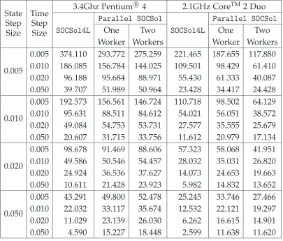
AppendixE. Tables ofComputationTimes

PentiumR _{4 CPU, 2Gb of RAM and a Windows}R _{XP Home Edition operating system.}

The second had a 2.1GHz CoreTM 2 Duo CPU, 2Gb of RAM and a WindowsR _XP

Professional operating system. In each case, the computation times were measured with only those background processes activating on system startup operating in the background.

It should be noted that each computation time quoted is not an average over several executions of the problem whose computation time was to be measured. This should be taken into account when making inferences using these values.

State Step Size

Time Step

Size

3.4Ghz PentiumR _{4 2.1GHz Core}TM _{2 Duo}

Parallel SOCSol Parallel SOCSol

SOCSol4L _{One Two} SOCSol4L _{One Two}

Worker Workers Worker Workers

0.005

0.005 374.110 293.772 275.259 221.465 187.655 117.880 0.010 186.085 156.784 144.025 109.501 98.429 61.410 0.020 96.188 95.684 88.971 55.430 61.333 40.087 0.050 39.707 51.989 50.964 23.428 34.417 24.428

0.010

0.005 192.573 156.561 146.724 110.718 98.502 64.129 0.010 95.631 88.511 84.612 54.021 56.051 38.572 0.020 49.084 54.753 53.731 27.577 35.555 25.679 0.050 20.607 31.715 33.756 11.612 20.979 17.134

0.020

0.005 98.678 91.469 88.606 57.323 58.068 41.951 0.010 49.586 50.546 54.457 28.032 35.031 26.820 0.020 24.924 36.536 37.627 14.073 24.653 19.663 0.050 10.611 21.428 23.923 5.982 14.832 13.652

0.050

0.005 43.291 49.800 52.478 25.245 33.746 27.466 0.010 22.032 33.117 35.674 12.532 22.121 19.297 0.020 11.029 23.139 26.030 6.262 16.615 14.901 0.050 4.590 15.227 18.448 2.599 11.638 11.620

Table 1: Computation times (in seconds) for the first test problem.

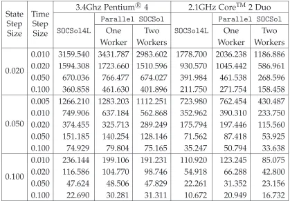
State Step Size

Time Step Size

3.4Ghz PentiumR _{4 2.1GHz Core}TM _{2 Duo}

Parallel SOCSol Parallel SOCSol

SOCSol4L _{One Two} SOCSol4L _{One Two}

Worker Workers Worker Workers

0.020

0.010 3159.540 3431.787 2983.602 1778.700 2036.238 1186.886 0.020 1594.308 1723.660 1510.596 930.570 1045.442 586.961 0.050 670.036 766.477 674.027 391.984 461.538 268.596 0.100 360.858 461.630 401.896 211.750 271.754 158.458

0.050

0.005 1266.210 1283.203 1112.251 723.980 762.454 430.487 0.010 749.906 637.184 562.868 352.962 390.310 233.750 0.020 374.455 325.713 289.249 175.794 197.446 115.560 0.050 151.185 140.254 128.146 71.562 87.418 53.925 0.100 74.929 79.804 75.165 35.247 50.794 33.638

0.100

0.010 236.144 199.106 191.231 110.920 123.245 85.075 0.020 116.586 104.770 98.746 54.918 66.288 42.800 0.050 47.624 48.506 47.829 22.261 31.352 23.156 0.100 22.690 30.281 31.311 10.672 20.949 16.732

Table 2: Computation times (in seconds) for the second test problem.

References

[AK06] Jeffrey D. Azzato and Jacek B. Krawczyk. SOCSol4L: An improved MATLABR _{package for}

approximating the solution to a continuous-time stochastic optimal control problem. Working paper, School of Ecnomics and Finance, Victoria University of Wellington, Dec 2006.

[AK08] Jeffrey D. Azzato and Jacek B. Krawczyk. Parallel SOCSol: A parallel MATLABR _{package for}

approximating the solution to a continuous-time stochastic optimal control problem. Working paper, School of Ecnomics and Finance, Victoria University of Wellington, Jul 2008.

[Kra01] Jacek B. Krawczyk. A Markovian approximated solution to a portfolio management prob-lem. ITEM., 1(1), 2001. Available at http://www.item.woiz.polsl.pl/issue/journal1.htm

on 22/04/2008.

[KW97] Jacek B. Krawczyk and Alistor Windsor. An approximated solution to continuous-time sto-chastic optimal control problems through Markov decision chains. Technical Report 9d-bis, School of Economics and Finance, Victoria University of Wellington, 1997. Available at

http://ideas.repec.org/p/wpa/wuwpco/9710001.htmlon 31/07/2008.