Tau Collocation Approximation Approach for Solving First and Second Order Ordinary Differential Equations

(1)

http://dx.doi.org/10.4236/jamp.2016.42045

Tau-Collocation Approximation Approach

for Solving First and Second Order

Ordinary Differential Equations

James E. Mamadu

1

, Ignatius N. Njoseh

2

1_{Department of Mathematics, University of Ilorin, Ilorin, Nigeria}

2_{Department of Mathematics and Computer Science, Delta State University, Abraka, Nigeria}

Received 25 January 2016; accepted 23 February 2016; published 26 February 2016

This work is licensed under the Creative Commons Attribution International License (CC BY). http://creativecommons.org/licenses/by/4.0/

Abstract

This paper presents Tau-collocation approximation approach for solving first and second orders ordinary differential equations. We use the method in the stimulation of numerical techniques for the approximate solution of linear initial value problems (IVP) in first and second order ordinary differential equations. The resulting numerical evidences show the method is adequate and effec-tive.

Keywords

Ordinary Differential Equation (ODE), Initial Value Problem (IVP), Canonical Polynomial, Collocation

1. Introduction

(2)

provide approximate polynomial solution for linear ordinary differential equation with polynomial coefficient. The method takes advantage of the special properties of Chebychev polynomials. The main idea is to obtain an approximate solution of a given problem by solving an approximate problem. To further enhance the desired simplicity Lanczos introduced the systematic use of the canonical polynomials in the Tau method. The difficul-ties presented by the construction of such polynomials limited its application to first order ODE with the poly-nomial coefficient. The said difficulties were resolved by [2] when he proposed the generation of these canoni-cal polynomials recursively. The beauty of the result of Ortiz is that the elements of canonicanoni-cal polynomials se-quences by means of a simple recursive relation which is self starting and explicit. There are many literature developed concerning the Tau/Tau-collocation approximation method (see ([3]-[8])).

In this paper, we apply the Tau-collocation approximation method for the solution of linear initial value prob-lems of the first and second order ODE in its differential and canonical form. We perform some numerical sti-mulation on some selected problems and compare the performance/effectiveness of the method with the analytic solutions given.

2. The Tau Method

Lanczos [1] approximated a solution y x

( )

of the differential

( )

_{( )}

_{, 0} ₁

m

r r r o

P x y f x x

=

= ≤ ≤

∑

(1)

where P x_r

( )

, f x

( )

are polynomials. ( )r

( )

y x denotes the rth order derivative of y x

( )

with respect to x

and y( )0

( )

x taken simply as y x

( )

by a polynomial

( )

,

n r

r o

y x a x n

=

∑

< ∞ (2)

and determines the coefficient a rr, =0 1

( )

n of (2) such that yn

( )

x satisfies (1) perturbed by a term(s), which

are calculated as part of the process. That is, y_n

( )

x satisfies

( )

_{( )}

_.

m

r

r n

r o

P x y f x H x

=

= +

∑

(3)

Then

( )

1 *

1, 0 1

m s

n m s r n m r

r o

H x T x

+ −

+ − − + + =

=

_∑

≤ ≤ (4)

where m is the order of the differential equation, s is the number of over-determination,

( )

1 1

r= m+s, are the parameters to be determined, and

( )

* 1

0

2

Cos Cos

r r k

r k

k

x a b

T x r C x

b a

−

=

  − − 

= _ _ __≡

−

 

 

∑

(5)

is the rth degree shifted Chebychev polynomial valid in the interval

[ ]

a b, (assuming (1) is defined in this in-terval).

The free parameters in Equation (4) and the coefficient ar, r∈0 1

( )

n in (2) are obtained by equating the

values of x in (3) together with (1) to zero.

2.1. Description of the Differential Form

Considering the mth order linear differential Equation ([1] [2])

( )

(

)

_: m

( )

( )r

_{( )}

_,

r r o

L y x P x y f x

=

_∑

= (6)

( )

_{( )}

( ) 1

0 1 1

0 , 0 , , m 0 _m ,

(3)

with y(x) as the exact solution in a≤ ≤x b a, < ∞,b < ∞.

We seek an approximate solution of the differential solution by the Tau method using the nth degree poly-nomial function

( )

,

m

r

n r

r o

y x P x x n

=

_∑

< ∞ (7)

which satisfies the perturbed problem

( )

(

)

_: m

( )

( )r

_{( )}

r n

r o

L y x P x y f x H x

=

_∑

= + (8)

We equate the corresponding coefficient of x in (8) and using the initial conditions

( )

_{( )}

( ) 1

0 1 1

0 , 0 , , m 0 _m ,

y =

α

y′ =

α

 y − =

α

₋

We then solve the system of equation by Gaussian elimination method.

2.2. Collocation Approach to the Tau Method

The Lanczos Tau method in [4] is an economization process for a function that is implicitly defined by differen-tial equation. Let us assume an approximation of the power series expansion u x

( )

as

( )

n

( )

r

n r

r o

u x a x x

=

∑

(9)

Consider an approximation to the residual R x_n

( )

as

( )

*

( )

*

( )

*

( )

1

1 2 m 1

n n n n m

R x = T x + T− x + + T− + x (10)

Then by the Tau method, if

( )

(

)

( )

L u x = f x (11)

we have

( )

(

)

( )

*

( )

2

* 1

*

1 m 1

n n n n m

L u x = f x +R x = f x + T x + T₋ x ++ T_{− +} x (12)

where L is a linear differential operator of order n.

We collocate (12) at xk =kh k, =1 1

( )

N, where

1

b a

h n

− =

+ to have

( )

(

)

( )

1

( )

2

( )

* * *

1 1

k k n k k n k n k m n m k

L u x = f x +R x = f x + T x + T− x ++ T− + x (13)

The parameter 1, 2,,m may be eliminated leaving the unknown coefficient a k_k, =0 1

( )

n with

(

n+1

)

linear equations which can be solved by Gaussian elimination.

3. Error Estimation

Let us in this section consider and obtain the error estimator for the approximate solution of (1) and (9). Let

( )

n n

E =u x −u x be the error function of u_n

( )

x to u x

( )

, where u x

( )

is the exact solution of (1) and (9).

Therefore u_n

( )

x satisfies the perturbed problems:

( )

(

)

(

( )

)

( )

_{( )}

_{[ ]}

0

: ( ) , , , , ,

m

r

n r n n

r

L u x P x u x f x H x x a b a b n

=

∑

= + ∈ < ∞ < ∞ < ∞ (14)

and

( )

(

)

( )

0

: m

r

n r n

r

L u x a x f x H x

=

(4)

where Hn is uniquely defined as in (4).

To obtain the perturbation term H_n

( )

x , we substitute the computed solution u_n

( )

x such that

( )

(

)

( ) ( )

(

)

( )

_{( )}

0

: m

r

n r n n

r

L u x P x u x f x H x

=

_∑

− =

and

( )

(

)

( )

0

: m

r

n r n

r

L u x a x f x H x

=

_∑

− =

We then proceed to find an approximate En N,

( )

x to the error function En

( )

x in the same manner as we

did for the solution of (1) and (9).

Thus, the error function, En, satisfy the problem

( )

0

: m

r

n r n n

r

L E P x E f x H x

=

_∑

− = − (16)

and

( )

0

: 0

m r

n r

r

L E a x f x

=

∑

− = (17)

which satisfies the conditions prescribed.

4. Illustrative Examples

In this section, two initial value problems are considered to show the efficiency of the method. Example 1

Consider linear initial value problem in second order ordinary differential equation

( ) ( )

( )

0 1,

( )

1 03

u x u x

u u

′′

 + =



 ₌ _′ ₌

 (18) We solve [4] for n=2 using; (i) The Tau method; and (ii) Tau-collocation method.

The analytic solution is

( )

Cos Sin

(

Cos1 3

)

. Sin1

x

u x = x− −

By the Tau method we obtain the linear differential operator as

2

d 1 d L

x

 

≡_ + _

  (19) The associated canonical polynomials are obtained as follows:

2

d 1 d

r r

Lx x

x

 

=_ + _

  (20)

(

1

)

2

( )

r

r r

Lx =r r− LQ− x +LQ x

(

)

( )

1 1

2 1 r

r r

L− ⋅Lx =L− ⋅ L r r_ − Q₋ x +Q x _

(

1

)

2

( )

r

r r

x r r Q− x Q x

⇒ = − +

( )

(

1

)

2

( )

r

r r

Q x x r r Q₋ x

⇒ = − −

The canonical polynomials, Q x rr

( )

, ≥0, obtained here can easily be obtained from [3] where the

(5)

( )

0 1, 1

Q x = Q x =x and Q₂

( )

x =x2– 2

These polynomials are substituted into Equation (12) to give

( )

1

( )

* 2

* 1

n n n

Lu x = T x + T− x (21)

Using Equation (5),

( )

( ) 1 ( )1

_{( )}

1 2

0 0

n n

n

n r r

r r

Lu x C x C x x

− −

= =

=

∑

+

∑

( )

_{( )}

1 ( )1

_{( )}

1 2

0 0

n n

n r r r r

r r

Lu x C LQ x C LQ x

− −

= =

=

_∑

+

_∑

( )

_{( )}

1 ( )

_{( )}

1

1 2

0 0

n n

n r r r r

r r

u x C Q x C Q x

− −

= =

=

∑

+

∑

(22)

Since 𝑛𝑛= 2

( )

2 ( )2

_{( )}

1 ( )1

_{( )}

2 1 2

0 0

n

r r r r

r r

u x C Q x C − Q x

= =

=

_∑

+

_∑

Now,

( )

0 1, 1 2 1

T x = T x = x− and T₂

( )

x =8x2−8x+1

( )

(

( )2

_{( )}

( )2

_{( )}

( )2

_{( )}

)

(

( )1

_{( )}

( )1

_{( )}

)

2 1 0 0 1 1 2 2 2 0 0 1 1

u x = C Q x +C Q x +C Q x + C Q x +C Q x

( )

(

2

)

(

)

2 11 8 8 2 2 1 2

u x x x x

⇒ = − + − + − + (23)

Using initial conditions on Equation (23) and simplifying further we get the approximate solution as

( )

2

46 16

1

15 15

u x = + x− x .

Considering the Tau-collocation method we have: Let

( )

2

( )

2

0

r r r

u x a x x

=

∑

(24)

( )

2

2 0 1 2

u x =a +a x+a x

( )

2 1 2 2

u′ x = +a a x

( )

2 2 2

u′′ x = a

Substituting into (13) we have,

( )

2 * *

2 0 1 2 1 2 2 1

2a +a +a x+a x = T x + T x (25)

(

)

(

)

(

)

2 2

2 0 1 2 1 2

2a +a +a x+a x = 1 8− x+8 x −2 + − +1 2x

Now collocating at , , 1, 2, 3 1

k

b a

x kh h k

n

−

= = =

+ and using the initial conditions, we obtain the approximate solution as

( )

2

46 16

1

15 15

u x = + x− x

Example2

(6)

( ) (

1

) ( ) ( )

0,

( )

0 1

Ly x = +x y x′ +y x = y = (26)

The exact solution is

( )

1 1

y x x

= +

For the given IVP, we can deduce that m=1 and s=0. The differential formulation is as follows:

Let

( )

n r

r o

y x a x

=

∑

(27)

Taking n=5

( )

1 *

( )

5 1

m s

m s r n m r r o

Ly x T x

+ −

+ − − + + =

=

∑

( )

0 *

5 1 5

r o

Ly x T

= ⇒ =

_∑

where ( ) 5 5 * 5 r r r o

T C x

=

∑

(28)

hence

(

) ( )

( )

*

( )

5 5 1 5

1+x y′ x +y x = T x (29)

but

( )

5 ( ) 5

5 1

r r r o

Ly x C x

=

∑

Using (28) and (30) in (29) we obtain,

(

)

5 5 5 ( )

5 1

1

1 r r r r r r

r o r o r o

x ra x− ra x C x

= = =

+

∑

+

∑

=

∑

(31)

Expanding and equating coefficients of powers of x, the resulting linear equations together with the equations obtained using the initial conditions is written in the form,

Ax=b

where ( ) ( ) ( ) ( ) ( ) ( ) 5 0 5 1 5 2 5 3 5 4 5 5

1 1 0 0 0 0

0 2 2 0 0 0

0 0 3 3 0 0

0 0 0 4 4 0

0 0 0 0 5 5

0 0 0 0 0 0

1 0 0 0 0 0 0

C C C C C C                                 

(

)

T

0, 1, 2, 3, 4, 5,1

x= a a a a a a ,

(

)

T

0, 0, 0, 0, 0, 0,1

b=

(7)

( )5 ( )5 ( )5 ( )5 ( )5 ( )5

0 1, 1 50, 2 400, 3 1120, 4 1280 and 5 512.

C = − C = C = − C = C = − C =

Using these values in the matrix and solving by Gaussian elimination method, we have,

0 1 2 3 4 5 1

2339 1132 932 512 128 3

1, , , , , ,

2342 1171 1171 1171 1171 2342

a = a = − a = a = − a = a = − =

The approximate solution is:

( )

(

2 3 4 5

)

5

1

2342 2339 2264 1864 1024 256

2342

y x = − x+ x − x + x − x

Discussion of Results

The results obtained above show that the Tau-collocation method is appropriate for the solution of linear initial value problems of first and second kind ordinary differential equations. From the tables (Table 1and Table 2) of results presented above, we observe that the approximate solution considered at grid points, n=2 and

5

n= , for examples 1 and 2 converges to the analytic solution with maximum absolute errors of 10−3 and 10−5

respectively. We obtain satisfactory results because of the excellent convergence rate of the Tau-colloca-

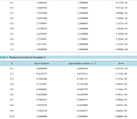
Table 1.Numerical results for example 1.

X Exact Solution Approximate solution, n = 2 Error

0.1 1.2868265 1.2960000 9.1735e−03

0.2 1.5607954 1.5706667 9.8712e−03

0.3 1.8191694 1.8240000 4.8306e−03

0.4 2.0593669 2.0560000 3.3669e−03

0.5 2.2789879 2.2666667 1.2321e−02

0.6 2.4758379 2.4560000 1.9838e−02

0.7 2.6479502 2.6240000 2.3950e−02

0.8 2.7936051 2.7706667 2.2938e−02

0.9 2.9113471 2.8960000 1.5347e−02

[image:7.595.89.538.327.716.2]

1.0 3.0000000 3.0000000 0.0000e+00

Table 2.Numerical results for Example 2.

X Exact Solution Approximate solution, n = 2 Error

0.1 0.9090909 0.9090418 4.19133e−05

0.2 0.8333333 0.8332214 1.1195e−04

0.3 0.7692308 0.7691735 5.7276e−05

0.4 0.7142857 0.7143198 3.4081e−05

0.5 0.6666667 0.6667378 7.1164e−05

0.6 0.6250000 0.6250298 2.9821e−05

0.7 0.5882353 0.5881915 4.3800e−05

0.8 0.5555556 0.5554809 7.4633e−05

0.9 1.5263158 0.5265873 2.8445e−05

(8)

tion approximation method, which is very close to the minimax polynomial which minimizes the maximum er-ror in approximation. Thus, the approximate solution will match the analytic solution as n increases.

5. Conclusions

This paper has considered Tau-collocation approximation approach for solving particular first and second order ordinary differential equations. The method offers several advantages which include, among others:

1) It takes advantages of the special properties of Chebychev polynomials which can be easily generated re-cursively;

2) Elements of canonical polynomials sequences by means of a simple re-cursive relation which is self start-ing and explicit; and

3) It can easily be programmed for experimentation.

Tau-Collocation method can be extended to higher order ordinary differential equations and stochastic diffe-rential equations. It can also be used to solve integro-diffediffe-rential and stochastic integro-diffediffe-rential equations.

References

[1] Lanczos, C. (1956) Applied Analysis. Prentice-Hall, Engle-Wood Cliffs, New Jersey. [2] Ortiz, E.L. (1969) The Tau Method. SIAM Journal on Numerical Analysis, 6, 480-492.

http://dx.doi.org/10.1137/0706044

[3] Yisa, B.M. and Adeniyi, R.B. (2012) A Generalized Formulation for Canonical Polynomials for M-Th Order Non Over-Determined Ordinary Differential Equations. Internal Journal of Engineering Research and Technology.

www.ijert.org

[4] Coleman, J.P. (1974) Lanczos Tau Method. IMA Journal of Applied Mathematics, 7, 85-97.

[5] El-Daou, M.K., Ortiz, E.L. and Samara, H. (1993) A Unified Approach to the Tau Method and Chebychev Series Ex-pansion Technique. Computer and Mathematics with Applications, 25, 73-82.

http://dx.doi.org/10.1016/0898-1221(93)90145-L

[6] Ortiz, E.L. (1975) Step by Step Tau-Method—Part 1. Computer and Mathematics with Applications, 1, 381-392.

http://dx.doi.org/10.1016/0898-1221(75)90040-1

[7] Khajah, H. (1999) Tau-Method Approximation of a Generalized Epstein-Hubbel Elliptic Type Integral. Computer and Mathematics, 68, 1615-1621. http://dx.doi.org/10.1090/S0025-5718-99-01128-X