Changes in the dynamical behavior of nonlinear systems induced by noise

CHANGES IN THE DYNAMICAL BEHAVIOR

OF NONLINEAR SYSTEMS INDUCED

BY NOISE

P.S. LANDA!, P.V.E. McCLINTOCK"

!Department of Physics, LomonosovMoscow State University, 119899 Moscow, Russia

"Department of Physics, Lancaster University, Lancaster LA1 4YB, UK

*Corresponding author.

E-mail address:[email protected] (P.V.E. McClintock)

Changes in the dynamical behavior of nonlinear systems

induced by noise

Polina S. Landa

!

, P.V.E. McClintock

"

,

*

!Department of Physics, LomonosovMoscow State University, 119899 Moscow, Russia "Department of Physics, Lancaster University, Lancaster LA1 4YB, UK

Received April 1999; editor: I. Procaccia

Contents

1. Introduction 4

2. Fluctuational transitions of nonlinear systems

from one stable steady state to another 4

2.1. Elements of the theory of#uctuational

transitions 4

2.2. Applications of the theory of#uctuational transitions to the problems of intermittency 12 3. Noise-induced transport of Brownian particles

(stochastic ratchets) 19

3.1. Noise-induced transport of light Brownian particles in a viscous medium with a

saw-tooth potential 21

3.2. The e!ect of the potential shape 29

3.3. The e!ect of the particle mass 33

4. Noise-induced phase transitions in nonlinear

oscillators 37

4.1. Noise-induced multistability and

multimodality 37

4.2. Noise-induced oscillations 42

5. Conclusions 73

Appendix A. Derivation of the approximate equation for the one-dimensional probability

density 73

References 76

Abstract

Weak noise acting upon a nonlinear dynamical system can have far-reaching consequences. The

funda-mental underlying problem}that of large deviations of a nonlinear system away from a stable or metastable

state, sometimes resulting in a transition to a new stationary state, in response to weak additive or

multiplicative noise } has long attracted the attention of physicists. This is partly because of its wide

applicability, and partly because it bears on the origins of temporal irreversibility in physical processes. During the last few years it has become apparent that, in a system far from thermal equilibrium, even small

noise can also result in qualitative change in the system's properties, e.g., the transformation of an unstable

equilibrium state into a stable one, and vice versa, the occurrence of multistability and multimodality, the

appearance of a mean "eld, the excitation of noise-induced oscillations, and noise-induced transport

(stochastic ratchets). A representative selection of such phenomena is discussed and analyzed, and recent

progress made towards their understanding is reviewed. ( 2000 Elsevier Science B.V. All rights reserved.

PACS: 05.10.Gg; 05.40.!_{a; 05.60.}!_k

1. Introduction

The problems of large deviations of nonlinear systems away from an equilibrium state, and transitions to a new state, in response to weak noise, that can be either of internal or of external origin, have long attracted the close attention of physicists, in part because these problems are associated with irreversibility of physical processes. In the last few years it has emerged that, in systems far from thermal equilibrium, weak noise can produce qualitative change in the properties of a system, e.g., the transformation of an unstable equilibrium state to a stable one and vice versa [1], the occurrence of multistability or multimodality [2,3], the appearance of a mean"eld [4}7],

the excitation of noise-induced oscillations [8}11], the occurrence of a peculiar kind of resonance

(so-calledstochastic resonance) [12}19], a possibility of one-directional motion (net current) under

the action of zero average forces (so-calledstochastic ratchet) [20}22,24,18] and so on. Many such

e!ects have been demonstrated in analogue electronic experiments} which in turn provided the

stimulus for further developments in the theory [23]. The aim of this review is to provide an accessible introduction to such phenomena. We proceed by reviewing the basis of the theory, and then consider some illustrative examples of current interest. In Section 2, we outline the theory of

#uctuational transitions and discuss how it can be applied to the problem of intermittency, in

which the dynamical properties of the system change in a seemingly random way between regular and chaotic behavior. The theory is applied to the Brownian ratchet problem in Section 3, where we consider the physical basis of noise-induced transport and derive explicit expressions for the

#ow in several di!erent limits. In particular, we consider di!usion in a saw-tooth potential with an

additional regular force, random modulation of the potential barrier height, the e!ect of an

additional random force with a large correlation time, the in#uence of the shape of the potential,

and the e!ect of the mass of the di!using particle. Another phenomenon in which the physical

behavior of the system is radically changed by the presence of noise is that of the noise-induced phase transition. This is discussed in Section 4 in relation to noise-induced multistability, multi-modality, and noise-induced oscillations. The formalism is applied to several examples of topical interest including a pendulum with a randomly vibrated axis of suspension, a generic oscillator with quadratic nonlinearity (which undergoes a noise-induced phase transition under the action of additive noise), a model of childhood epidemics, and the Bonhoe!er}van der Pol oscillator.

We draw the ideas together and o!er some conclusions in Section 5. A formal derivation of the

approximate equation for the one-dimensional probability density is provided in the appendix.

2. Fluctuational transitions of nonlinear systems from one stable steady state to another

2.1. Elements of the theory ofyuctuational transitions

The problem of how transitions occur from one stable state of a system to another under in#uence of weak noise can be reduced to the statistical problem of the probability of the "rst

attainment of a boundary by a Brownian particle moving in a given force "eld [25}27]. Several

examples of such problems, as applied to systems of di!erent physical origin, were considered, e.g.,

in [27}39]. The best known of these is [28], in which the problem was solved for a double-well

1The condition for the smallness of the noise intensity can be written asS(:t`T

t x5 m(t) dt)2T1@2;;.!9, where¹_{is an}

interval of time of the order of the mean period of oscillations in the vicinity of the stable steady state of interest.

papers cited belong to the class of nonlinear oscillators with two or more stable steady states. In the absence of #uctuations, the system, being in one of these states, cannot pass to one of the other

states without external action of some kind. In the presence of weak noise, however, the system executes small random oscillations in the vicinity of one of the steady states and, from time to time, undergoes a transition to a di!erent state. If the noise is su$ciently weak, such transitions occur

only very rarely. Thus that the system remains in the vicinity of the corresponding stable state over a long period, and the probability distribution consequently has a chance to reach its stationary value. First we consider systems for which one can obtain, exactly or approximately, a single

"rst-order di!erential equation with a random source describing the behavior of a certain variable z characterizing the motion of the system.

As an example, let us consider a double-well oscillator with a su$ciently small (in comparison

with its natural frequency) damping factor [27]. Its equation of motion can be written as

xK#cx5#F(x)"m(t) , (2.1)

wherem(t) is a random process. In the particular case whenF(x)"!ax#bx3, Eq. (2.1) coincides

with that considered by Kramers [28]. If the damping factorcand the intensity of the noisem(t) are su$ciently small then the oscillator energy, which is described by

E"(x52/2)#;(x) , (2.2)

where ;₍x)":x

0F(x) dx, is a slowly varying function. The stable steady states correspond to

minima of the function ;_{(x), and the unstable ones correspond to maxima of this function.} A transition from one stable steady state to another can occur when;(x) attains its maximal value. Multiplying both sides of Eq. (2.1) byx5 we obtain the following exact equation forE:

EQ"!cx52#x5 m(t) . (2.3)

So, combining (2.2) and (2.3) we obtain the two stochastic equations

x5"J2(E!;(x)) ,

EQ"!2c(E!;(x))#J2(E!;(x))m(t) .

(2.4)

In the case when the damping constantc, and the intensity and correlation time of the noise, are all su$ciently small1 the two-dimensional Fokker}Planck equation corresponding to the Langevin

equations (2.4) can [26] be reduced to the one-dimensional equation

Rw(E,t) Rt "

R

RE

AA

i

2

B

B

R2

RE2(u(E)J(E)w) , (2.5)

where

J(E)"1

p

P

x.*/

2We assume thatidoes not depend onE.

3We assume that the correlation time of the noise is small in comparison with the duration of transient processes in the system which we denoteq

53, i.e., the width of the noise band is much more than 1/q53. is the action, and

u(E)"p

AP

x.*/

dx

J2(E!;(x))

B

~1

is the oscillation frequency for a"xed value of the energyE; x_.*/andx_.!9are the extreme values

taken byxduring the oscillations, and they are approximately equal to the roots of the equation ;_(x)"E;iis the spectral density of the random processm(t) at a certain characteristic oscillation

frequency.2It is evident that the following Langevin equation can be related to the Fokker}Planck

equation (2.5):

EQ"!cu(E)J(E)#i

2

A

d(u(E)J(E))

dE

B

wheref(E,t) is white noise of zero mean and intensity K(E)"u(E)J(E)i. So, let us consider the

equation

z5"u(z,m) , (2.7)

where m(t) is su$ciently wide-band3 noise, and the mean value of the right-hand side

Su(z,m)T,f(z) vanishes at the points z"z

0 and z"z

1 and is negative for z0(z(z

1. This

implies that the point z₀ is a stable steady state and thatz₁is an unstable steady state.

As shown in [26], under the condition of the smallness of the noise correlation time indicated above,u(z,m) can be represented as u(z,m)"F(z)#f(z,t), where F(z)"f(z)#K@(z),

K@(z)"

P

~=

AT

Ru(z,m(t))

Rz u(z,m(t#q))

U

df(z) dz

B

and f(z,t) is zero-mean white noise of intensity

K(z)"2

P

~=

(Su(z,m(t))u(z,m(t#q))T!f2(z)) dq.

Becausezcan then be considered as a Markov process, we can use the Fokker}Planck equation for

the probability densityw(z,t):

Rw

Rt"!

R

Rz(F(z)w(z,t))#

1 2

R2

Rz2(K(z)w(z,t)) . (2.8)

The stationary solution of Eq. (2.8) satisfying the condition for zero probability#ux is

w₄₅(z)" C

4Below we substitute unprimedzin place of primedz@.

where the constant Cis determined from the normalization condition, and

t(z)"!2

P

z0

(F(z)/K(z)) dz. (2.10)

It is easy to verify that, for small noise intensity K(z), the function w₄₅(z) peaks at the points corresponding to stable steady states, in particular, at the pointz₀.

Let us calculate the probability for the passage of the system from a certain pointz@lying in the range from z

2 to z1, wherez24z

0, through the boundary z"z

1. Clearly, for su$ciently small

noise intensity, the probability of reaching the boundary must be independent of the initial pointz@, provided only that this point is not located too close to the boundary. Let us denote a solution of Eq. (2.8), satisfying the conditions

w(z,z@, 0)"d(z!z@), w(z

1,z@,t)"0 ,

by w(z,z@,t). Then the probability that z does not attain the boundaryz"z

1 in a timet is P(t,z@)"

P

z2

w(z,z@,t) dz. (2.11)

One method of calculating P(t,z@) was suggested in [27]. The probability density w(z,z@,t) as a function of z@is described by the equation conjugate to Eq. (2.8), namely

Rw(z,z@,t)

Rt "F(z@)

Rw(z,z@,t) Rz@ #

K(z@) 2

R2w(z,z@,t)

Rz@2 . (2.12)

Integrating Eq. (2.12) overzfromz₂toz₁, and taking account of (2.11), we obtain an equation for the probability P(t,z@):4

RP(t,z) Rt "F(z)

RP(t,z) Rz #

K(z) 2

R2P(t,z)

Rz2 . (2.13)

Let us represent _RP(t,z)/_Rtin terms of the characteristic function

H(iv,z)"!

P

0

RP(t,z)

Rt e*vtdt. (2.14)

Expanding both sides of expression (2.14) as a power series in ivwe obtain

H(iv,z)"+=

k/0

(iv)k

k! mk(z) , (2.15)

where

m_k(z)"!

P

0

tkRP(t,z)

Rt dt (2.16)

is the kth moment of the attainment time. Because P(R,z)"0 and P(0,z)"1, then

by e*vtand integrating overtfrom 0 toR, we obtain the following equation for the characteristic

functionH(iv,z):

!ivH"F(z)RH

Rz# K(z)

2 R2H

Rz2 . (2.17)

Substituting (2.15) in Eq. (2.17) we can obtain equations for all of the moments of the attainment time. In particular, for the mean "rst attainment timeM(z),m₁(z) we"nd

K(z) 2

d2M

dz2#F(z)

dM

dz#1"0 . (2.18)

This equation, as well as Eq. (2.13), was"rst derived in [25]. Therefore in the Russian mathematical

literature these equations are known as thexrst and the second Pontryagin equations, respectively.

To solve Eq. (2.18) we must set two boundary conditions. One of these is immediately evident: it is

M(z₁)"0 . (2.19)

The second boundary condition depends on the character of the boundary z"z

2 [27]. If it is

perfectly re#ecting, and the requirements thatK(z₂)O0, Df(z₂)D(Randz₂O!Rare ful"lled,

then dM/dzD_z/z

2"0 [27]. If one of these requirements is not ful"lled, however, then we must use as

the second boundary condition the requirement of boundedness of the functionM(z) at the point

z"z

2. A solution of Eq. (2.18) satisfying the condition (2.19) is [25]

M(z)"2

P

z

P

1

K(z)exp(!t(z)) exp(t(z@)) dzdz@#C

P

z1 z

exp(t(z@)) dz@, (2.20)

where the constant C is determined from the second boundary condition. In all examples considered in [29}31,27] the second boundary condition causesCto be equal to zero.

In the case of su$ciently weak noise, forC"0, expression (2.20) can [27] be reduced

approxim-ately to

M(z)+2

P

1

z2

1

K(z)exp(!t(z)) dz

P

z1 z2

exp(t(z)) dz. (2.21)

If the conditions

Dz₁!z

0D<J!Q(z

0), Dz2!z

0D<J!Q(z

0), Dz!z

1D<JQ(z

1) , (2.22)

where

Q(z)"1

2

G

A

F(z)

K(z)

BH

~1

,

are ful"lled, the integrals in expression (2.21) can be calculated approximately by using a method

similar to the saddle-point technique. We thus obtain

M(z)+pJ

!Q(z

0)Q(z1)

We see from (2.23) that, in the approximation considered, the mean"rst passage time is

indepen-dent ofzand exponentially dependent of the potential barrier height characterized by the di!erence

t(z₁)!t(z

0). If the second condition of (2.22) is not ful"lled, e.g., z₂"z₀, then an approximate

calculation of the integrals in expression (2.21) can be performed in another way. As an example, let us consider Eq. (2.6). For this equation expression (2.21) takes the form:

M(E)+2

i

P

E1 E0

1

u(E)exp

A

2c

i E

B

P

E1 E0

1

J(E)exp

A

iE

B

0and E"E

1,

respectively, and decline rapidly for smalli(i;c(E

1!E

0)), in the"rst integral of (2.24) we can

substituteu(E₀) in place ofu(E) and in the second integral we can substituteJ(E₁) in place ofJ(E). In so doing we obtain

M(E)+ i

2c2 1

u(E₀)J(E₁)exp

A

2c

i (E1!E

0)

B

whereu(E₀) is the frequency of small oscillations around the stable steady state corresponding to

E"E

0. We note that a formula similar to (2.25) was obtained by Kramers [28] and is well known

as theKramers formula.

The value of Mis equal to the mean time at which z "rst attains the boundaryz"z₁. If the

potentialt(z) at this boundary has a smooth maximum, then the probability of passing through the boundary (p) is equal to the probability (1!p) of returning back again, i.e., p"1/2. Hence the

mean time of the passage through the boundary¹ has to be equal to 2M. As can be shown, if

pO1!p then

¹"M/p. (2.26)

We now consider another method of calculating the probability P(t,z) and the mean "rst

attainment time. It is based on solving the nonstationary Fokker}Planck equation (2.8). For the

most part this equation cannot be solved exactly. However, in the case of su$ciently small noise,

methods for obtaining approximate solutions of Eq. (2.8) are known. One of them was suggested in [27]. Because Eq. (2.8) is linear, its solution, satisfying the boundary conditionw(z₁,t)"0 can be

represented as

w(z,t)"+=

n/0

e~jntw_n(z) , (2.27)

wherew_n(z) isnth eigenfunction described by the equation

1 2

d2

dz2(K(z)wn(z))!

d

dz(F(z)wn(z))#jnwn(z)"0 (2.28)

with the boundary condition

w_n(z₁)"0 . (2.29)

In the case that the noise is weak passages through the boundary are rare and, as a consequence, the least eigenvalue j

0 is small, whereas the other eigenvalues are vastly greater. Therefore,

1/j₁, 1/j₂,2, the main contribution to solution (2.27) will come from the"rst eigenfunctionw₀(z)

associated with the eigenvaluej₀. So, we can write approximately

w(z,t)+e~j₀tw

0(z) . (2.30)

The normalization condition for w

0(z) we set in the form

P

w₀(z) dz"1 . (2.31)

It follows from (2.11), (2.30), and (2.31) that

P(t,z)"e~j0t. (2.32)

The fact that P(t,z) does not depend onzis associated with our having used from the outset the small noise approximation. From (2.16) and (2.32) we obtain thatM"1/j

0.

For calculatingj₀we integrate Eq. (2.28) forn"0 overzfromz

2toz1. Using the normalization

condition (2.31) we "nd

j₀"G(z

1)!G(z

2) , (2.33)

where

G(z)"F(z)w

0(z)!1

2 d

dz(K(z)w0(z)) (2.34)

is the probability#ux. If the boundaryz"z₂is perfectly re#ecting, and the conditions (2.22) are

ful"lled, thenG(z₂)"0. In the case whenz₂"z₀we can also putG(z₂)+0 because, in the vicinity

ofz"z

0, the probability densityw0(z) coincides closely in shape with the stationary distribution

(2.9) for which G"0. Taking account of the boundary condition (2.29) we_"nd

G(z₁)"!1

2 d

dz(K(z)w0(z))

K

. (2.35)

It follows from (2.33) and (2.35) that, for calculatingj₀, a knowledge of the solution of Eq. (2.28) for

n"0 in the vicinity of the boundaryz"z

1is su$cient. Because the value ofw0(z) in the vicinity of z"z

1is very small, owing to the boundary condition (2.29), we can neglect the termj0w0(z) there.

Moreover, we can neglect this term for all values of z because, away from the boundary, as mentioned above, the probability density w₀(z) has to coincide in shape with the stationary distribution (2.9). Thus, for calculatingw₀(z) we can use the stationary Fokker}Planck equation

with the boundary condition (2.29) and the normalization condition (2.31). The"rst integral of the stationary Fokker}Planck equation in view of (2.33) is

F(z)w₀(z)!1

2 d

dz(K(z)w0(z))"j0. (2.36)

Solving Eq. (2.36) with the boundary condition (2.29) we "nd

w₀(z)"2j0

K(z)exp(!t(z))

P

z1 z

where t(z) is de"ned by expression (2.10). The value of j₀ is found from the normalization

condition (2.31):

j~1₀ "M"2

P

1

z2

1

K(z)exp(!t(z))

GP

z1 z

exp(t(z@)) dz@

H

In doing so we obtain an expression coinciding with (2.21). Another approximate method for solving the nonstationary Fokker}Planck equation (2.8) in the case of su$ciently small noise is

based on a technique similar to the WKB method. It was applied to the indicated problem in, for example, [40,41]. The results coincide with those set forth above.

To conclude this section, let us consider in more detail the question of the most probable trajectoryz₀₁₅(t) along which a#uctuational transition will occur. In recent years this problem has

attracted considerable interest from many researchers (see, e.g., [42}48]). Let a system be described

by the equations

y5"F(y)#n(y,t) , (2.39)

wheren(y,t) is white noise of zero mean and intensityK(y), andF(y) vanishes at the pointsy"_y

0

and y"y

1, i.e., y0and y1are singular points. We assume that the pointy0is stable and that the

pointy₁is unstable. It was shown in [42] that, in the case whenK(y) is independent ofy, the most probable trajectory y₀₁₅(t) can be determined as a partial solution of the auxiliary Hamilton equations

y5"RH/Rp, p5"!RH/Ry, (2.40)

where

H(y,p)"pF(y)#(p2/2)K(y) (2.41)

is a so-called Wentzel}Freidlin Hamiltonian. The required solution has to satisfy the condition

H"0. It is easily shown that Eqs. (2.40) are valid if K(y) depends on y as well. In particular,

for a one-dimensional system described by Eq. (2.7) with u(z,m)"F(z)#f(z,t) Eqs. (2.40)

become

z5"RH/Rp, p5"!RH/Rz, (2.42)

where

H(z,p)"pF(z)#(p2/2)K(z) . (2.43)

From the condition H"0 we _"nd p"2F(z)/K(z). Substituting this expression into the _"rst

equation of (2.42) we obtain

z5"!F(z) , (2.44)

i.e., the most probable trajectory z₀₁₅(t) along which the representative point moves away from a stable singular point z"z

0 coincides with the incoming trajectory of the corresponding

A simple explanation of this result for the one-dimensional case can be given as follows. Because the function

1

K(z)

P

z1 z

exp(t(z@)) dz@

in expression (2.37) for the eigenfunctionw₀(z) varies more slowly than exp(!t(z)), the probability

density w(z,t) is maximal for z(t) satisfying the minimization condition of W(t)"t(z(t)). This

quantity can be considered as a classical action characterizing the motion along di!erent

trajecto-ries outgoing, for t"t

0, from a common point and incoming, for a certain instantt, to di!erent

points. As is known from classical mechanics [49], this action is minimal for trajectories obeying the Hamilton equations (2.42), where the HamiltonianH(z,p,t) is associated with the actionW(t) by the Hamilton}Jacobi equation

RW/_Rt#H(z,p)"0 . (2.45)

Let us "nd the action corresponding to a Hamiltonian of form (2.43). It is known [49] that the

actionS(t) is determined by

S(t)"

P

t0

¸dt, (2.46)

where¸ is the Lagrangian which is associated with the Hamiltonian by the relation

¸"pz5!H. (2.47)

Let us now rewrite expression (2.10) in the form

t(z(t))"W(t)"

P

t0

¸I dt, (2.48)

where¸I"!2z5 F(z)/K(z). Comparing (2.46) with (2.48) we see thatS(t)"W(t) if¸"¸I. It follows

from (2.47) and (2.43) that the latter condition is ful"lled if H"0. Hence, for the trajectory z(t)

described by Eq. (2.44) the quantityW(t) is minimal and therefore the probability densityw(z,t) is indeed maximal. It should be noted that the optimal trajectories have recently been observed and studied in analogue electronic experiments on nonlinear oscillators [44,46,47,23].

2.2. Applications of the theory ofyuctuational transitions to the problems of intermittency

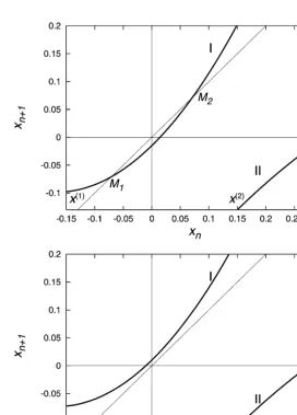
2.2.1. Intermittency as a result of a tangent bifurcation

It is well known that one possible route for the loss of stability of regular motion and the onset of chaos in dynamical systems is the fusion of a stable steady state with an unstable one, with the subsequent disappearance of both of these states. In certain conditions after this bifurcation, which is often said to be tangential, the motion of the system exhibits the property ofintermittency(see, for example, [50}52]). This property implies that in the system phase space the representative point is

Fig. 1. Sketch of a model map close to the transition through intermittency: (a) before the transition; and (b) after the transition.

bifurcation point the duration of the laminar phases decreases and that of the turbulent ones increases until, "nally, the laminar phases disappear altogether. The dependence of the mean

duration of the laminar phases on the excess of the bifurcation parameter beyond its critical value can be evaluated by using a model map (see, for example, [53}55,35,36,52]). If the system is acted

upon by weak noise then the mean duration of the laminar phases is also dependent on the noise intensity. We will concentrate on the results of [35,52], in which the theory of the passage through a boundary was used.

Let us consider a system described by a one-dimensional map that can be presented as shown in Fig. 1 close to the bifurcation point. At the bifurcation point a stable"xed point of the map,M₁,

5The sense ofx(1)andx(2)is clear from Fig. 1.

6The authors of [53] set an unjusti"ed second boundary condition w(x(1))"_{0 and added a constant source in}

Eq. (2.52).

the map touches the bisectrix. For su$ciently smalle, Dx(1)DandDx(2)D5the part of the map labeled

I can be approximated as

x_n`1"e#x

n#axqn, (2.49)

where q is an even number. It is evident that laminar phases are associated with motion of the representative point along part I of the map, whereas turbulent phases are associated with transitions of the representative point to the part labeled II and back again. It has been shown [54,55] by using a renormalization T-group technique that the mean durationqof laminar phases is proportional toe~(1~1@q). The same result is obtained in [53,35,52] by replacing the di!erence

equation (2.49) by the corresponding di!erential equation. In [53}55,35,52] the in#uence of

external noise is also considered. It is found that, for e"0,q&g~2(q~1)@(q`1).

The presence of external noise can be described by an additional term in Eq. (2.49), namely

x_n`1"e#x

n#axqn#gm

n, (2.50)

wherem_nis white noise with zero mean. We assume thatSm_nm_mT"d

nm, wherednmis the Kronecker

delta. For su$ciently smalle,ganda(x(1),(2))qEq. (2.50) can be replaced by the following di!erential

equation [53,35]:

x5"e#axq#gm(t) , (2.51)

where Sm(t)T"0, Sm(t)m(t@)T"d(t!t@). The Fokker_}Planck equation for the probability density

w(x,t) associated with Eq. (2.51) for x4x(2)is

Rw

Rt"!

R

Rx((e#axq)w)# g2

2 R2w

Rx2 . (2.52)

To calculate the mean duration of laminar phases it is su$cient to"nd a steady-state solution of

Eq. (2.52) satisfying the normalization condition and the zero boundary condition at the point

x"x(2).6 Because all points attaining the boundaryx(2) leave the interval in question, we put

w(x(2))"0 . (2.53)

For x(1)4x4x(2) the steady-state solution of Eq. (2.52) with the boundary condition (2.53) is

w(x)"2G0

g2 exp

C

2

g2

A

axq`1

q#1

BDP

x(2) x

exp

C

g2

A

ayq`1

q#1

BD

whereG₀ is the value of the probability#ux

G"(e#axq)w!g2

2 dw

within the intervalx(1)4x4x(2). Forx(x(1)the probability_#ux is equal to zero, and therefore

w(x)"2G0

g2 exp

C

2

g2

A

axq`1

q#1

BDP

x(2) x(1)

exp

C

g2

A

ayq`1

q#1

BD

The value of the probability#uxG₀is determined from the normalization condition by integrating

(2.54) and(2.55) with respect toxfrom!Rtox(2). It follows from the general theory of_#uctuational

transitions set forth above that the mean duration of laminar phases qis equal toG~1₀ . Thus,

q"2

g2

AP

x(2) x(1)

exp

C

g2

A

axq`1

q#1

BDP

x(2) x

exp

C

g2

A

ayq`1

q#1

BD

#

P

(1)

~=

exp

C

g2

A

axq`1

q#1

BD

P

x(2) x(1)exp

C

!2

g2

A

ayq`1

q#1

BD

B

In the simplest case wheng,0, i.e., in the absence of external noise, it immediately follows from

Eq. (2.52) that

w(x)"

G

G₀

e#axq for x(1)

4x4x(2) ,

0 for x(x(1) .

(2.57)

It can be seen from (2.57) that in the speci"c case whenq"2 the probability distribution takes the

form of a Lorentzian with its maximum atx"0; the width of this line is equal toJe/a. The value

ofG₀in (2.57) can be calculated explicitly for su$ciently smallewhen we can putx(1)+!Rand x(2)+R. In this case we_"nd

q+ 2p

qsin(p/q)(aeq~1)~1@q . (2.58) For q"2 we haveq&e~1@2. In another speci_"c case whene"0, gO0 we obtain from (2.56):

q"2(q~1)@(q`1)

A

#1

a

B

2@(q`1)

Bg~2(q~1)@(q`1), (2.59)

whereB is determined by the formula

B"

P

u1

exp(uq`1)

P

u

exp(!vq`1) dvdu#

P

~=

exp(uq`1) du

P

exp(!vq`1) dv ,

u_1,2"

A

(q#1)g2

B

1@(q`1)

x(1),(2).

For su$ciently small external noise, wheng2;aDx(1),(2)Dz`1we can putu₁+!Randu₂+R. In

this caseBis independent ofgand we have from (2.59)q&g~2(q~1)@(q`1). In particular, forq"2,

q&g~2@3.

2.2.2. On}owintermittency

Recently another type of intermittency was discovered. It is known ason}owintermittency. This

intermittent behavior was"rst considered by Pikovsky [57] and then by Fujisaka and Yamada

[58]. An important point is that this type of intermittency can occur not only in coupled dynamical systems but in stochastic systems as well [59]. In [59] the statistical properties of on}o!

intermittency were studied through analysis of the map

x_n`1"a(1#y

n)xn#f(x

n) , (2.60)

where y_n is either a deterministic chaotic process or a random process, a is the bifurcation parameter, and f(x_n) is a nonlinear function free from a linear term. For this map it was shown that for a'0 the mean duration of laminar phases is proportional to a~1. The in_#uence of

weak additive noise on the characteristics of on}o! intermittency was considered by Chenis and

Lustfeld [60].

We consider on}o! intermittency by reference to a speci"c example system described by the

following model equations:

x5"!(b#ar2)x#x

A

1(t)#m2(t)

r

B

A

m₂(t)

r

B

where r"Jx2#y2, and m

1(t) and m2(t) are white noises of intensities i1 and i2, respectively.

Eqs. (2.61) can be rewritten in polar coordinatesr and u"arctan(y/x) as

r5"!(b#ar2)r#rm

1(t)#m

2(t), u5"0 . (2.62)

We see that m₁(t) and m₂(t) represent multiplicative and additive noise respectively. The "rst of

Eqs. (2.62) is of the same form as (2.7). Hence, the Fokker}Planck equation associated with this

equation can be written as

Rw

Rt"!

R

Rr((ba!ar2)rw(r,u,t))#

1 2

R2

Rr2((r2i1#i2)w(r,u,t)) , (2.63)

wherea"i

1/2b!1 is the bifurcation parameter. To calculate the mean duration of the laminar

phases, we assume that our system is in a laminar phase ifr4e, whereeis a given small quantity.

The mean duration q

e of the laminar phases is determined by the mean duration of a random

walk-like motion of a representative point on the phase plane xy inside a circle of radius e. As shown above, this duration can be calculated by using the steady-state solution of Eq. (2.63) with the boundary condition

w(r,u)D_r/e"0 . (2.64)

This solution is

w(r,u)"2G

i₁

A

k 2(a#1)

B

(ak`i1a)@2(a`1)i1~1

exp

A

i₁

B

]

P

r

A

# k

2(a#1)

B

~(ak`i1a)@2(a`1)i1

exp

A

i₁

B

e, k"i

expression (2.65) over the circle of radiuse:

G~1"4p

i₁

P

e

0

r

A

2(a#1)

B

(ak`i1a)@2(a`1)i1~1

exp

A

i₁

B

]

P

r

A

# k

2(a#1)

B

~(ak`i1a)@2(a`1)i1

exp

A

i₁

B

r"e is determined by total probability _#ux across this boundary, i.e., ¹"(2peG)~1. Taking

account of the fact that the representative point touching the boundary can return again with probability (1!p), we obtain for the mean duration q of the laminar phases the following

expression [38,39]:

q"¹p+=

j/1

j(1!p)j~1 .

Summing the series we have

q"¹/p . (2.67)

Let us consider the speci"c case whenae2/i₁;1. We can then ignore the terms exp(!ar2/i₁) and

exp(ao2/i₁). As a result we obtain

¹" 2

i₁e

P

e

0

r

A

2(a#1)

B

(ak`i1a)@2(a`1)i1~1

P

r

A

# k

2(a#1)

B

~(ak`i1a)@2(a`1)i1

dodr . (2.68)

To calculate the inner integral approximately, we multiply and divide the integrand byo, substitute

y foro2 and takee/2 in place of o. This manipulation gives

¹" 2(a

#1)

i₁(a#2)!ak

G

2i₁(a#1)

i₁a#ak

A

# k

2(a#1)e2

B

]

C

A

2(a#1)e2#k

B

(i1a`ak)@2(a`1)i1

D

H

In particular, fork"0 (additive noise is absent) we obtain from (2.69) the following simple formula:

¹"1/ba . (2.70)

So, fork"0, we have the same dependence ofqonaas for the map (2.60); whereas, forkO0, the

dependence is more complicated. Forkb;e2i

1we have¹"2(a#1)/(i

1a#ak), i.e., nonlinearity

plays an important role in this dependence, given that the intermittent behavior begins to show itself fora(a

#3"0. In another limiting case, whenkb<e2i

1,¹"e2/2i

2, i.e., for very smalleor

i₁ the mean duration of laminar phases is independent of a. For a"0,ak;b we obtain from

(2.70) the following dependence of¹on the intensity of additive noise, conveniently characterized

by the parameteri"k/2e2:

¹"1

b

A

1#i

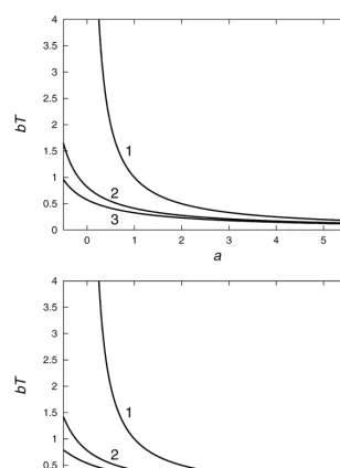
Fig. 2. Dependence ofb¹_{onain the case where}ae2_/i

1;_{1 for}i

2"_{0 (curves labelled 1),}i

2"_{0.1 (curves labelled 2),} i"0.2 (the curves labelled 3), for: (a)b"0; and (b)b"1.

i.e., the decline of the mean duration of laminar phases with increasing intensity of additive noise is logarithmic in character. The dependences ofb¹onafor di_!erent values ofi

2constructed by the

formula (2.69) are shown in Fig. 2 for two cases: (a) when the nonlinearity characterized by the parameterb"ae2/b can be neglected, and (b) when it is taken into account. We see that the

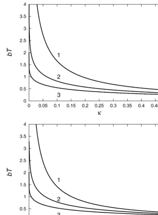
nonlinearity exerts only a small in#uence on these dependences. The dependences ofb¹oni₂for

Fig. 3. Dependence ofb¹oni

2in the case whereae2/i1;1 fora"!0.5 (curves labelled 1),a"0 (curves labelled 2),

a"0.5 (curves labelled 3), for: (a)b"0; and (b)b"1.

3. Noise-induced transport of Brownian particles(stochastic ratchets)

In recent years#uctuation-induced transport phenomena for Brownian particles have attracted

considerable interest, usually in the context of biological and chemical problems (see, for example, [61}66,20,22,24]). A physical experiment demonstrating the possibility of such transport in

a ratchet-like potential "eld created by laser beam is described in [67]. In [68] it was

a periodic asymmetric potential (more recently, this phenomenon become known as a yashing

ratchet). Similar experiments are also presented in [69].

Systems in which noise-induced transport occurs are often called stochastic ratchet-like devices by analogy with mechanical device_`ratchet and pawl_adescribed and considered by Feynman [70]. Feynman showed that in the case of thermodynamic equilibrium the ratchet on average is at rest

}it advances and retreats by an equal number of teeth on the wheel}as it must be because of the

Second Law of Thermodynamics. It is interesting that similar considerations were discussed by Smoluchowski [71] well before Feynman. The_`ratchet and pawl_adevice constitutes a mechanical recti"er. It is similar in essence to an electrical recti"er. However, as is often the case, the problems

associated with electrical recti"cation of#uctuations were discussed independently of the ratchet

problems [72}77]. In [73,74] it was found that in the simplest electrical recti"er, consisting of

capacitor and diode, the capacitor can be charged without an external source, at the expense of only thermal #uctuations. This paradoxical result cast some doubt on the applicability of the

Second Law of Thermodynamics to the phenomenon considered [76]. As far back as 1950, however, considering the diode as a nonlinear resistor, Brillouin [72] showed that, for the Second Law to apply, a shift of the characteristic of the nonlinear resistor must be taken into account. Stratonovich [77,78] established, on a certain model of diode, that such a shift does indeed occur due to #uctuations of the current through the diode considered as a nonlinear resistor, and he

calculated it. With this shift, the mean value of the voltage drop across the capacitor is found to vanish for the case of thermodynamical equilibrium.

Most commonly, consideration of noise-induced transport is restricted to the so-called overdam-ped case, when the mass of the Brownian particle can be neglected and its motion is described by a "rst order di!erential equation of the form

x5#f(x)"u(t)#f(x,t)#m(t) , (3.1)

wheref(x) is a periodic function ofxpossessing an asymmetry,u(t) is a regular periodic force,f(x,t) is a random process with zero mean value, andm(t) is white noise of intensityKimitating thermal

#uctuations. The processf(x,t) can be either given or described by additional equations.

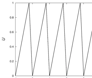
More often than not researchers of noise-induced transport set the function f(x) to a form corresponding to a saw-tooth potential;_(x)":x

0f(x) dx shown in Fig. 4. In this case

f(x)"

G

a₁ for n¸(x(n¸#x

1 ,

!a

2 for n¸!x

2(x(n¸ ,

(3.2)

wheren"0,$1,$2,₂,¸"x

1#x

2is the period of the functionf(x). It is easily shown that, in

the absence of the disturbancesf(x,t) andm(t), the pointsx"n¸andx"n¸#x

1"(n#1)¸!x

2

correspond to stable and unstable equilibrium states, respectively. If there are #uctuations then

transitions from one stable state to another can occur. Directional motion of the particle will occur if the probabilities of transitions in opposite directions are di!erent. So, we see that the problem of

noise-induced transport is closely allied to the#uctuational transitions considered above.

It is usual to distinguish two types of ratchet devices [64,79,65,20,80]: (a) wheref(x,t) is a force independent ofx; and (b) wheref(x,t) depends onx. In its turn, the latter can be also divided into two subclasses: (i) those where f(x,t)"f(x)s(t), which is to say that the height of the potential

Fig. 4. An example of a saw-tooth potential;(x).

In the last few years much attention has been concentrated on the possibility of exploiting such phenomena to separate particles of di!erent mass or size. In this connection studies of di!erent

models giving #ux reversals as the system parameters change are very important [81}83,85,86].

Flux reversals induced by noise colour alone, predicted in [82], were subsequently observed in analogue electronic experiments [84].

We consider below the one-dimensional motion of a Brownian particle in a viscous medium described by the following equation:

kxK#x5#f(x)"u(t)#f(x,t)#m(t) , (3.3)

wherek"m/b,mis the particle mass,bis the viscous friction factor,f(x) is described by expression

(3.2), and u(t), f(x,t) and m(t) are the same that in Eq. (3.1). For k"0 this equation reduces to

Eq. (3.1).

3.1. Noise-induced transport of light Brownian particles in aviscous medium

with a saw-tooth potential

Here we consider the case when viscous friction in the medium is su$ciently large and mass of

the particle is su$ciently small, that the motion of the particle can be described approximately by

withm(t). The Fokker}Planck equation associated with Eq. (3.1) at the speci"ed conditions is

Rw

Rt"!

R

Rx

AA

K₁

2 f(x)f@(x)

B

B

R2

Rx2(K(x)w(x,t)) , (3.4)

where K(x)"K#f2(x)K

1. Because f(x) is a periodic function of x, w(x,t) is also a periodic

function ofx. Thus Eq. (3.4) only needs to be solved within the interval from!x

2 tox1.

Let us show that the statistical average of the particle velocityx5 is determined by the relationship

Sx5 T"

P

~x2

G(x,t) dx, (3.5)

where

G(x,t)"!1

2

R(K(x)w(x,t))

Rx #F(x,t)w(x,t) (3.6)

can be treated as the instantaneous probability#ux,F(x,t)"u(t)!f(x)#(K₁/2)f(x)f@(x).

Aver-aging Eq. (3.1) over statistical ensemble and taking into account that the random processm(t) has zero mean value andSf(x,t)T"(K

1/2)f(x)f@(x), we obtain

Sx5 T"SF(x,t)T"

P

~x2

F(x,t)w(x,t) dx.

According to (3.6), this expression can be rewritten as

Sx5 T"

P

1

~x2

F(x,t)w(x,t) dx"

P

1

~x2

A

G(x,t)#1

2

R(K(x)w(x,t)) Rx

B

Because of the spatial periodicity of the functions w(x,t) and K(x) we obtain the formula (3.5). Averaging (3.5) over time we have

Sx5 T"

P

~x2

G(x,t) dx, (3.7)

where

G(x,t)"lim

T?=

1

¹

P

T 0

G(x,t) dt.

So, the mean particle velocity, i.e., its net di!usive drift, is proportional to the probability #ux

averaged over both space and over time.

3.1.1. The case of an additional regular force We now consider the case whenK

1"0 andu(t)O0. If the functionu(t) is su_$ciently slow, we

can use the successive approximation technique for solving Eq. (3.4) by putting

w(x,t)"w

0(x,u)#w

1(x,u)u5#w

As a zeroth-order approximation, we take a quasistationary solution of Eq. (3.4) for which

Rw/_Rt"0. In this approximation we obtain the following equation forw

0(x,u): K

2

Rw₀(x,u)

Rx !(u!f(x))w0(x,u)"!G0(u) , (3.9)

whereG₀(u) is the probability#ux in the zero approximation. Solving Eq. (3.9) with account taken

of (3.2) we"nd

w₀(x,u)"

G

A

q

1

B

exp

A

K

B

G₀(u)

q 1

for 04x4x

1,

A

q₂

B

A

2q₂x

K

B

G₀(u)

q₂ for !x24x40 ,

(3.10)

where

q_1,2"uGa

1,2, (3.11)

andC₀(u) is an arbitrary function ofu. From the periodicity condition of the functionw₀(x,u) we

"nd the relation betweenG₀(u) andC(u): C₀(u)"Q(u)G₀(u), where Q(u)" 1

q₁q₂

q₂exp(2;

0u/Ka1)!q

1exp(!2;

0u/Ka2)!(q

2!q

1) exp(2;0/K)

exp(2;

0u/Ka1)!exp(!2;

0u/Ka2)

, (3.12)

and ; 0"a

1x1"a

2x2 is the height of the potential barrier. The probability #ux G₀(u) can be

found from the normalization condition for the probability densityw₀(x,u). In so doing we obtain

G~1

0 (u)";

0

A

1

a₁q₁#

1

a₂q₂

B

K(a₁#a

2)2

2q21q22 exp

A

2; 0

K

B

](exp(2;0u/Ka1)!exp(2;

0/K))(exp(!2;

0u/Ka2)!exp(2;

0/K))

exp(2;

0u/Ka1)!exp(!2;

0u/Ka2)

. (3.13)

In the most interesting case when uis su$ciently small, namely when

maxu; a1a2

a₂!a

1

min

A

0

B

, (3.14)

we "nd

G₀(u)"G

00u#G

01u2#2, (3.15)

where

G₀₀"

; 0a1a2

K2(a₁#a

2)sinh2(;0/K)

,

G₀₁"G

00

a₂!a

1

a₁a₂

A

;20

K2sinh2(;

0/K)

#

; 0 Ktanh(;

0/K)

!2

B

For simplicity, we further restrict ourselves to the case when condition (3.14) is valid. In this case, we have from (3.12), (3.11), (3.15) and (3.8)

C₀(u)"C

00#C

7Here we have taken into account that, as follows from the normalization condition for the functionw(x,t), the integrals ofw

1(x,u),w21(x,u) andw22(x,u) with respect toxbetween the limitsx"!_x

2andx"_x

1must be equal to

zero.

where

C₀₀" 2a1a2

K(a₁#a

2)(1!e~2U₀@K), C01 "a2

!a

1

a₁a₂ C00

A

;20

K2sinh2(;

0/K)

!1

B

w(x,t)"w

0(x,u)#(w

10(x)#w

11(x)u)u5 #(w

20(x)#w

21(x)u)uK #w₂₂(x)u5 2#2. (3.18)

It follows from (3.8) and (3.18) that the functions w

10(x), w11(x), w20(x), w21(x), and w22(x) are

described by the equations

K

2

dw₁₀(x)

dx #f(x)w10(x)"!G10(x), G10(x)"!

P

Rw₀(x,u)

Ru

K

K

2

dw₁₁(x)

dx #f(x)w11(x)"!G11(x), G11(x)"!

P

R2w₀

Ru2

K

K

2

dw₂₀(x)

dx #f(x)w20(x)"!G20(x), G20(x)"!

P

w₁₀(x) dx#G

20, (3.21)

K

2 dw

21(x)

dx #f(x)w21(x)"!G21(x), G21(x)"!

P

w₁₁(x) dx!w

20(x)#G

21, (3.22)

K

2

dw₂₂(x)

dx #f(x)w22(x)"!G22(x), G22(x)"!

P

w₁₀(x) dx#G

22. (3.23)

So, for smallu we"nd

Sx5 T+G

0¸#B2u2

2

P

x1 ~x2

(G₂₂(x)!G

21(x)) dx"

A

0#G

2

B2u2

2

B

22!G

21.7Thus, the correction to the quasistationary solution is proportional to the

frequency squared and to the value ofG₂. Subtracting (3.22) from (3.23) we obtain the equation for =_(x),w

22(x)!w

21(x): K

2

d=_(x)

dx #f(x)=(x)"!(w20(x)#G2) . (3.25)

A solution of this equation is

=_(x)"

G

A

a₁!

2

K

P

x 0

w₂₀(x@) exp

A

K

B

B

A

2a₁x

K

B

G₂

a₁ for 04x4x1,

A

a₂!

2

K

P

x 0

w₂₀(x@) exp

A

K

B

B

A

2a₂x

K

B

G₂

a₂ for !x24x40 .

From the periodicity condition we "nd G₂:

G

2"! 2a1a2

K(a₁#a

2)(e2U0@K!1)

P

x1 ~x2

w

20(x) exp

A

2f(x)x

K

B

So, to calculateG₂ we must "nd w₂₀(x) which in turn is determined by Eq. (3.21). To solve this

equation we must previously have solved Eq. (3.19). Although this procedure is simple in principle, it leads to rather cumbersome expressions. Therefore we restrict ourselves to the analysis of the zeroth-order approximation. If condition (3.14) is ful"lled and u(t),B₀"const (in addition to f(x) a constant force acts upon the particle), then

Sx5 T+

;20

K2sinh2(;

0/K)

B₀, (3.28)

i.e., the particle moves in the direction of this constant force no matter what the relation between

a₁ and a₂. We see from (3.28) that in the absence of #uctuations, when KP0,Sx5 TP0, i.e.,

transport of the particle is impossible despite the presence of the constant force. This is because the force is small and cannot by itself push the particle over the potential barrier. In another speci"c

case, when u(t)"Bcosut, whereB is su_$ciently small, we obtain

Sx5 T+

;20_(a 2!a

1)B2

2K2a₁a₂sinh2(; 0/K)

A

;20

K2sinh2(;

0/K)

#

; 0 Ktanh(;

0/K)

!2

B

i.e., the particle moves in the direction of the slower rate of potential change. It is easy to verify that, in the absence of#uctuations, transport of the particle cannot occur, just as in the case of a small

constant force.

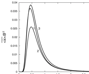
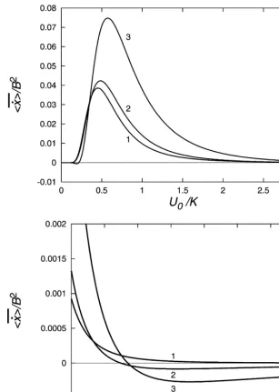
Examples of the dependences ofSx5 T/B2onK/;

0described by formulas (3.7), (3.13) are shown in

Fig. 5 for a number of values ofB. We see that these dependences are of radically di!erent kinds for

B(min(a

1,a2) and B'min(a

1,a2). In the "rst case these dependences have a maximum at

a certain value ofK/;

0that is the smaller the greater isB. ForK/;0P0, i.e., in the absence of the

thermal #uctuations, Sx5 T/B2P0. In the second case Sx5 T/B2 tends to a certain "nite value as

K/;

0P0, which can be calculated from the theory of vibrational transport [87,86]. ForB(0.5

the dependences found are almost coincident with those described by the approximate formula (3.29). In this case the averaged particle velocity is maximal forK/;

0+0.43. In the case thatB(min (a

1,a2),

the ratioK/;

0 is either very small or very large, noise-induced transport is not feasible.

The results obtained can be explained in the following manner. Noise-induced transport can occur if#uctuational transitions through each potential barrier are more frequent in one direction

than in another. Because the probability of the transition through a certain potential barrier depends only on its height and the intensity of#uctuations, transport is impossible in the absence of

the additional forceu(t). In the case of a constant force the result is self-evident because the heights of the potential barriers for the particle moving rightwards and leftwards are di!erent. The case of

an alternating force is more complicated. During one half-period the right potential barrier is lowered to;

0!Bx

1, whereas the left one rises to;0#Bx

2. During the next half-period the

right potential barrier rises to ;

0#Bx

1, whereas the left one is lowered to ;0!Bx

2. Because

Fig. 5. Dependence ofSx5 T/B2onK/;

0as described by Eqs. (3.7) and (3.13) fora1"1.25,a

2"5,x

1"0.8,x

2"0.2, and:

B"0.1 (curve 1);B"1 (curve 2);B"2 (curve 3); andB"5 (curve 4).

We note that a similar problem forB₀"0 was solved numerically in [81] by use of the so-called

matrix continued fraction technique. It was shown that, for low frequencies, the numerical results coincide with quasistationary approximation (in [81] it is called the adiabatic approximation). But for high frequencies the results obtained were radically di!erent in character; for example,

a reversal of the probability#ux over certain ranges of K/;₀ and Bwas detected.

3.1.2. The case of random modulation of the potential barrier height

For simplicity assume that in Eq. (3.1) the regular forceu(t) is absent. In this case a stationary solution of the Fokker}Planck equation (3.4) satisfying the continuity condition forx"0 is

w(x)"

G

a₁

A

A

2a₁x

K(1)

BB

A

2a₁x

K(1)

B

G a

2

A

1!exp

A

K(2)

BB

A

2a₂x

K(2)

B

(3.30)

where

K(1,2)"K#K

From the periodicity condition for the functionw(x) we"nd the relation betweenGand C:

G

C

A

A

; 0

K(2)

BB

A

A

2; 0

K(1)

BBD

"Ca

1a2

C

A

; 0

K(1)

B

A

2; 0

K(2)

BD

Taking account of (3.30) and (3.31), and from the normalization condition, we "ndG:

G" 2a21a22

a₁#a

2

C

exp

A

; 0

K(1)

B

A

2; 0

K(2)

BDG

C

A

2; 0

K(1)

BD

]

C

A

; 0

K(2)

BD

C

A

2; 0

K(1)

B

A

2; 0

K(2)

BDH

~1

. (3.32)

It follows from (3.32) thatSx5 T"G¸O0 only ifa

1Oa

2andK1O0. The dependences ofSx5 Ton

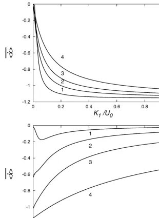
K₁for di!erent values ofK/;₀, and onK/;₀ for a number of"xed values of K₁, are shown in

Fig. 6. It is interesting that the particle moves on average in the direction of the greater rate of the potential change. We draw attention to the fact that, for random modulation of the potential barrier, the directional di!usion of particles is possible even in the absence of thermal#uctuations

(K"0).

3.1.3. The case of an additional random force of large correlation time

Fluctuational transport of a Brownian particle in a viscous medium induced by thermal noise and a correlated random force that is a Markov process was studied in [79]. However, concrete results were obtained only for dichotomous and _`kangaroo_a-like processes. We suggest here a way of tackling this problem for the case where the correlated random force is the so-called Ornstein}Uhlenbeck process [88]. We can then write the following equations of

motion:

x5#f(x)"y#m(t) , (3.33)

y5"!cy#m

1(t) , (3.34)

wheref(x) is determined by expression (3.2), andm(t) andm₁(t) are uncorrelated white noises with zero mean values and intensities equal toKandK₁respectively. The stationary probability density of the variableyis independent ofxand can be easily calculated from the Fokker}Planck equation

associated with Eq. (3.34). It is equal to

p(y)"

S

pK₁exp

A

cy2

K₁

B

Let us calculate now the conditional probability density of the variablexfor a"xed value ofy. In

the quasistationary approximation, which is valid for su$ciently large correlation time of the

processy(t), this probability densityw(xDy) satis"es the following Fokker}Planck equation:

G(y)"!(f(x)!y)w(xDy)!K

2

Rw(xDy)