On Solving Systems of Autonomous Ordinary Differential Equations by Reduction to a Variable of an Algebra

(1)

Volume 2012, Article ID 753916,21pages doi:10.1155/2012/753916

Research Article

On Solving Systems of Autonomous

Ordinary Differential Equations by Reduction to

a Variable of an Algebra

Alvaro Alvarez-Parrilla,

1, 2

_{Mart´ın Eduardo Fr´ıas-Armenta,}

3

Elifalet L ´opez-Gonz ´alez,

4

_{and Carlos Yee-Romero}

1

1_{Facultad de Ciencias, Universidad Aut´onoma de Baja California, Km. 103 Carretera Tijuana-Ensenada,}

22860 Ensenada, BC, Mexico

2_{Grupo Alximia SA de CV, Departamento de Investigaci´on, Ryerson 1268, Zona Centro,}

22800 Ensenada, BC, Mexico

3_{Departamento de Matem´aticas, Universidad de Sonora, 83000 Hermosillo, SON, Mexico}

4_{División Multidisciplinaria de la UACJ en Cuauhtémoc, Universidad Autónoma de Ciudad Juárez,}

32310 Ciudad Ju´arez, CHIH, Mexico

Correspondence should be addressed to Alvaro Alvarez-Parrilla,[email protected] Received 26 March 2012; Accepted 16 May 2012

Academic Editor: Mihai Putinar

Copyrightq2012 Alvaro Alvarez-Parrilla et al. This is an open access article distributed under the Creative Commons Attribution License, which permits unrestricted use, distribution, and reproduction in any medium, provided the original work is properly cited.

A new technique for solving a certain class of systems of autonomous ordinary differential equations overKn_{is introduced}_K_{being the real or complex field}_{. The technique is based on two} observations:1, ifKn_{has the structure of certain normed, associative, commutative, and with a} unit, algebrasAoverK, then there is a scheme for reducing the system of differential equations to an autonomous ordinary differential equation on one variable of the algebra;2a technique, previously introduced for solving differential equations overC, is shown to work on the class mentioned in the previous paragraph. In particular it is shown that the algebras in question include algebras linearly equivalent to the tensor product of matrix algebras with certain normal forms.

1. Introduction

Throughout this work,Kwill stand for a field, usually the realRor the complex fieldC. Consider the autonomous ordinary diﬀerential equation

dx

dt fx, x∈Ω⊂K

n_{, t}_∈_R_, _1.1

(2)

In general the solution is not easy to obtain since this is usually a system of coupled differential equations. There is a vast literature regarding the solution of ordinary differential equations by different means and in particular by techniques utilizing generalized

analytic functions, see for instance1–14. These include applications to the three-dimensional Stokes problem, solutions of planar elliptic vector fields with degeneracies, the Dirichlet problem, multidimensional stationary Schr ¨odinger equation, among others3,5,6,12,13. In particular, the technique that we present is of interest for people working on vector fields with singularities. For instance, in order to gain insight into the behaviour of analytic vector fields, correct visualization of vector fields in the vicinity of their singular set is required, in the case of visualization of two-dimensional complex analytic vector fields with essential singularities the usual methods only provide partial resultssee15–17, whilst the technique which we promote provides accurate and correct solutions18,19. These questions arise naturally in discrete and continuous dynamical systemssee20–22.

As a first step in obtaining a solution to1.1, we notice that, ifKn _{can be given the} structure of a certain algebraA, it is possible to reduce this system to a single autonomous diﬀerential equation

dζ

dt gζ, ζ∈Ω

_⊂_A_{, t}_∈_R_, _1.2

withgbeing a functionA-diﬀerentiable with respect to the variableζin the algebraA. Having done so, we proceed to show that it is possible to solve1.2by extending a geometric technique introduced in18,19in the context of complex analytic vector fields related to Newton vector fields which are first studied by 23. This technique is based upon the construction of two functions, which, are respectively, constant and linear on the trajectories which are the solutions of1.2.

The paper is organized as follows. In Section2the algebras in question are introduced, in particular we introduce the notion of normed, associative, commutative, and with a unit, finite dimensional algebraAoverK, showing in Section2.1that these have a first fundamental

representation into the algebra ofn×nmatrices overK,Mn,K. Furthermore in Section2.2

normal algebras are defined and their corresponding tensor products are constructed. This is

standard material which can be found in24–26but is presented here for completeness. In Section3we give the definition ofA-differentiability, and proceed to show that if the family of matrices {Jfx : x ∈ Ω} is linearly equivalent to a subset of an algebra B inMn,K, that is, the image of the first fundamental representation of an algebraAwith respect to the canonical basis ofKn_{, that is,}_B_R_A_{, then in fact}_f_is_A_-di_ff_{erentiable on}_Ω_. The problem of determining if a mapf :Ω⊂Kn _→ _Kn_is_A_-di_ff_{erentiable for some algebra}

Ais treated indirectly in27, where the conditions that are given ensure the existence of an algebraAsuch that the set of relations are the generalized Cauchy-Riemann equations for

A,27,28show that these equations give a criterion forA-diﬀerentiability. Furthermore

(3)

In Section5we start by showing that in this context the diﬀerential equation1.1takes the form

dζ

dt gζ, ζ∈Ω

_{\ S ⊂}_A_{, t}_∈_R_, _1.3

withgbeing a functionA-diﬀerentiable with respect to the variableζin the algebraA, andS being a certain singular set, where the solutions are not defined.

We then proceed to show that the geometric technique, introduced in 18, 19, of finding two functionsh1andh2which are constant and linear on the trajectoriesζtwhich

are solutions of the diﬀerential equation, can be extended to the case of 1.3. We end the section and the paper with an example.

2. Algebras

We introduceK-algebrassee, e.g.,24.

Definition 2.1. A K-algebra or algebra over K is a finite dimensionalK-linear spaceA on which is defined a bilinear mapA×A → Athat is associative and commutative, and there is a unit elementeeAinAthat satisfiesexxexfor allx∈A.

An element a ∈ A is called regular if there exist a unique element inAdenoted by a−1∈Acalled inverse ofasuch thata−1aaa−1e. An elementa∈Awhich is not regular is called singular. Ifa, b∈Aandbis regular, the quotienta/bwill meanab−1.

2.1. Algebras and Their Fundamental Representations

We define the first fundamental representation.

IfB{β1, . . . , βn}is an ordered basis of an algebraA, the product between the elements ofBis given by

βiβj n

k1

cijkβk, 2.1

where cijk ∈ K for i, j, k ∈ {1,2, . . . , n} are called the structure constants of A. The first

fundamental representation ofAassociated toBis the isomorphismR:A → Mn,Kdefined by

Rx1β1 x2β2 · · · xnβn

x1R1 x2R2 · · · xnRn, 2.2

whereRiis the matrix whose entryj, kiscijkfori1,2, . . . , n. The commutativity and the associativity ofAare equivalent to the identities

1cijk cjik, for alli, j, k∈ {1,2. . . , n}and

2_lcijlclkslcjklcils, for alli, j, k, s∈ {1,2. . . , n},

(4)

UsingR we assign toAthe norm induced from the operator norm inMn,K see

24. In this way each algebra is a normed algebra, that is, there exists a norm · :A → R satisfyingxy ≤ xyfor allx, y∈Aande1.

Example 2.2. Let A be the linear space R3 _{with the product between the elements of the}

standard basisB{e1, e2, e3}given in the following equation:

e1 e2 e3

e1 e1 e2 e3

e2 e2 −2e1 2e2 e3 −e1 e2 e3

e3 e3 −e1 e2 e3 −e1 2e3

, 2.3

that extends to the product inR3given by

x, y, zu, v, w e1x, e2y, e3z

e1u, e2v, e3w

xue1e1 xve1e2 xwe1e3 yue1e2 yve2e2

ywe2e3 zue1e3 zve2e3 xwe3e3

xu−2yv−yw−zv−zwe1

xv−yu−zyv−yw zve2

zw zu yv yw zv zwe3.

2.4

The product between the elements ofBdefine the structure constantscijk fori, j, k ∈

{1,2,3}. So,R3_{with the product given is an algebra}_A_.

2.2. Normal Algebras and Their Tensor Products

LetB1, B2, . . . , Blbe matricesBi∈Mki,K, eachBiof one the following four types:

r,

⎛ ⎜ ⎜ ⎜ ⎜ ⎜ ⎜ ⎝

s 0 0 · · · 0

1 s 0 0

0 1 s 0

..

. . .. 0 0 0 · · · s

⎞ ⎟ ⎟ ⎟ ⎟ ⎟ ⎟ ⎠ ,

a −b b a , ⎛ ⎜ ⎜ ⎜ ⎜ ⎜ ⎜ ⎝

C 0 0 · · · 0

I2 C 0 0

0 I2 C 0

..

. . ..

0 0 0 · · · C

⎞ ⎟ ⎟ ⎟ ⎟ ⎟ ⎟ ⎠

, 2.5

where

C

u −v v u

, I2

1 0 0 1

(5)

r, s, a, b, u, v∈Kandk1 · · · kln. In this case we will say that the matrixBgiven by

B

⎛ ⎜ ⎜ ⎜ ⎝

B1 0 · · · 0

0 B2 0

..

. . .. 0 0 · · · Bl

⎞ ⎟ ⎟ ⎟

⎠, 2.7

is in its normal form. We will associate toBan algebra of matrices of dimensionnoverKwhich containsBand use the following nomenclature: The first block will be called real simple block, the second real Jordan block, the third simple complex block, and the fourth complex Jordan block.

For i 1,2, . . . , l, let σi : Mki,K → Mn,K be the linear sections defined by substituting the matrixM ∈ Mki,Kin the block Bi of the matrix Band taking the other entries as zero. The real Jordan block may be written in the following wayBi aiDi Ni, whereDi is the identity andNi is a nilpotent matrix of orderki. The simple complex block may be written in the formBi aiDi biJi, whereDiis a diagonal matrix andJi is a matrix withJ2

i −Di. The complex Jordan blocks may be written in the formBi aiDi biJi Ni, whereDiis the identity andJiis a matrix withJ_i2 −DiandNiis a nilpotent matrix of order

ki/2.

We define the matrices{βi,j : 1≤i≤l, 1≤j ≤ki}whose entries are in the blockBias follows.

iIfBiis a real simple block,βi,1:σi1, in this caseki1.

iiIfBiis a real Jordan block,βi,1:σiDiandβi,j :σiN_ij−1forj2, . . . , ki.

iiiIfBiis a simple complex block,βi,1:σiDiandβi,2:σiJi.

ivIfBi is a complex Jordan block,βi,1 :σiDi,βi,2 :σiJi,βi,2j−1 :σiN2_ij−1, and

βi,2j:βi,2σiN_i2j−1forj2, . . . , ki/2.

Observe that the product of the matricesβi1,j1andβi2,j2is the zero matrix ifi1/i2. The

products ofβi,j1andβi,j2fori1, . . . , lare as follows.

iIfBiis a real simple block,βi,1βi,1βi,1.

iiIfBiis a real Jordan block, then

βi,1 βi,j1

βi,1 βi,1 βi,j1

βi,j2 βi,j1 βi,j1 j2

, 2.8

for 2≤j1, j2≤ki, whereβi,j10 whenj1≥ki 1.

iiiIfBiis a complex simple block, then

βi,1 βi,2

βi,1 βi,1 βi,2

βi,2 βi,2 −βi,1

(6)

ivIfBiis a complex Jordan block, then

βi,1 βi,2 βi,2j1−1 βi,2j1

βi,1 βi,1 βi,2 βi,2j1−1 βi,2j1

βi,2 βi,2 −βi,1 βi,2j1 −βi,2j1−1

βi,2j2−1 βi,2j2−1 βi,2j2 βi,2j1 j2−1−1 βi,2j1 j2−1

βi,2j2 βi,2j2 −βi,2j2−1 βi,2j1 j2−1 −βi,2j1 j2−1−1

, 2.10

for 2≤j1, j2≤ki/2, whereβi,j 0 whenj ≥2ki 1.

The commutativity of the elements in the set

Bβ1,1, . . . , β1,k1, . . . , βl,1, . . . , βl,kl

, 2.11

with respect to the matrix product, follows from the well-known result: For a Jordan canonical formD Nthe diagonal matrixDcommutes with the nilpotent matrixN.

Moreover, the K-linear space spanned by B is an K-algebra, as is claimed in the following proposition.

Proposition 2.3. The setB:{β1,1, . . . , β1,k1, . . . , βl,1, . . . , βl,kl}is a base for an n-dimensional linear

space which is an algebraAwith respect to the matrix product, and its first fundamental representation

Rwith respect toBis the identity isomorphism.

Proof. LetRbe the first fundamental representation ofAassociated toB. As the algebraAis generated byβi,1,βi,2considered only when this exists, i.e.,ki ≥2, andβi,3considered only

in the case whenBi is a Jordan complex block, in order to prove thatRis the identity, we only need to prove thatRβi,j βi,j, but for these three cases the equality is trivial. So,Ris the identity isomorphism.

Definition 2.4. Given a matrixB ∈ Mn,Kin its normal form, one will call the algebra in Mn,K, as constructed above, anK-normal algebra (containingB).

Definition 2.5. Two matrix algebrasA1andA2inMn,Kare linearly equivalent if there exists an invertible matrixB∈Mn,Ksuch thatA1{BAB−1:A∈A2}.

For a proof of the following result, see30.

Proposition 2.6. LetAandBbe algebras. There exists a product inA⊗Bsatisfying

a1⊗b1a2⊗b2 a1a2⊗b1b2, 2.12

where a1a2 and b1b2 denote the products in Aand B, respectively. The product is associative and

eA⊗eBeA⊗B.

Therefore, the finite tensor product of algebras is an algebra.

(7)

As usual, if the context is clear, one will drop theCfrom the name and refer to the

C-normal algebra just as a normal algebra. The following proposition and its corollary follow from a straightforward calculation.

Proposition 2.8. LetAandBbep- andq-dimensional matrix algebras inMn,KandMm,K, respectively, andP∈Mn,KandQ∈Mm,Kbe invertible matrices. Then, one has

PAP−1⊗QBQ−1 P⊗QA⊗BP⊗Q−1. 2.13

Corollary 2.9. The tensor product of matrix algebras linearly equivalent to normal algebras is

algebras which are linearly equivalent to the tensor product of normal algebras.

So, by Corollary2.9the algebras linearly equivalent to the tensor product of normal algebras are closed under the tensor product.

The following result shows that the first fundamental representation, with respect to an appropriate base, of a tensor product of normal algebras is the inclusion of the algebra in the corresponding matrix space.

Proposition 2.10. LetAandBbep- andq-dimensionalK-algebras, andR1 :A → Mp,Kand

R2 :B → Mq,Kbe first fundamental representations associated to the basisA{α1, . . . , αp}and

B {β1, . . . , βq}, respectively. Then,R :A⊗B → Mpq,Kdefined byR R1⊗R2is the first

fundamental representation ofA⊗Bassociated to the base{αi⊗βj: 1≤j≤p, 1≤j≤q}.

Proof. Let{α1, . . . , αp}be a base ofAand let{β1, . . . , βq}be a base ofB. We use the notations

CiandGjfor the matricesR1αiandR2βj, respectively, for 1≤i≤p, 1≤j≤q. The set

αi⊗βj : 1≤i≤p, 1≤j≤q

2.14

is a base forA⊗Bsee30. In order to find the structure constants ofA⊗Bwe take the products

αi⊗βl

αj⊗βs

αiαj⊗βlβs

_p

k1

cijkαk

⊗

_q

t1

dlstβt

p

k1 q

t1

cijkdlst

αk⊗βt

,

2.15

from which we obtain a first fundamental representationRofA⊗B, whereRαi⊗βlis the matrixHilwhose entrykl, jsis given byhil,kt,js:cijkdlst, wherecijk anddlstare the entries

(8)

On the other hand we have thatR1αi⊗R2βl Ci⊗Gl. The tensor product ofCiand

Glis given by

Ci⊗Gl

⎛ ⎜ ⎜ ⎜ ⎜ ⎜ ⎜ ⎜ ⎜ ⎜ ⎜ ⎜ ⎜ ⎜ ⎜ ⎜ ⎜ ⎜ ⎜ ⎜ ⎜ ⎜ ⎜ ⎜ ⎜ ⎜ ⎜ ⎜ ⎜ ⎜ ⎜ ⎜ ⎜ ⎝

ci11 ⎛ ⎜ ⎜ ⎜ ⎜ ⎜ ⎜ ⎜ ⎜ ⎝

di11 di21 . . . diq1

.. .

di1q di2q . . . diqq

⎞ ⎟ ⎟ ⎟ ⎟ ⎟ ⎟ ⎟ ⎟ ⎠

· · · cip1 ⎛ ⎜ ⎜ ⎜ ⎜ ⎜ ⎜ ⎜ ⎜ ⎝

di11 di21 . . . diq1

.. .

⎞ ⎟ ⎟ ⎟ ⎟ ⎟ ⎟ ⎟ ⎟ ⎠ .. .

ci1p

⎛ ⎜ ⎜ ⎜ ⎜ ⎜ ⎜ ⎜ ⎜ ⎝

di11 di21 . . . diq1

.. .

⎞ ⎟ ⎟ ⎟ ⎟ ⎟ ⎟ ⎟ ⎟ ⎠

· · · cipp

⎛ ⎜ ⎜ ⎜ ⎜ ⎜ ⎜ ⎜ ⎜ ⎝

di11 di21 . . . diq1

.. .

⎞ ⎟ ⎟ ⎟ ⎟ ⎟ ⎟ ⎟ ⎟ ⎠ ⎞ ⎟ ⎟ ⎟ ⎟ ⎟ ⎟ ⎟ ⎟ ⎟ ⎟ ⎟ ⎟ ⎟ ⎟ ⎟ ⎟ ⎟ ⎟ ⎟ ⎟ ⎟ ⎟ ⎟ ⎟ ⎟ ⎟ ⎟ ⎟ ⎟ ⎟ ⎟ ⎟ ⎠

, 2.16

from which we see that in the positionkt, jsthe elementcijkdlstappears. Thus, we have the equalities of matricesHilCi⊗Gl, for 1≤i, l≤n. Therefore,RR1⊗R2.

Corollary 2.11. IfAis a matrix algebra inMn,Kwhich is a tensor product ofK-normal algebras, then there exists a baseBofAin which the corresponding first fundamental representationR:A → Mn,Kis the identity isomorphism, that is,Rx xfor allx∈A.

Proof. We have that A B1 ⊗ · · · ⊗ Bm, where Bi is a K-normal algebra for every i ∈

{1, . . . , m}. Obviously, for everyi ∈ {1, . . . , m} we can consider a base forBi as that given in Proposition2.3, and taking the corresponding tensor products of these basis we obtain a baseBforA. By Propositions2.3and2.10we have that the first fundamental representation ofAassociated toBis the identity.

3. Differentiability on Algebras

In a paper published in 1893, Sheﬀers laid a foundation for a theory of analytic functions on algebras, see27,29and references therein.

Diﬀerentiability on algebras is a stronger concept than the usual diﬀerentiability over

Kn_{. If}_f _: _U _⊂ _Kn _→ _Kn_{is a di}_ﬀ_{erentiable map in the open set}_U_{, we denote by}_Jf_x_its Jacobian matrix at the pointx, in the standard base ofKn_{. We also use the notation}_J

Bfxfor

(9)

The following definition was introduced in26.

Definition 3.1. LetAbe an algebra and letf :Ω⊂A → Abe a map defined in the open set

Ω. One says thatfisA-diﬀerentiable atx0∈Aif there exists an elementfx0∈A, which one

calls theA-derivative of fatx0, satisfying

lim h→0

_f_x₀ _h₋_f_x₀₋_f_x

0h

h 0, 3.1

where fx0hdenotes the product in Aof fx0 withh. If f isA-diﬀerentiable at all the

points ofΩ, one says thatfisA-diﬀerentiable onΩand one calls the mapfassigningfxto the pointx∈ΩtheA-derivative of f, or Lorch derivative of f.

It followssee, e.g.,26–29that a mapf:Ω⊂A → AisA-diﬀerentiable atx0if and

only ifJ_Bfx0∈RAand is continuous as a function ofx0, whereB:{e1, . . . , en}is a base ofAandR:A → Mn,Kis the first fundamental representation of the algebraAassociated toB.

In fact, in this case,J_Bfxis the image of fxunder the map R, that is, iff isA -diﬀerentiable, then

JBfx

n

i1

uixRi, 3.2

whereRiReiandui:Ω → Kfori1,2, . . . , n.

IfΩ:RΩ,B:RA, andg:Ω⊂B → Bis defined by

gyR◦f◦R−1y, 3.3

thengisB-differentiable and its differential atyis given bygy n_i₁uiR−1yRi, thus, the relation between the Jacobian matrix offand theB-differential ofgisJ_Bfx gRx.

The matrix equation3.2is equivalent to then2_equations

∂fi

∂xj n

l1

ulclji, 3.4

for alli, j∈ {1,2, . . . , n}. Using3.4and the associativity of the algebra, we can obtain

n

i1

ciks

∂fi

∂xj n

i1

cijs

∂fi

∂xk

, 3.5

appearing in29, p. 646.

(10)

Suppose we consider a basisA{α1, . . . , αn}ofA, whereαinj1sjiejfori1, . . . , n,

sji∈K, it can be proved thatJAfS−1JfS, whereS sij. If we denote bySithe image of

αiunder the first fundamental representation ofAassociated toA, we have fori 1, . . . , n, thatSiS−1

_n

j1sjiRjS.

Remark 3.3. For the differentiation of algebras the usual properties of differentiation of functions from Rn _to _Rm _{remain true. Furthermore, the usual rules of di}_ff_erentiation of functions of one variable are satisfied in the case of algebras, therefore polynomial functions, rational functions, and those expressed by means of convergent power series as the exponential, trigonometric, and other usual functions are differentiable in algebras.

The following theorem gives conditions that ensure the existence of an algebraAin whichfisA-diﬀerentiable.

Theorem 3.4. Letf:Ω⊂Kn _→ _Kn_{be a}_C1_{map defined in the open set}_Ω_._f_is_A_-di_ﬀ_{erentiable for}

an algebraAif and only if the set of matrices

Jfx:x∈Ω 3.6

is a subset of an algebraBwhich is linearly equivalent to an algebraTwhich is a finite tensor product of normal algebras inMn,K. Moreover,Ais aK-linear spaceKn _{and has a base}_B_{such that the}

image of the first fundamental representation ofAassociated toBisRA T.

Proof. Let A {α1, . . . , αn} be a base for T as given in Corollary 2.11. Then B

{Bα1B−1, . . . , BαnB−1} is a base forB, where B is a matrix such that B BTB−1. Because

Jfx ∈Bfor everyx∈Ω, we haveJfx _in₁uixβi, whereui :Ω → Kare functions andβiBαiB−1.

Now consider the baseG{γ1. . . , γn}ofKndefined byγinj1bjiej, whereB bij and{e1, . . . , en}is the standard base ofKn. Then, we have thatJGfB−1JfB. Thus,

JGfx B−1

_n

i1

uixβi

BB−1

_n

i1

uix

Bα1B−1

B

n

i1

uixαi,

3.7

in other wordsJ_Gfx ∈T, which means that if we define a product between the elements ofGusing the structure constants of the products of the elements ofA, we have thatKn _is an algebraAsuch that its first fundamental representation associated toG is that given by Rγi αifori1, . . . , n. ThereforefisA-diﬀerentiable.

4. Reduction to a Variable in the Algebra

Sometimes f f1, . . . , fn : Ω ⊂ Kn → Kn can be expressed as a function of a variable

(11)

Proposition 4.1. With the same hypothesis as Theorem3.4, there exists a basisD{δ1, . . . , δn}of

invertible elements of the algebraAsuch that the following diagram commutes

Ω⊂Kn _−→f _Kn

A↓ ↓A

Ω_⊂_A _−→g _A_,

4.1

whereAis the matrix associated to the change of basisE → D, whereE{e1, . . . , en}is the canonical

basis ofKn_.

Proof. By a change of basis one has the following commutative diagram

Ω⊂Kn _−→f _Kn

B↓ ↓B

Ω_⊂_A g

−→ A,

4.2

whereBis the matrix associated to the change of basis fromEtoB, which was used in the previous theorem, and g B◦ f ◦B−1. Now consider a base D {δ1, . . . , δn} of regular elements ofA, where without loss of generalityδ1 e. Then ifAis the matrix associated to

the change of basis fromEtoD, letgA◦f◦A−1. Note that the domain ofgisΩAΩ.

Theorem 4.2. Let f : Ω ⊂ Kn _→ _Kn _{be a} _A_-di_ﬀ_{erentiable map over an algebra} _A _{with first}

fundamental representationRA, thengA◦f◦A−1can be expressed in a variableζn_j₁yjδj,

for some regular basisD {δ1, . . . , δn}. Moreover there is a partial diﬀerential operator∂/∂ζsuch

thatgζ ∂g/∂ζ ζ.

Proof. By Proposition4.1there is a basisD {δ1, . . . , δn}of regular elements of the algebra

A, withδ1 e, without loss of generality we may assume that||δj|| 1. Introducing the variableζin the baseDasζ n_i₁yiδi

n

i1xiei, we then havefx1, . . . , xn gζ, with

gA◦f◦A−1, whereAis the matrix associated to the change of basisEtoD.

Denote byζkthe k-conjugate ofζrelated toD, which is defined fork2, . . . , nby

ζky1δ1−ykδk n

j2

j /k

yjδj

−ykδk n

j1

j /k

yjδj ζ−2ykδk.

4.3

Then we have

yke

ζ−ζk 2 δ

−1

(12)

and since

y1δ1ζ−

n

j2

yjδj ζ− n

j2

ζ−ζj

2 , 4.5

then,

y1e

1 2

⎛

⎝₃₋_n_ζ n

j2

ζj

⎞

⎠_δ−1

1 . 4.6

Furthermore one can define the diﬀerential operators

∂ ∂ζ 1 n n j1

δ−1_j ∂ ∂yj

, 4.7

∂ ∂ζk

1

2

δ₁−1 ∂ ∂y1 −δ

−1

k

∂ ∂yk

, fork2, . . . , n, 4.8

which satisfy

∂ζ ∂ζ 1

∂ζk

∂ζ

n−2

n fork2, . . . , n,

∂ζk ∂ζk 1 ∂ζ ∂ζk ∂ζj ∂ζk

0 fork2, . . . , n, k /j.

4.9

IffisA-diﬀerentiable,gis alsoA-diﬀerentiable, hence

gζ dg

dtζ tδk|t0 dg

dt

ζ tδj

|t0, ∀j, k, 4.10

and since

dg

dtζ tδk|t0δ

−1

k

∂g ∂yk

ζ, 4.11

then fork2, . . . , n

∂g ∂ζk ζ 1 2 n i1

δ−1₁ ∂gi ∂y1ζ−δ

−1

k

∂gi

∂ykζ

δi0, 4.12

so the right hand expression of gζ n_i₁giζδi does not depend on the conjugated variables. In this way we obtain an expressiongζdepending only onζ, and not onζk for

(13)

Moreover, by4.7,4.10, and4.11one has that

gζ ∂g ∂y1

ζ ∂g

∂ζζ. 4.13

In the following example we show how we can reduce the variables of a map by substituting for variables in an algebra.

Example 4.3. Letfx1, x2, x3 x2₁,2x1x2, x2₂ 2x1x3. Then

Jf

⎛

⎝2₂x_x1₂ ₂0_x₁ 0₀

2x3 2x2 2x1 ⎞

⎠_, _4.14

theJf is in normal form, hencefisA-diﬀerentiable. If

N

⎛ ⎝0 0 01 0 0

0 1 0

⎞

⎠ 4.15

and I is the identity, the multiplication in the associated algebra RA is given by multiplication of matricesI, N, andN2 _{representing, respectively,}_R_e

1, Re2,andRe3,

whereE {e1, e2, e3}is the canonical basis ofR3. It is easy to see thate2ande3do not have

inverse in the algebraA. Consider the basis of regular elements

D{δ1e1, δ2e1 e2, δ3e1 e3}, 4.16

we see that the matrix associated to the change of basis fromEtoDis

A

⎛

⎝10 1−1 −01

0 0 1

⎞

⎠, 4.17

sofis transformed togA◦f◦A−1,

gy1δ1 y2δ2 y3δ3

y₁2−2y2₂−2y2y3−y32

δ1

2y2

y1 y2 y3

δ2

y2₂ 2y3

y1 y2 y3

δ3.

4.18

Thus

(14)

is the variable in the algebraA. Now consider the conjugates

ζ2y1δ1−y2δ2 y3δ3, ζ3y1δ1 y2δ2−y3δ3. 4.20

Then

y1e 1

2

ζ2 ζ3

δ₁−1,

y2e

1 2

ζ−ζ2

δ−1₂ ,

y3e

1 2

ζ−ζ3

δ−1₃ ,

4.21

so by substituting this ingand simplifying we obtain

gζ ζ2, 4.22

the function in the variable of the algebra.

5. Solving Systems of Ordinary Differential Equations by

Reduction to One Variable on an Algebra

By following18,19, we obtain, as direct corollaries of Theorem3.4, Proposition4.1, and Theorem4.2, the following results.

Corollary 5.1. Let

f:Ω⊂Rn−→Rn,

g:Ω⊂A−→A, 5.1

be as in Theorem4.2. Then there existsΦ:Ω⊂A → Awhich isA-diﬀerentiable onΩ\ S, whereS is a singular set, such that

gζ −Φζ Φ_ζ,

fx −Jφx−1φx,

5.2

withφx Φ◦Ax.

Proof. We need to show that there existsΦ:Ω⊂A → Asuch that

gζ −Φζ

(15)

Noticing that

logΦζ Φζ

Φζ −

1

gζ, 5.4

and by Remark3.3, it follows that

Φζ exp

−

_ζ

dz

gz

, 5.5

forζ∈Ω\ S, where

Sζ∈Ω:gζ∈/A∗, 5.6

withA∗being the regular elements ofA.

Remark 5.2. Note thatScan be many things. For instance ifgζ cζwithc /∈A∗, thenSA. On the other hand, ifgζis the polynomial functiongζ cnζn · · · c1ζ c0withcnsingular, thengζmay be regular for allζ∈A,see26, p. 418, in which caseS∅.

Remark 5.3. As a special case one notices that ifA Cthen 1/gwill be a complex analytic function onΩ\ ShenceSconsists of isolated pointsthe isolated singularities of 1/g. This has been studied in18,19.

Remark 5.4. In case thatS/ Ω, thenΩ\ Sis an open dense set inΩ. This is true since the set

A∗_{is an open dense set in}_A_{hence for a continuous}_g_{one has that}_g−1_A∗_{is an open dense}

subset ofΩ.

Remark 5.5. By the previous remark, in case thatS/ Ω, thenΦζexists forζ ∈Ω\ Seven though it might be a multivalued function defined on each component ofζ∈Ω\ S.

Remark 5.6. Further characterization and properties ofSwill be studied elsewhere. In what follows we assume thatS/ Ω.

Letx x1, x2, . . . , xn∈Rn\ {0}, then consider the projection ontoSn−1

x x

x ∈S

n−1_. _5.7

Corollary 5.7. Letf : Ω ⊂ Rn _→ _Rn _be_A_-di_ﬀ_{erentiable in an algebra with first fundamental}

representationRA. Then the solutions to the diﬀerential equation,

dx

(16)

correspond to the level curves of the function

h1x Π

φx, 5.9

moreover the real-valued function,

h2x logφx, 5.10

is a linear function oftalong the solutionsxtof5.8.

Proof. By Theorem 3.4, Proposition 4.1, and Theorem 4.2, the solutions xt of 5.8 are in correspondence with the solutionsζtof

dζ

dt gζ. 5.11

On the other hand, Corollary5.1shows that

Φζt Φζt0exp−t−t0, 5.12

the result follows immediately by applyingΠ·and log · to5.12.

Corollary 5.8. In particular, to visualize the trajectory that passes through the pointx0 ∈Ω\A−1S

at timet0 ∈ R, one needs only to plot the level curve{x∈Ω :h1x h1x0}. Moreover one can

find explicitly the pointxt1, fort1∈R, as the intersection of the level curveh1x h1x0and the

hypersurfaceh2x h2x0−t1 t0.

Example 5.9. Consider the function

fx, yux, y, vx, y, 5.13

where

ux, y 1 6

2 6x −22 20x 7y

4 5x2 ₈_x₋₁ _y _y₋₄ ₅_y

52 4x 5y

4 5x2 ₈_x₁ _y _y₄ ₅_y

,

vx, y 1 6

−4 6y− 5

−4 5x 4y

4 5x2 ₈_x₋₁ _y _y₋₄ ₅_y

4−7x−20y

4 5x2 ₈_x₁ _y _y₄ ₅_y

.

(17)

Let

A

1 2 2 1

, 5.15

and notice that

A·JfA−1x, y·A−1

ax, y bx, y

−bx, y ax, y

, 5.16

with

ax, y1− 2

x2 ₋₂ _y2

x−6 4x 3y

x2 ₋₂ _y22

x4x−32 y

x2 ₂ _y22

− 2

x2 ₂ _y2,

bx, y 4y

x4 ₋₄ _y22 ₂_x2₄ _y22

×48−96x−24x2−16x3−9x4 2x5 2−3 2x4 x2y2 3 2xy4 . 5.17

HenceA·JfA−1x, y·A−1 belongs to the normal algebraC, so the previous results are available.

Thus

gx, yA◦f◦A−1x, yu1

x, y, v1

x, y, 5.18

with

u1

x, y−1 x 6−4x−3y 2x2 ₋₂ _y2

6−4x 3y 2x2 ₂ _y2,

v1

x, y x

−12 12x x3_y ₂₋₂ _x2_y3 _y5

x4 ₋₄ _y22 ₂_x2₄ _y2

5.19

is just acomplexanalytic function, since

(18)

so by lettingzx iy, we have

gz u1

z z

2 , z−z

2i

iv1

z z

2 , z−z

2i

2−z2 z3

4 z2 . 5.21

By Corollary5.1one has

Φz exp

!

−

_z

dζ

gζ

"

, 5.22

so that

Φz

z−1−i z−1 i

i

z 1−1 e

2 arctan1−z

z 1 . 5.23

Note that in R2 one has Πx, y expiArgx, y hence the level curves of Π· are in correspondence with the level curves of Arg·. So

hz ArgΦz −arctan y 1 x

1 2log

1− 4y

2 −2 xx y2 y

5.24

is a constant of motionhassociated togzand the one associated tofx, yis

hx, y h◦Ax, y −arctan

2x y 1 x 2y

1 2log

1− 4

2x y

2 5x2 _y₋₂ ₅_y _x₂ ₈_y

.

5.25

So by Corollary5.8the trajectories associated to

xt, ytfxt, yt, 5.26

(19)

[image:19.600.94.505.120.359.2]

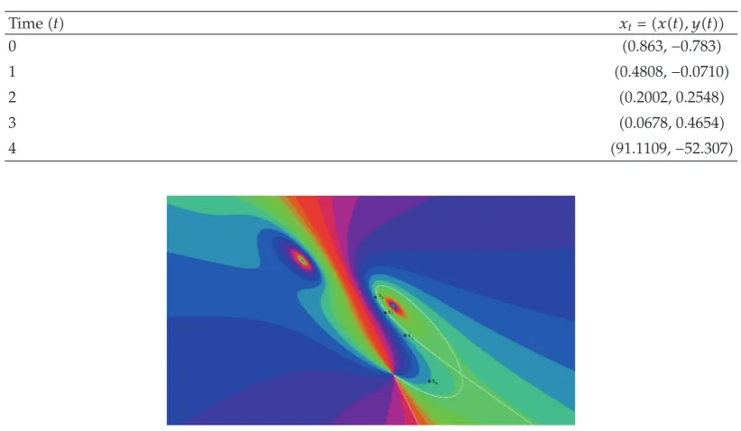
Table 1: Coordinates of the intersection of the level curveshx, y −1.68195 andh2x, y 2.26841−tfor

t0,1,2,3,4.

Timet xt xt, yt

0 0.863,−0.783

1 0.4808,−0.0710

2 0.2002, 0.2548

3 0.0678, 0.4654

4 91.1109,−52.307

Figure 1: Visualization of the trajectories of5.26. In this case we have plotted level bands ofhx, y, so that

the trajectories are in fact the boundaries between the colored bands. We have also plotted, in white, the trajectory that passes through a singular point corresponding to a pole of thecomplexanalytic function

gz. To exemplify the parametrization, we have plotted in black the points corresponding tot0,1,2,3

see Table1.

In order to parametrize the solution we need to calculateh2x, ywhich turns out to

be

h2

x, y −arctan

₋₁ _x ₂_y

1−2x−y

arctan

₁₋_x₋₂_y

1 2x y

−1

2log

2x y2 1 x 2y2.

5.27

According to Corollary 5.8 we proceeded to calculate the intersection the level curves

hx, y −1.68195 and h2x, y 2.26841−t fort 0,1,2,3,4. The results are shown in

Table1and as black dots in Figure1.

Acknowledgments

[image:19.600.209.401.467.557.2]

(20)

References

1 L. Bers, Theory of Pseudo-Analytic Functions, Institute for Mathematics and Mechanics, New York University, New York, NY, USA, 1953.

2 L. Bers, “An outline of the theory of pseudoanalytic functions,” Bulletin of the American Mathematical

Society, vol. 62, pp. 291–331, 1956.

3 M. D ¨uz and K. Koca, “A Dirichlet problem for generalized analytic functions,” Selc¸uk Journal of Applied

Mathematics, vol. 7, no. 1, pp. 9–15, 2006.

4 S. B. Klimentov, “BMO classes of generalized analytic functions,” Vladikavkazski˘ı Matematicheski˘ı

Zhurnal, vol. 8, no. 1, pp. 27–39, 2006.

5 V. Kravchenko, “On the relationship between p-analytic functions and Schr ¨odinger equation,”

Zeitschrift f ¨ur Analysis und ihre Anwendungen, vol. 24, no. 3, pp. 487–496, 2005.

6 A. Meziani, “Elliptic planar vector fields with degeneracies,” Transactions of the American Mathematical

Society, vol. 357, no. 10, pp. 4225–4248, 2005.

7 Le Thu Hoai and W. Tutschke, “Associated spaces defined by ordinary diﬀerential equations,”

Zeitschrift f ¨ur Analysis und ihre Anwendungen, vol. 25, no. 3, pp. 385–392, 2006.

8 W. Tutschke, “Interactions between partial diﬀerential equations and generalized analytic functions,”

Cubo, vol. 6, no. 1, pp. 281–292, 2004.

9 W. Tutschke, “Generalized analytic functions in higher dimensions,” Georgian Mathematical Journal, vol. 14, no. 3, pp. 581–595, 2007.

10 I. N. Vekua, Generalized analytic functions, Pergamon Press, Addison-Wesley, London, UK, 1962.

11 Z.-l. Xu, “Mixed elastico-plasticity problems with partially unknown boundaries,” Acta Mathematicae

Applicatae Sinica (English Series), vol. 23, no. 4, pp. 629–636, 2007.

12 M. Zabarankin and P. Krokhmal, “Generalized analytic functions in 3D Stokes flows,” The Quarterly

Journal of Mechanics and Applied Mathematics, vol. 60, no. 2, pp. 99–123, 2007.

13 M. Zabarankin, “The framework of k-harmonically analytic functions for three-dimensional Stokes flow problems. I,” SIAM Journal on Applied Mathematics, vol. 69, no. 3, pp. 845–880, 2008.

14 B. Ziemian, “Generalized analytic functions with applications to singular ordinary and partial diﬀerential equations,” Dissertationes Mathematicae (Rozprawy Matematyczne), vol. 354, 100 pages, 1996.

15 K. Hockett and S. Ramamurti, “Dynamics near the essential singularity of a class of entire vector fields,” Transactions of the American Mathematical Society, vol. 345, no. 2, pp. 693–703, 1994.

16 T. Newton and T. Lofaro, “On using flows to visualize functions of a complex variable,” Mathematics

Magazine, vol. 69, no. 1, pp. 28–34, 1996.

17 A. Garijo, A. Gasull, and X. Jarque, “Local and global phase portrait of equation ˙zfz,” Discrete

and Continuous Dynamical Systems A, vol. 17, no. 2, pp. 309–329, 2007.

18 A. Alvarez-Parrilla, A. G ´omez-Arciga, and A. Riesgo-Tirado, “Newton vector fields on the plane and on the torus,” Complex Variables and Elliptic Equations, vol. 54, no. 5, pp. 440–461, 2009.

19 A. Alvarez-Parrilla, J. Mucino-Raymundo, S. Solorza-Calderon, and C. Yee-Romero, Complex Analytic

Vector Fields: Geometry, Dynamics and Visualization, 2009.

20 H. E. Benzinger, “Julia sets and diﬀerential equations,” Proceedings of the American Mathematical Society, vol. 117, no. 4, pp. 939–946, 1993.

21 F. von Haeseler and H. Kriete, “The relaxed Newton’s method for rational functions,” Random and

Computational Dynamics, vol. 3, no. 1-2, pp. 71–92, 1995.

22 F. von Haeseler and H. O. Peitgen, “Newton’s method and complex dynamical systems,” Acta

Applicandae Mathematicae, vol. 13, no. 1-2, pp. 3–58, 1988.

23 S. Smale, “A convergent process of price adjustment and global Newton methods,” Journal of

Mathematical Economics, vol. 3, no. 2, pp. 107–120, 1976.

24 E. Kreyszig, Introductory Functional Analysis with Applications, John Wiley & Sons, 1978.

25 W. C. Brown, Matrices Over Commutative Rings, Marcel Dekker, New York, NY, USA, 1993.

26 E. R. Lorch, “The theory of analytic functions in normed Abelian vector rings,” Transactions of the

American Mathematical Society, vol. 54, pp. 414–425, 1943.

27 J. A. Ward, “From generalized Cauchy-Riemann equations to linear algebras,” Proceedings of the

American Mathematical Society, vol. 4, no. 3, pp. 456–461, 1953.

28 R. D. Wagner, “The generalized Laplace equations in a function theory for commutative algebras,”

Duke Mathematical Journal, vol. 15, pp. 455–461, 1948.

29 P. W. Ketchum, “Analytic functions of hypercomplex variables,” Transactions of the American

Mathematical Society, vol. 30, no. 4, pp. 641–667, 1928.

(21)

31 L. V. Ahlfors, Complex Analysis, An Introduction to the Theory of Analytic Functions of One Complex

Variable, McGraw-Hill, New York, NY, USA, 3rd edition, 1979.

32 R. E. Greene and S. G. Krantz, Function Theory of One Complex Variable, vol. 40 of Graduate Studies in

Mathematics, American Mathematical Society, Providence, RI, USA, 2nd edition, 2002.

(22)

Submit your manuscripts at

http://www.hindawi.com

Hindawi Publishing Corporation

http://www.hindawi.com Volume 2014

Mathematics

Journal of

http://www.hindawi.com Volume 2014 in Engineering

Hindawi Publishing Corporation http://www.hindawi.com

Differential Equations

International Journal of

Volume 2014

Applied MathematicsJournal of

Probability and Statistics Hindawi Publishing Corporation

Journal of

http://www.hindawi.com Volume 2014 Mathematical PhysicsAdvances in

Complex Analysis

Journal of Hindawi Publishing Corporation

Optimization

Journal of

Combinatorics

http://www.hindawi.com Volume 2014 International Journal of

Operations Research

Journal of

Function Spaces

Abstract and Applied Analysis

International Journal of Mathematics and Mathematical Sciences

Hindawi Publishing Corporation http://www.hindawi.com Volume 2014

The Scientific

World Journal

Algebra

Discrete Dynamics in Nature and Society Hindawi Publishing Corporation

Decision Sciences

Discrete Mathematics

Journal of

On Solving Systems of Autonomous Ordinary Differential Equations by Reduction to a Variable of an Algebra

Research Article